

- EAER>
- Journal Archive>
- Contents>
- articleView
Contents
Citation
| No | Title |
|---|
Article View
East Asian Economic Review Vol. 22, No. 3, 2018. pp. 337-370.
DOI https://dx.doi.org/10.11644/KIEP.EAER.2018.22.3.347
Number of citation : 0View
68
Download
70
Exchange Rate Pass-through, Nominal Wage Rigidities, and Monetary Policy in a Small Open Economy
|
|
Department of Economics, University of Windsor |
|---|---|
|
|
School of Economics, Chung-Ang University |

Abstract
This paper discusses the design of monetary policy in a New Keynesian small open economy framework by introducing nominal wage rigidities and incomplete exchange rate pass-through on import prices. Three main findings are summarized. First, with the existence of an incomplete exchange rate pass-through and nominal wage rigidities, the optimal policy is to seek to minimize the output gap, the variance of domestic price and wage inflation, as well as deviations from the law of one price. Second, the CPI inflation targeting Taylor rule is welfare enhancing when there is a technological shock to the economy. The exception occurs when there is a foreign income shock, which minimizes welfare losses under the domestic inflation targeting Taylor rule. Last, two stylized Taylor rules turn out to be a bad approximation, but the modified Taylor rules that respond to the unemployment gap rather than the output gap are a closer approximation to the optimal policy.
JEL Classification: E31, E58, F4
Keywords
Incomplete Pass-through, Nominal Wage Rigidities, Modified Taylor Rule, Monetary Policy, Small Open Economy
I. INTRODUCTION
Recent effort devoted to developing dynamic stochastic general equilibrium models of open economies, so-called New Open Economy Macroeconomics (NOEM henceforth), use highly stylized models to determine welfare under alternative exchange rate regimes to derive optimal monetary policy rules (e.g., McCallum and Nelson, 2000; Clarida et al., 2002; Benigno and Benigno, 2003; Galí and Monacelli, 2005). These studies have led to the well-known traditional recommendation to monetary policy makers in open economies: optimal monetary policy in an open economy requires exchange rate flexibility and domestic inflation stabilization. A common assumption in this literature is that the law of one price continually holds; therefore the pass-through of the exchange rate to import prices is complete. However, the empirical evidence suggests that changes in the exchange rate do not tend to ‘pass-through’ quickly to the price of import goods. Therefore, the price of traded goods and consumer prices are almost unresponsive to changes in the exchange rate (See Rogoff, 1996; Goldberg and Knetter, 1997; Obstfeld and Rogoff, 2000).
As a result, numerous NOEM researchers have been motivated to construct a realistic representation of an incomplete pass-through of exchange rates. This type of NOEM research characterizes local currency pricing and studies the impact of an incomplete pass-through on the optimal conduct of monetary policy and related issues in open economies (e.g., Devereux and Engel, 2003; Corsetti and Pesenti, 2005; Monacelli, 2005; Sutherland, 2005; Takhtamanova, 2010; Daniels and VanHoose, 2013; Donayre and Panovska, 2016). In contrast to the former NOEM literature, this research finds that when there is incomplete pass-through of exchange rates, the stabilizing role of flexible exchange rates may not be as strong and welfare maximizing monetary policy requires stabilization of the CPI inflation. Another issue addressed in this research concerns the relative usefulness of an exchange rate target for the conduct of monetary policy (e.g., Batini et al., 2001; Kollmann, 2002; Smets and Wouters, 2002; Leitemo and Söderström, 2005; Adolfson, 2007). This literature has explored a broad set of exchange rate augmented policy rules, without attaining complete consensus of whether or not it is beneficial to include some feedback from an exchange rate variable in the central bank’s instrument rule.
A significant limitation shared by all these studies is that the models tend to ignore the importance of the labor market frictions (wage rigidities and unemployment fluctuations) and assign labor markets a secondary role. However, many authors have noted that labor market behavior is key to understating the adjustment process in small open economies. Over the past few years, a number of researchers have incorporated labor market frictions and unemployment into the closed economy dynamic stochastic general equilibrium model (e.g., Blanchard and Galí, 2010; Galí, 2011; Ravenna and Walsh, 2011; Thomas, 2008). Surprisingly, much less attention has been devoted to the open economy counterpart of such a paradigm. The recent works by Campolmi (2014), and Campolmi and Faia (2015) are among notable exceptions.
This paper departs from the previous NOEM literature by introducing some frictions in the labor market (nominal wage rigidities and unemployment) and analyzing their consequences for monetary policy. The introduction of monopoly power of labor supply and resulting wage rigidities is motivated by some stylized facts in labor dynamics in many European countries. It has been observed that Europe is characterized by more unionized and by a high degree of wage rigidity than the U.S, which leads to very slow adjustment of Europe’s labor markets (Dickens et al., 2007). As a result, all variations in labor input take place in the form of variations in employment. Since this study builds on Galí and Monacelli (2005) and Monacelli (2005), it is worth clarifying the points at which this paper departs from this work. The structure of the model in this article differs in three respects. First, the model allows nominal wage rigidities. This is done by assuming that each household with monopoly power in the labor market sets the nominal wages in a staggered contract with timing like that of Calvo (1983). Then, combined with incomplete pass-through of exchange rates on import prices, the sluggish adjustment of nominal wages generates a more muted response of real wage. Second, based on the work of Galí (2011), we modify the labor market and introduce unemployment into the small open economy model. In this framework, we find that changes in terms of trade and the exchange rate have a direct effect on the equilibrium level of employment in a small open economy. We also find that unemployment and its fluctuations are affected by the degree of pass-through of exchange rates. By introducing unemployment into the standard NOEM model, this paper is able to address issues regarding unemployment fluctuations in open economies and study some of the normative implications of the existence of unemployment due to sticky nominal wages for the conduct of monetary policy. As pointed out below, the model with unemployment fluctuation has different implications for the design of alternative simple policy rules. Especially, the introduction of unemployment in the model allows us to study the properties of a simple interest rate rule that has unemployment as an argument. Third, we derive a second-order approximation of the average welfare losses experienced by representative households under incomplete pass-through of exchange rates and nominal wage rigidities. Galí and Monacelli (2005) derive welfare function under the complete pass through, and Monacelli (2005) assumes a quadratic loss function which penalizes the variability of CPI inflation and output gap around some target values. The model developed in this paper focuses on the effects of two sources of exogenous disturbances; country-specific shocks (domestic technology shocks) and shocks originated from abroad (foreign income shocks).
The paper argues that the combination of an incomplete pass-through of exchange rates and nominal wage rigidities yield important implications for the design of monetary. First, we show that an explicit derivation of welfare function can be expressed in terms of the unconditional variances of the output gap, domestic price, wage inflation, and the law of one-price gap. In this model, the welfare losses include another source of welfare losses, associated with fluctuations of wage inflation and the law of one price gaps. The presence of sticky wages and the deviations from the law of one price leads to the utility losses experienced by the representative consumer as a consequence of deviations from the efficient allocation. As a result, the optimal policy seeks to minimize a weighted average of these variances.
Second, the optimal inflation target for simple policy rules may be CPI inflation or domestic price inflation depending on the source of the exogenous disturbance. We find that the CPI inflation targeting rule produces relatively small welfare losses incurred by a domestic technology shock. The CPI inflation targeting rule, however, also generates the excess smoothness of both the terms of trade and the nominal exchange rate to a foreign income shock. Thus, the stabilizing power of the CPI inflation targeting rule is diminished, as it hinders adjustment that might have occurred through exchange rate movement.
Third, two-stylized Taylor rules (CPI and domestic inflation targeting rules) turn out to be a bad approximation to the optimal policy. However, the modified Taylor rules that respond to the unemployment gap rather than output gap are welfare enhancing and are a closer approximation to the optimal policy. This result does not depend on types of shocks and types of inflation targets. This result has important implication for the monetary policy design in practice: The interest rate rule requires that the domestic interest rate responds systematically to unemployment rate rather than output gap works well regardless of types of shocks and types of inflation targets. Galí (2011) argues that such a rule provides a good account of the Fed’s interest rate decisions during 1987 to 2008 period.
The plan of this paper is as follows. We present the basic model in section II, while section III describes the equilibrium conditions and the dynamic system of the model. In section IV, the relationship between dynamic responses of the model and the degree of pass-through of exchange rates on local import prices is examined. The implications and performance of optimal and alternative monetary policy regimes are discussed in section V. In section VI, we draw the main conclusions.
II. MODEL
1. Households
The home country is populated by a large number of identical households. Each household has a continuum of members represented by the unit square and indexed by a pair (

where
The household’s period utility is given by the integral of its member’s period utilities and can be written as

where 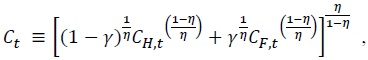 with
with 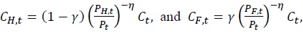 where
where 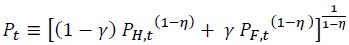 is the consumer price index (CPI) with the domestic price index (
We assume that households have access to a complete set of state-contingent securities traded internationally. Under the assumption of full consumption risk sharing across households, the household’s intertemporal optimality condition is standard and can be written as

where lower case letters denote the log-deviations of the respective variables from their steady states, ρ ≡ −log
(1) Optimal Wage Setting
Following Erceg, Henderson, and Levin (2000), we assume that each household supplies a differentiated labor service indexed. Furthermore, each household (with monopoly power in the labor market) sets nominal wages in a staggered fashion with timing as in Calvo (1983): in each period, only a fraction (1 −

where  denotes the (log) of the newly set nominal wage,
  which corresponds to the log of the optimal or desired wage mark-up.
Let denote  the deviation of the economy’s (log) average wage markup as

where 
(2) Unemployment
Next, we introduce unemployment and discuss its relation with the wage markup. As shown in Galí (2011), the log approximation of the aggregate labor supply or participation condition is given by

where  are the first-order approximation of aggregate labor force or participation around its symmetric steady state.
We define the unemployment rate,

Then, using the definition of the average wage mark-up, we can obtain the following simple relation between the wage markup and the unemployment rate:

Equation (6) shows that unemployment fluctuation is a consequence of variations in the wage markup, which are the result of nominal wage rigidities.
(3) Foreign Country
To keep the analysis simple, we assume that there are two countries, home ( The optimal allocation of expenditures for domestic goods is given by
2. Domestic Goods Producers
Next, we consider the production side of the economy. The market for domestic goods in the home country is populated by a continuum of domestic firms acting as monopolistic competitors indexed by z∈[0,1], whose total is normalized to unity. Each domestic firm produces a differentiated good with a technology represented by the production function (in the log-linear term)  and
and
Given the wages at any point in time, cost minimization yields the following real marginal cost in terms of domestic goods prices (in log term)

where
We now turn to the pricing decisions of domestic firms. Following Calvo (1983), we assume that a fraction of 1 −

where  denotes the log of newly set domestic prices, and
  which corresponds to the log of the optimal price mark-up in a flexible price equilibrium or in the steady state. Then, the (log-linearized) optimal price-setting condition (8) can be combined with the (log-linearized) difference equation describing the evolution of domestic prices to yield an equation determining domestic inflation as a function of deviations of marginal cost from its steady state value

where 
3. Importer
In this section, we present the model that considers the incomplete pass-through of exchange rates on imported goods prices. Following Monacelli (2005), we assume that there are many domestic retailers who import differentiated foreign goods. The law of one price holds at the wholesale import stage, but the domestic currency prices of these goods deviate from the foreign prices at the consumer stage.
Consider the pricing decision of domestic retailers importing foreign good  that maximizes

subject to the sequence of demand constraints

where  is the marginal cost of importing (domestic currency price paid in the foreign market),
 is the foreign currency price of the imported good, and Λ
As shown in Monacelli (2005), the optimal price-setting strategy in period t can be approximated by the (log-linear) rule

where  denotes the (log) of the newly set domestic currency price of imported goods,
  which corresponds to the log of the optimal price mark-up in a flexible price equilibrium or in the steady state, and

where
Following Monacelli (2005), we define this deviation as the law of one price gap (l.o.p gap henceforth). The l.o.p gap ( The log-linear aggregate import price evolves according to

By combining equations (10) and (12), we obtain the Phillips curve for imported goods described by

where  Equation (13) implies that import price inflation rises as the l.o.p gap increases. The rise in the l.o.p gap acts as an increase in real marginal cost and therefore boosts foreign goods inflation.
III. EQUILIBRIUM
1. Aggregate Demand
Goods market clearing in the home country requires  for all good
  yields a following log-linear approximation of aggregate demand around the steady state is:

where 
The log-linear approximation of the international risk sharing condition, recognizing that

where,
Finally, combining equation (14) with the Euler equation (1), we obtain the dynamic IS equation for the small open economy:

where  denotes the output gap, and

is the small open economy’s natural rate of interest. Thus, aggregate demand is characterized by a forward-looking IS equation similar to that found in the standard open economy model. There is a major difference however, that must be pointed out. The current output gap depends on the expected future changes in the l.o.p gap to the extent that
2. Supply Side
We introduce the real wage gap as the deviation of current real wage from its natural level,

Using the fact that  we relate the average price markup to the output, real wage, and l.o.p gaps

Hence, combining equations (9) and (18) yields

where  Equation (19) represents the equation for domestic price inflation. From equation (19), we see that movement in domestic inflation can result from endogenous movements in the l.o.p gap. The sign of the relationship between the l.o.p gap and domestic inflation is negative. This finding contrasts with Monacelli (2005), where the movements of domestic inflation and the l.o.p gap were positively related. In Monacelli (2005), a change in l.o.p gap has an effect on the domestic inflation through its impact on real wage and the terms of trade. Since the nominal wages are flexible the rise in l.o.p gap, ends up increasing real wage through the wealth effect on labor supply, resulting from its impact on consumption. However, the result in equation (15) implies that for a given output positive change in the l.o.p gap has a negative effect on terms of trade. Thus the rise in the l.o.p gap reduces the real marginal cost through the terms of trade effect. In Monacelli (2005), however, the wealth effect dominates terms of trade effect. Thus, the movements of domestic inflation and the l.o.p gap were positively related. In the preset model, there is no wealth effect due to nominal wage rigidities. Hence (for any given output gap) positive movements in domestic inflation can result from negative movements in the terms of trade which can in turn be induced by positive variations in the l.o.p gap.
Similarly, relating the average wage markup to the output and real wage gaps yields

Therefore, we can derive the following equation for wage inflation

where  Unlike domestic price inflation, the positive movement in wage inflation can result from a positive movement in the l.o.p gap. Through its impact on consumption, a rise in the l.o.p gap will reduce the wage mark-up. Therefore, wage inflation rises as the l.o.p gap increases.
Combining equations (6) and (20) leads to the following equation describing the relationship between the unemployment, output, real wage, and the l.o.p gaps as

Since a positive movement in the l.o.p gap increases the wage markup, the unemployment gap is negatively related to the l.o.p gap.
Finally, in order to close the model, we specify how the interest rate is determined. This is done by assuming a Taylor-type interest rule of the form

where π
The effect of adding the incomplete pass-through results in a modification of the recent New Keynesian open economy aggregate demand and supply relationships. In Monacelli (2005), the introduction of incomplete pass-through has the effect of appending the deviations from the law of one price as positive supply shocks to domestic inflation. By inspecting domestic inflation equation (19) and wage inflation equation (21), we can see that combined with nominal wage rigidities, the deviations from the law of one price acts as a negative shock to domestic inflation, but a positive shock to wage inflation. Therefore, the contrasting behavior of domestic inflation and wage inflation in response to the deviations from the law of one price will be critical to understand the equilibrium dynamics and monetary policy design problem of the model.
IV. MONETARY POLICY DESIGN
This section explores the implications of the existence of an incomplete passthrough of exchange rates on local import prices and nominal wage rigidities in a small open economy, as modeled in section 2, for the conduct of monetary policy. We assume that the domestic government chooses a subsidy rate that makes the natural level of output corresponding to the efficient level in a zero inflation steady state. It is also assumed that the efficiency of the flexible price equilibrium allocation holds throughout this study.
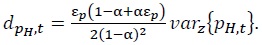
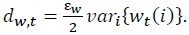
As we show in the appendix, to derive the central bank’s objective function, we take the second-order approximation of the utility of the representative household around the zero-inflation steady state, under the assumption of η = 1. After an appropriate normalization, we obtain the following quadratic objective, where the welfare loss from a deviation from the optimum is expressed as a fraction of the steady-state consumption, given by

where  and
and

Note that the relative weight of each of the variances is a function of the underlying parameter values. The period welfare loss (25), is similar to that derived in Campolmi (2014) except for its dependence on the l.o.p gap. In this model, the welfare losses include another source of welfare losses, associated with the law of one price gaps. The presence of the deviations from the law of one price leads to the utility losses experienced by the representative consumer as a consequence of deviations from the efficient allocation. Corsetti and Pesenti (2001), Monacelli (2005), Benigno and Benigno (2006), De Paoli (2009) and others argue that the exchange rate term should appear in the loss function due to the fact that, in general, and under a number of different circumstances, movement in the real exchange rate has an effect on welfare. In this study, we are able to consider the welfare effects of the exchange rate movement through the l.o.p gap in the loss function (25).
We are now ready to characterize optimal policy for our small open economy. The central bank will seek to minimize (24) subject to the sequence of equilibrium constraints given by (11), (13), (19), and (21). Due to the presence of deviation of the law of one price and dependence of welfare function on it, optimal policy should stabilize the fluctuations of the law of one price gap as well as other sources of welfare losses including wage inflation.
1. Calibration
This section computes numerically the dynamic response of the model to different types of shocks for a calibrated version of the small open economy developed in the previous section. Specifically, we focus on how the presence of an incomplete pass-through of exchange rates together with nominal wage rigidities influence the economy’s response to the shocks. The setting chosen for many of the parameters is from Galí and Monacelli (2016) that is reasonable with the evidence for euroarea countries like Greece, Italy, Portugal, and Spain over the 1999-2014 period (see, e.g., Christoffel, Coenen, and Warne, 2008). In the baseline calibration of the model, one period corresponds to one quarter of a year. We assume Therefore, we set

where  are white noises with variances
2. Evaluation of Alternative Monetary Policy Rules
This section considers several simple monetary policy rules and presents some quantitative evaluations based on a calibrated version of a small open economy under the existence of an incomplete pass-through of exchange rates on the local import price. The evaluation is based on the unconditional variances of major variables and associated welfare losses given the baseline calibration. Four different simple policy rules are studied. The general specification of monetary policy rules take a form of

where
• Rule 1: CPI inflation targeting with output gap (
• Rule 2: Domestic inflation targeting with output gap (
• Rule 3: CPI inflation targeting with unemployment gap (
• Rule 4: Domestic inflation targeting with unemployment gap (
Figure 1 displays the dynamic responses of the main macro variables considered in the previous section, to an exogenous domestic productivity shock under different policy rules. For the sake of comparison, we also display the responses under the optimal rule. We start by describing impulse responses under the optimal policy. Not surprisingly, we see that the major variables (domestic price, wage inflation and the output gap), remain stable to the shock under the optimal policy. It is also seen that the optimal policy leads to a more stable response from the unemployment gap. This implies that the optimal policy is more accommodative towards a technological shock than any other alternative policies. The optimal policy reaction leads to a reduction in the domestic interest rate, as is needed to support the expansion in consumption and output consistent with the natural rate equilibrium. Given the constancy of the foreign interest rate, uncovered interest parity implies an initial nominal depreciation followed by an expected appreciation. Thus, under the optimal rule, there is an initial increase in the l.o.p gap, reverting gradually to the steady state afterward. The rise in the l.o.p gap leads to an increase in the import price inflation (not shown in figure 1). The responses of the domestic price and wage inflation are also muted. However, the response of the CPI inflation, mirrored by the response of the import price inflation, is considerably volatile.
The same figure displays the corresponding impulse responses under different simple policy rules. The responses of the main variables are almost identical under different policies. Notice that simple policy rules generate more volatile responses of key variables than the optimal policy except l.o.p gap, which shows a more muted response under simple policy rules. Both CPI and domestic inflation, mirrored by the muted response from the l.o.p gap, are also much less volatile. Notice that the performance of simple policy rules is different from optimal policy not only qualitatively, but also qualitatively. This is due to the fact that unlike simple policy rules, optimal policy, by responding to changes in the l.o.p gap, can minimize any induced fluctuations in domestic inflation and the output gap. The optimal policy also explicitly stabilizes wage inflation, which generates more muted responses of domestic inflation and the output gap.
The left panel of Table 1 contrasts the statistical properties of some key variables generated under different simple policy rules with those implied by the optimal policy, conditional on a technology shock. The main finding is that the CPI inflation targeting rule is relatively more accommodative of the productivity shock than domestic inflation policy rules, with the l.o.p gap remaining relatively stable. Therefore, the responses of the key variables are relatively more muted under the CPI inflation targeting rule than domestic inflation targeting. It is also shown that monetary policies in which interest rate responds to unemployment gap rather than the output gap generate more muted responses of key variables.
Figure 2 shows the responses of the same variables to a foreign income shock under the optimal policy and alternative policy rules. The relevant second moments conditional on the foreign income shock are also shown in the right panel of Table 1. As would be expected, the optimal policy stabilizes the major variables (domestic price, wage inflation and the output gap), by fully accommodating the foreign income shock. The responses of the same variables are similar under alternative policy rules. There exists notable difference, however, in that the domestic inflation targeting rule generates a more muted response from the key variables. The critical feature that distinguishes the impact of a technological shock on an economy’s dynamic responses relative to a foreign income shock is the excess volatility of the terms of trade and the nominal exchange rate. Thus, the response of the CPI inflation is more volatile with a technological shock. Therefore, the CPI inflation targeting rule leads to smoothness of the terms of trade and the nominal exchange rate. This, in turn, is reflected by a muted response from the real wage. The controlling of CPI inflation reduces unemployment fluctuation by stabilizing the real wage.
In Figure 2, the responses of the terms of trade and the nominal exchange rate to a foreign income shock are relatively more muted. Thus, the stabilization of CPI inflation is partly achieved by less volatile movements in the nominal exchange rate with a foreign income shock. The CPI inflation targeting rule generates the excess smoothness of both the terms of trade and the nominal exchange rate with a foreign income shock. Thus, it hinders adjustment that might have occurred through exchange rate movement which causes the stabilizing power of the CPI inflation targeting rule to be diminished. The policies that respond to unemployment gap rather than output gap also generate more muted responses of key variables to a foreign income shock.
Table 2 reports the variances of the domestic price, wage inflation, output, and the l.o.p, as well as the welfare losses associated with four different simple policy rules. In addition to the simple rules, the table also reports the corresponding statistics for the optimal policy, which provides a useful benchmark. We display the effects of changing the inverse of the Frisch elasticity of labor supply (as implied by changes in φ). The top panel reports statistics corresponding to the benchmark calibration of the elasticity of labor supply, namely, φ = 5. Relative to that benchmark, the second panel assumes a lower inverse of the Frisch elasticity of labor supply (φ = 1), while the third-panel reports result for a higher inverse of the Frisch elasticity of labor supply (φ = 10). The main findings of this exercise are consistent with the quantitative evaluation conducted in Table 2. Under all of the calibrations considered, conditional on the technology shock, the CPI inflation targeting rule generates relatively small welfare losses. However, the welfare losses are minimized under the domestic inflation targeting rule when there is a foreign income shock. Regardless of types of shocks and inflation targets, monetary policies stabilizing unemployment gap rather than the output gap generate relatively small welfare losses.
In this exercise, it is shown that the performance of simple policy rules fails to approximate that of optimal policy if both an incomplete pass-through of the exchange rate and nominal wage rigidities exist. The responses of key variables, especially l.o.p gap, unemployment gap, and wage inflation under the optimal policy are more muted than those of two frequently-used Taylor rules (CPI and domestic inflation targeting rules), not only qualitatively, but also qualitatively. This is because the optimal policy responds to fluctuations of the l.o.p gap and nominal wage inflation, but two-stylized Taylor rules (CPI and domestic inflation targeting rules do not respond to these fluctuations. By responding to the movements of the l.o.p gap and the nominal wage inflation, the optimal policy can also reduce any induced fluctuations in the unemployment gap. It can be seen from equation (22).
This study also shows that the modified two Taylor rules in which interest rate responds to unemployment gap rather than the output gap generate more muted responses of key variables and smaller welfare losses. By reducing fluctuations in unemployment gap, it can indirectly stabilize the l.o.p gap, output gap, and the real wage gap. The response of nominal wage inflation is also reduced when the real wage gap is stabilized. Therefore, it can be argued that alternative policy rules where the interest rate responds to the unemployment gap, as well as inflation rate, could be a closer approximation to the optimal policy. This is due to the fact that the unemployment gap is related to real wage, output and the law of once price gap.
By stabilizing the unemployment gap, the central bank is able to reduce fluctuations of the wage gap, output gap and the law of once price gap.
The above results have another implication for exchange rate policy. If the central bank explicitly targets exchange rate stabilization, it should adopt CPI inflation targeting rather than domestic inflation targeting. Now CPI inflation can be expressed in terms of the exchange rate as

As it can be seen from the above equation, by controlling the volatile movements of CPI inflation, the central bank can reduce exchange rate fluctuations.”
V. CONCLUSION
In this paper, we incorporate both an incomplete exchange rate pass-through on import prices and nominal wage stickiness into a standard New Keynesian small open economy model of Galí and Monacelli (2005) and study its implications for monetary policy. Within this framework, we study the optimal monetary policy rule and compare the performances of alternative policy rules. In order to do that we derive a second-order approximation of the average welfare losses, which turns out to be quite different from that of Galí and Monacelli (2005) and Campolmi (2014). The main findings for this part of the study can be summarized as follows. First, the optimal policy is to seek to minimize the variances of the domestic price, wage inflation, the output gap, and the law of one price gap. Obviously, this result is different from Galí and Monacelli (2005), where the optimal policy minimizes the variances of the domestic price and the output gap only, and also from Campolmi (2014) in which the variances of the wage inflation, in addition to the variances of domestic inflation and output gap, is minimized. Second, the CPI inflation targeting rule is welfare enhancing when there is a technological shock. However, the welfare losses are minimized under the domestic inflation targeting rule if there is a foreign income shock. This result is also in sharp contrast with the previous result. Galí and Monacelli (2005) argue that domestic inflation targeting produces minimum welfare losses, but, Monacelli (2005) argues for CPI inflation targeting under the incomplete exchange rate pass-through. This paper also finds that the two stylized Taylor rules (CPI and domestic inflation targeting rules) turn out to be a bad approximation to the optimal policy, but the stabilizing unemployment gap rather than output gap in stylized Taylor-rules is welfare enhancing regardless of types of shocks and inflation targets.
Our study has some obvious limitations that may indicate possible directions for future work. First, as pointed out by Galí (2011), the only source of unemployment is the positive wage markup from the noncompetitive labor market. However, as shown in the text, the wage markup is easily fixed by simple fiscal policy (an employment subsidy). Therefore, introducing certain forms of real frictions into the labor market would improve the model’s performance. One way is by introducing matching frictions. This is, for example, the approach followed by Blanchard and Galí (2010), and Ravenna and Walsh (2011), in a closed economy model. Thus, it would be interesting to introduce unemployment by means of matching frictions, and then extend the work by Blanchard and Galí (2010) and Ravenna and Walsh (2011) to a small open economy. By doing so, the unemployment rate would enter directly into the welfare function and would thus play a critical role in the optimal monetary policy.
There are a number of papers that incorporate imported inputs of production into the context of a New Keynesian small open economy model in order to study monetary policy issues (e.g., McCallum and Nelson, 1999, 2000). Therefore, it would be interesting to include a role for imported inputs of production that allows for an incomplete passthrough of the exchange rate on the imported input price, and study how this extension affects the major findings in the paper.
Tables & Figures
Figure 1.
Impulse Responses to a Technological Shock: Alternative Policy Rules

Table 1.
Statistical Properties of Alternative Policy Regimes

Note: Standard deviations expressed in percent.
Rule 1: CPI inflation targeting with output gap (
Rule 2: Domestic inflation targeting with output gap (
Rule 3: CPI inflation targeting with the unemployment gap (
Rule 4: Domestic inflation targeting with the unemployment gap (
Figure 2.
Impulse Responses to a Foreign Income Shock: Alternative Policy Rules

Table 2.
Contribution to welfare losses

Table 2.
Continued

Note: Entries are percentage units of natural output
Rule 1: CPI inflation targeting with output gap (
Rule 2: Domestic inflation targeting with output gap (
Rule 3: CPI inflation targeting with the unemployment gap (
Rule 4: Domestic inflation targeting with the unemployment gap (
Appendix A. Household’s Problem
In this appendix A, we derive the household’s intertemporal optimality condition, (1). A typical household seeks to maximize

subject to a sequence of budget constraints

where

is the consumer price index (CPI) with the domestic price index (

We assume that the household has access to a complete set of contingent claims traded internationally. The riskless short-term nominal interest rate,

The solution to the household’s intratemporal optimization problem yields the optimal demand for each good

The optimal allocation of expenditures between domestic and imported goods is also given by

Then the household’s intertemporal optimality condition is given by

Equation (A.1) is a standard Euler equation for intertemporal consumption decision and represents the expectational IS curve. Taking conditional expectations of both sides of the (A.1) and rearranging with the riskless short-term nominal interest rate, we obtain a standard stochastic Euler equation

Now, we write the standard stochastic Euler equation in log-linearized form as:

Appendix B. Optimal Wage Setting
Consider a household resetting its nominal wage in period  denote the newly set wage. Under the assumption of full consumption risk sharing across households, all households resetting their wage in any given period will choose the same wage. The household will choose in order to maximize

where remains in place.,


for

where  denotes the marginal rate of substitution between consumption and labor supply in period

where  which corresponds to the log of the optimal or desired wage mark-up.
Let us define the economy’s average marginal rate of substitution as  is the aggregate employment rate. Then, the (log) marginal rate of substitution in period

where the last equality makes use of (A.3). Hence, we can rewrite (A.5) as

Appendix C
In this appendix we derive a second-order approximation to the utility of the representative household around an efficient steady state. As has been discussed in the main text, we restrict our study to the special case of η = 1. Frequent use is made of the following fact:

where

where
Using the fact  and the market clearing condition
  and intergrating across households, we have

Define aggregate employment as 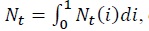 or, in terms of log deviations from the steady state and up to a second-order approximation,

Also, note that

where we have used the labor demand function 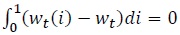 and that
 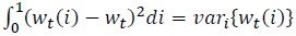 is of second order.
The next step is to derive a relationship between aggregate employment and output:

where 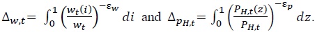 Thus, the following second-order approximation of the relation between (log) aggregate output and (log) aggregate employment holds:

where 
Proof. See Gali and Monacelli (2005).
Proof. See Erceg et al. (2000).
Now, one-period aggregate welfare can be written as


Proof. See Woodford (2003, Chapter 6).
Collecting the previous results, we can write the second-order approximation to the small open economy’s aggregate welfare function as follows:

where  and t.i.p. collects various terms that are independent of policy.
Appendix Tables & Figures
References
-
Adolfson, M. 2007. “Incomplete Exchange Rate Pass-through and Simple Monetary Policy Rules,”
Journal of International Money Finance , vol. 26, no. 3, pp. 468-494.
-
Batini, N., Harrison, R. and S. P. Millard. 2001. “Monetary Policy Rules for an Open Economy,”
Journal of Economics and Dynamic Control , vol. 27, no. 11, pp. 2059-2094. -
Benigno, G. and P. Benigno. 2003. “Price Stability in Open Economies,”
Review of Economic Studies , vol. 70, no. 4, pp. 743-764.
-
Benigno, G. and P. Benigno. 2006. “Designing Targeting Rules for International Monetary Policy Cooperation,”
Journal of Monetary Economics , vol. 53, no. 3, pp. 473-506.
-
Blanchard, O. and J. Galí. 2010. “Labor Markets and Monetary Policy: A New Keynesian Model with Unemployment,”
American Economic Journal: Macroeconomics , vol. 2, no. 2, pp. 1-30.
-
Calvo, G. 1983. “Staggered Prices in a Utility Maximizing Framework,”
Journal of Monetary Economics , vol. 12, no. 3, pp. 383-398.
-
Campolmi, A. 2014. “Which Inflation to Target?: A Small Open Economy with Sticky Wages,”
Macroeconomic Dynamics , vol. 18, no. 1, pp. 145-174.
-
Campolmi, A. and E. Faia. 2015. “Rethinking Optimal Exchange Regimes with Frictional Labour Market,”
Macroeconomic Dynamics , vol. 19, no. 5, pp. 1116-1147.
- Christoffel, K., Coenen, G. and A. Warne 2008. The New Area-Wide Model of the Euro Area-A Micro-Founded Open-Economy Model for Forecasting and Policy Analysis. European Central Bank Working Paper, no. 944.
-
Clarida, R., Galí, J. and M. Gertler. 2002. “A Simple Framework for International Monetary Policy Analysis,”
Journal of Monetary Economics , vol. 49, no. 5, pp. 879-904.
-
Corsetti, G. and P. Pesenti. 2001. “Welfare and Macroeconomic Interdependence,”
Quarterly Journal of Economics , vol. 116, no. 2, pp. 421-445.
-
Corsetti, G. and P. Pesenti. 2005. “International Dimensions of Optimal Monetary Policy,”
Journal of Monetary Economics , vol. 52, no. 2, pp. 281-305.
-
Daniels, J. P. and D. D. VanHoose. 2013. “Exchange-rate Pass Through, Openness, and the Sacrifice Ratio,”
Journal of International Money and Finance , vol. 36, 131-150.
-
De Paoli, B. 2009. “Monetary Policy and Welfare in a Small Economy,”
Journal of International Economics , vol. 77, no. 1, pp. 11-22.
-
Devereux, M. B. and C. Engel. 2003. “Monetary Policy in the Open Economy Revisited: Price Setting and Exchange Rate Flexibility,”
Review of Economic Studies , vol. 70, no. 4, pp. 765-783.
-
Dickens, W., Goette, L., Groshen, E., Holden, S., Messina, J., Schweitzer, M., Turunen, J. and E. Ward. 2007. “How Wages Change: Micro Evidence from the International Wage Flexibility Project,”
Journal of Economic Perspectives , vol. 21, no. 2, pp. 195-214.
-
Donayre, L. and I. Panovska. 2016. “State-dependent Exchange Rate Pass-through Behavior,”
Journal of International Money and Finance , vol. 64, pp. 170-195.
-
Erceg, C., Henderson, D. and A. Levin, 2000. “Optimal Monetary Policy with Staggered Wage and Price Contracts,”
Journal of Monetary Economics , vol. 46, no. 5, pp. 281-384.
-
Faia, E. 2008. “Optimal Monetary Policy Rules with Labor Market Frictions,”
Journal of Economics and Dynamic Control , vol. 32, no. 5, pp. 1600-1621.
-
Galí, J. 1999. “Technology, Employment, and the Business Cycle: Do Technology Shock Explain Aggregate?,”
American Economic Review , vol. 89, no. 1, pp. 249-271.
-
Galí, J. 2011.
Unemployment Fluctuations and Stabilization Policies: A New Keynesian Perspective . Cambridge: The MIT Press. -
Galí, J. and T. Monacelli. 2005. “Monetary Policy and Exchange Rate Volatility in a Small Open Economy,”
Review of Economic Studies , vol. 75, no. 3, pp. 707-734.
-
Galí, J. and T. Monacelli. 2016. “Understanding the Gains from Wage Flexibility: The Exchange Rate Connection,”
American Economic Review , vol. 106, no. 12, pp. 3829-3868.
-
Goldberg, P. and M. Knetter. 1997. “Goods Prices and Exchange Rates: What Have We Learned?,”
Journal of Economic Literature , vol. 35, no. 3, pp. 1243-1272. -
Kollmann, R. 2002. “Monetary Policy Rules in the Open Economy: Effects on Welfare and Business Cycles,”
Journal of Monetary Economics , vol. 49, no. 5, pp. 989-1015.
-
Leitemo, K. and U. Söderström. 2005. “Simple Monetary Policy Rules and Exchange Rate Uncertainty,”
Journal of International Money and Finance , vol. 24, no. 3, pp. 481-507.
-
McCallum, B. and E. Nelson. 1999. “Nominal Income Targeting in an Open-economy Optimizing Model,”
Journal of Monetary Economics , vol. 43, no. 3, pp. 553-578.
-
McCallum, B. and E. Nelson. 2000. “Monetary Policy for an Open-economy: An Alternative Framework with Optimizing Agents and Sticky Prices,”
Oxford Review of Economic Policy , vol. 16, no. 4, pp. 74-91.
-
Monacelli, T. 2005. “Monetary policy in a Low Pass-through Environment,”
Journal of Money and Credit Banking , vol. 36, no. 6, pp. 1047-1066.
-
Obstfeld, M. and K. Rogoff. 2000. “New Directions for Stochastic Open Economy Models,”
Journal of International Economics , vol. 50, no. 1, pp. 117-153.
-
Ravenna, F. and C. Walsh. 2011. “Welfare-based Optimal Monetary Policy with Unemployment and Sticky Prices: A Linear-quadratic Framework,”
American Economic Journal: Macroeconomics , vol. 3, no. 2, pp. 130-162.
-
Rogoff, K. 1996. “The Purchasing Power Parity Puzzle,”
Journal of Economic Literature , vol. 34, no. 2, pp. 647-668. -
Sutherland, A. 2005. “Incomplete Pass-through and the Welfare Effects of Exchange Rate Variability,”
Journal of International Economics , vol. 65, no. 2, pp. 375-399.
-
Smets, F. and R. Wouters. 2002. “Openness, Imperfect Exchange Rate Pass-through and Monetary Policy,”
Journal of Monetary Economics , vol. 49, no. 5, pp. 947-981.
-
Takhtamanova, Y. F. 2010. “Understanding Changes in Exchange Rate Pass-through,”
Journal of Macroeconomics , vol. 32, no. 4, pp. 1118-1130.
-
Taylor, J. 1993. “Discretion Versus Policy Rules in Practice,”
Carnegie-Rochester Series on Public Policy , vol. 39, pp. 195-214.
-
Thomas, C. 2008. “Search and Matching Frictions and Optimal Monetary Policy,”
Journal of Monetary Economics , vol. 55, no. 5, pp. 936-956.
-
Woodford, M. 2003. In
Interest and Price: Foundations of a Theory of Monetary Policy . Cambridge: MIT Press.