I. INTRODUCTION

Recent quantitative trade models based on the gravity equation have the attractive feature of being able to compute gains from trade using macro-level data and a small number of elasticities (see Arkolakis et al., 2012; Costinot and Rodriguez-Clare, 2014). A strength of this approach is that the gravity equation can been derived from diverse micro-theoretical foundations—the simple Armington set-up as in Anderson and van Wincoop (2003), perfect competition as in Eaton and Kortum (2002), Bertrand competition as in Bernard et al. (2003), monopolistic competition with homogeneous firms as in Krugman (1980), and models of monopolistic competition with firm-level heterogeneity à la Melitz (2003) as in Chaney (2008).1

Defining gains from trade as the absolute value of percentage change in real income associated with a movement to autarky from an observed equilibrium2 and using data for 2008 for 34 major economies, Costinot and Rodriguez-Clare (2014) show that gains from trade are in general greater for multiple sector models than single sector models, greater for models that allow for intermediate goods than models that do not, and greater for Melitz-style models than models that do not allow for firm heterogeneity. For the world as a whole, the gains from trade range from 4.4% for a one-sector model, to 14-15.3% for models with multiple sectors but without intermediates, to 27-40% for models with multiple sectors and intermediates.3

Utilizing the same framework and using the World Input-Output Database with 34 major countries (including a rest-of-the-world aggregate) and 31 sectors (including services), this paper analyzes changes in autarky gains from trade (i.e., welfare cost of autarky), as defined above, during the decade 1995-2006, a period of rapid globalization.4 It seeks to answer three questions: how autarky gains from trade have changed over time, what the proximate driving forces are, and what role trade costs have played in those changes. Changes are analyzed by comparing the start and end years of the decade under study—1995 and 2006.5 In a world that has of late been witnessing a backlash against globalization—most notably manifested in the ongoing US-China trade war—an analysis of gains from trade with respect to even as stark a counterfactual as autarky is helpful to put things in perspective.

There are three main findings. First, autarky gains from trade have increased during this period, by about 45% on average for the world, with heterogeneity across countries. Simply put, the cost of moving to autarky has increased. Second, changes in the share of expenditure on domestic goods and services account for most of the changes in autarky gains from trade on average for the world, while there exists heterogeneity across countries, with changes in sectoral expenditure shares also playing an important role in some. Third, average autarky gains from trade in 2006 were 60-100% higher (depending on the model) than what they would have been if trade costs had remained unchanged from 1995.

That the welfare cost of autarky has increased over time illustrates the growing interdependence of national economies. The fall in trade costs between 1995 and 2006 increased the importance of imports in domestic absorption, thereby significantly raising the welfare cost of autarky. While we already know from Costinot and Rodriguez-Clare (2014) that more complex models yield higher gains from trade, it is not a priori clear what happens to that differential over time. We find that absolute changes in gains from trade are significantly higher for more complex models (for example, a model with intermediate inputs versus a model without), whereas relative changes (i.e., proportionate growth) in gains from trade are similar across all models (42% or more) except the very basic, one-sector model (28%).

This paper is related to a growing literature that uses micro-founded trade models to quantify gains from trade, whether focusing on real episodes of tariff liberalization (e.g., Caliendo and Parro, 2015; Caliendo et al., 2015; Hsieh et al., 2016) or hypothetical trade policy scenarios, including movement to autarky (e.g., Arkolakis et al., 2012; Costinot and Rodriguez-Clare, 2014; Ossa, 2015; Ossa, 2014; Felbermayr et al., 2015). These studies look at a point in time in the sense that real or hypothetical changes in trade costs are fed into a model calibrated to a baseline year. In contrast, the present paper attempts to unpack the changes in autarky gains from trade over an important period of globalization that saw the launch of the World Trade Organization, the rapid integration of China into the world economy, a proliferation of bilateral and regional trade agreements, the European Union’s expansion, and transformational advances in information and communications technology. The period under study was a decade that immediately preceded the global financial crisis of 2007-08, which had a protracted adverse impact on international trade growth (see Constantinescu et al., 2015). Concentrating on an autarky counterfactual allows one to rely on less restrictive assumptions to be able to do ex ante analysis (see Arkolakis et al., 2012), while also, crucially, making it possible to compare gains from trade meaningfully between two points in time.

Through a decomposition analysis, this paper attempts to—probably for the first time—unpack changes in gains from trade into changes in the constituent parts of the “sufficient statistics”-based formulae. The finding that a decline in the share of spending on domestic goods and services explains, on average, most of the increase in autarky gains from trade points to reallocation of expenditure across sectors playing a relatively minor role. In other words, within-sector increases in import shares are driving the increase in gains from trade, rather than changes in expenditure patterns that favour sectors with lower trade elasticity. This result, which pertains to the reallocation of expenditure across sectors over time, should not be confused with the result in Costinot and Rodriguez-Clare (2014) and Ossa (2015) that accounting for cross-sectoral variation in trade elasticities magnifies the estimated gains from trade at a point in time.

Costinot and Rodriguez-Clare (2018) compute autarky gains from trade using the sufficient statistics approach for the United States for the years 1995 through 2011, and find an increase. Using a one-sector model, they show how adopting a “mixed” constant elasticity of substitution (CES) framework proposed by Adao et al. (2017), which allows for trade elasticities to differ by the observable characteristics of trade partners, yields a higher growth in gains from trade vis-à-vis the standard CES assumption. While Costinot and Rodriguez-Clare (2018) consider only a single country, the current paper covers 34 countries/regions and delves deeper into the drivers of changes in autarky gains from trade, which is not their focus.

In addition to the gains from trade literature, this paper is related to studies that estimate trade costs using the gravity equation (see Head and Mayer (2014) for a thorough discussion). The point of departure is the utilization of a new method—a constrained ANOVA-type (CANOVA) estimation of the gravity equation—proposed by Egger and Nigai (2015) to get estimates of changes in total trade costs free of “residual trade cost bias”, which are then used to compute what autarky gains from trade would have been in 2006 with trade costs fixed at 1995 levels.6 Whereas Egger and Nigai (2015), besides introducing the CANOVA technique, quantify the contribution of changes in trade costs to changes in manufactures trade flows among 31 OECD economies between the years 2000 and 20057, the current paper applies the technique to examine the role of changes in trade costs in the increase in autarky gains from trade observed between 1995 and 2006. In a structural gravity model, trade flows are a function of bilateral trade costs, exporter-specific factors (e.g., supply-side capacity) and importer-specific factors (e.g., demand, taste), and the latter three are functions of one another through general equilibrium constraints. By exploiting a structural gravity model that respects general equilibrium constraints, the CANOVA technique enables us to estimate trade flows in 2006 with trade costs set at 1995 levels but exporter- and importer-specific factors set at 2006 levels. Since the autarky gains from trade formulae are ultimately a function of trade flows, the counterfactual trade flows thus obtained are the ingredients to computing counterfactual autarky gains from trade. Our finding that changes in trade costs are driving the increase in autarky gains from trade, on an average, is not inconsistent with Egger and Nigai (2015)’s finding that changes in trade costs explain the bulk of changes in trade flows.

Revealing cross-country heterogeneity in the magnitude of changes in gains from trade, in the proximate drivers of those changes (identified via the decomposition analysis) and in the role of trade costs in those changes, this paper explores factors such as per capita income, trade-to-GDP ratio, measures of information and communications technology and the extent of participation in trade agreements to explain the heterogeneity. It does not obtain conclusive answers in this regard, and leaves as a subject for future research a detailed investigation of the forces underlying the heterogeneity.

The rest of the paper is organized as follows. Section II analyzes changes in autarky gains from trade over time. Section III decomposes those changes. Section IV quantifies the role of changes in total trade costs in the changes in autarky gains from trade. Section V concludes.

1)This is not an exhaustive list of models. See Costinot and Rodriguez-Clare (2014) for details.

2)Welfare changes in a country due to a trade cost shock are the same as percentage changes in real consumption. These correspond to the equivalent variation associated with the trade cost shock, expressed as a share of expenditure before the shock (Costinot and Rodriguez-Clare, 2014).

3)A reason why gains from trade in multiple sector models are higher than gains from trade in a single sector model is the assumption of Cobb-Douglas preferences, which implies that if the price of a single good gets arbitrarily large as a country moves to autarky, then gains from trade are infinite (Costinot and Rodriguez-Clare, 2014, p. 216). Models with intermediate goods yield an even higher gains from trade because trade in intermediates leads to a fall in the price of domestic goods, which, if used as further inputs in domestic production, causes additional productivity gains (ibid., p. 219).

4)During this period, as per the World Bank’s World Development Indicators database, for the world as a whole, merchandise trade as a percentage of GDP increased from 33.7% to 47.8%; the number of mobile cellular subscriptions per 100 people jumped from 1.58 to 41.7; and simple average applied tariff rate fell from 9.74% (in 1996) to 7.34% (from 14.8% to 9.6% in low- and middle-income countries).

5)To avoid any single year influencing the results, gains from trade are averaged for 1995 and 1996, and for 2005 and 2006.

6)Kharel (2018) further empirically demonstrates the importance of correcting for residual trade cost bias when estimating the effects of free trade agreements.

7)They find that 86% of the changes in trade flows were due to changes in trade costs.

II. AUTARKY GAINS FROM TRADE OVER TIME

Autarky gains from trade (GTA) formulas, as derived in Costinot and Rodriguez-Clare (2014) by extending Arkolakis et al. (2012)—for one-sector model (OS), multiple sector model (MS) and multiple sector with intermediate goods model (MSI), respectively—are:

where λ_jj is share of expenditure on domestic goods and services in country j; λ_jj,s is share of expenditure on domestic goods and services in sector s in country j; e_js is sector s's share of expenditure in country j; r_js is sector s's share of revenue in country j; β_js is the sectoral consumption share; is the elasticity of the price index in sector s with respect to changes in the price index in sector k, which are given by the elements of the Leontief inverse of the input-output matrix (Id − A_j)^-1, with the elements of A_j given by the technology parameter α_j,sk, which is the share of intermediate purchases; δ_s is 1 for monopolistic competition (scale effects and free entry) and 0 for perfect competition; η_s captures the magnitude of selection effects in models with firm heterogeneity (a parameter); ϵ_s is the elasticity of trade with respect to variable trade costs in sector s (a parameter); b_j,k captures how intermediate goods affect the magnitude of scale effects in models with monopolistic competition and is a function of the ratio of value added to gross output, β_js, α_j,sk, δ_s, η_s and ϵ_s. Sectoral estimates of the elasticity parameter are taken from Caliendo and Parro (2015), as used in Costinot and Rodriguez-Clare (2014).8 Caliendo and Parro (2015) estimate the elasticities by using a difference-in-differences approach on a gravity equation that is consistent with a variety of models.9

In general, two statistics are sufficient to estimate GTA: the share of expenditure on domestic goods and services, and the trade elasticity. The gains from trade correspond to the absolute value of the equivalent variation between free trade and autarky equilibria.10 One way to develop an intuition for this is to first observe, as in Adao et al. (2017) and Costinot and Rodriguez-Clare (2018), the equivalence between trade in goods and the underlying trade in factor services. Then the formula represents the area below the total demand curve for foreign factor services, between autarky (reservation) prices and trade equilibrium prices of foreign factors, with ϵ_s as the elasticity of substitution between domestic and foreign factor services (Costinot and Rodriguez-Clare, 2018). As a result, there is no need to estimate production and demand functions of goods around the world.

Consider the decade 1995 through 2006. Table 1 shows gains from trade with respect to autarky (henceforth GTA) for the world on average in 1995 and 2006 for six models (rows 1 and 2).11,12 GTA have been increasing over time for the world on average. Both in 1995 and 2006, multiple sector monopolistic competition Melitz model with intermediate goods yields the highest gains, followed by multiple sector monopolistic competition Krugman model with intermediate goods, multiple sector perfect competition model with intermediate goods, multiple sector (whether with perfect competition or monopolistic competition) model without intermediates, and onesector model. The difference between mean GTA in 2006 and 1995 is statistically different for all models (Table 1, row 3).

The absolute change in GTA between 1995 and 2006 is positive for all models, with the ranking of models in terms of percentage-point change in gains from trade mirroring their ranking in terms of gains from trade in levels. The more complex the model, the greater the GTA as well as change in GTA. For example, according to the one-sector model, average world GTA increased by 0.88 percentage points to reach 4.05% in 2006, whereas the corresponding numbers from the multiple sector model with intermediates and selection effects are 11.78 percentage points and 38.03%. The mean change in GTA is jointly significantly different across most models (Table 1, lower panel). Growth in autarky gains from trade is high in relative terms too. Multisector models show a growth in mean world GTA of around 45%, with little difference across them (Figure 1). The one-sector model shows a much lower increase of 28%.

At the country level, most countries saw an increase in GTA between 1995 and 2006 across different models, as indicated by most countries in the scatter plots lying above the 45-degree line.13 The most complex model (multisector with intermediates and monopolistic competition with firm selection effects), also presented in Figure 2, shows GTA to have declined for Belgium, Canada, the Netherlands, the United Kingdom and Ireland. There is heterogeneity in the change in GTA even among countries that saw an increase in GTA. Among countries that saw very modest increases in GTA in the most complex model were Mexico, Portugal, the US, Indonesia, Finland, Australia and Greece, while Turkey, Korea, Germany, China, Poland, Austria, the Czech Republic, Slovakia and Hungary were among those that recorded substantial increases in GTA. That Canada is one of the countries that saw a reduction in GTA between 1995 and 2006, and that Mexico saw very limited increases in GTA, are seemingly counterintuitive, given their trade liberalization record. It must be noted, however, that the story is similar in the one-sector model (Figure A1), where the explanation is a reduction, or modest growth, in the share of imports in total expenditure. Decompositions of GTA changes in select models in the next section will shed additional light on these results.

Do initial levels of openness or levels of development explain these cross-sectional differences in GTA changes? Figures A7-A12 in the Appendix plot the change in GTA against the initial trade-GDP ratio (left panel) and (log) initial per capita GDP (right panel) for the six models, and report the R², slope estimate and its standard error from the corresponding OLS regressions.14 There is an upward sloping relationship between change in GTA and initial trade-GDP ratio and a downward sloping one between change in GTA and initial per capita GDP. However, the coefficients are not statistically significant at conventional levels except for a weakly significant relationship between GTA and initial per capita GDP for the one sector model. The R² is very low in all the regressions. This suggests that initial trade-GDP ratio, a proxy for openness, and initial per capita GDP, a proxy for the level of economic development, are not significantly informative of the heterogeneity in changes in autarky gains from trade across countries.

Since the period under consideration was marked by, inter alia, a spread in information and communications (ICT) technology and a proliferation of trade agreements, it is but natural to wonder what kind of associations can be found between changes in these factors on the one hand and changes in GTA on the other. Let’s begin with ICT. Two relevant measures are mobile phone penetration (per 100 people) and internet penetration (% of population using the internet), sourced from the World Bank’s World Development Indicators database.15 Regressing the change in GTA, separately for each model, on the change in mobile phone penetration between 1995 and 2006 yields a positive and statistically significant coefficient for all models except the one-sector model and the Melitz model with intermediates.16 To get a sense of the magnitude, let’s consider the estimate from the multisector model with perfect competition (without intermediates). Combining the average change in mobile penetration, at 83.06, with the coefficient of 0.06 yields an increase in GTA of 4.98, which is higher than the observed change in GTA of 4.35. As mobile penetration is endogenous, these associations cannot be given a causal interpretation. The lack of a significant relationship between change in GTA and change in internet penetration is surprising and merits further investigation, which is beyond the scope of this paper.

Now let’s turn, briefly, to trade agreements. The EIA Database of Scott Baier and Jeffry Bergstrand (August 10, 2015 release) is our source of information on economic integration agreements (EIAs), of varied depth, between country pairs. As our GTA estimates are at the country level, we first construct variables denoting the number of countries with which each of the 33 countries under study has an EIA, separately for the years 1995 and 2006. We find a positive and statistically significant relationship between the change in GTA and the change in the number of EIAs a country has signed onto. This holds true for all six trade models that generated GTA estimates as well as for various definitions of EIA: from any trade agreement (including non-reciprocal preferences) to preferential trade agreements or higher to free trade agreements or higher to common markets/economic unions.17 As an example, consider the GTA estimate from a multisector model with perfect competition and the case when EIA is defined as preferential trade agreements or higher. The estimated coefficient of 0.32 (with a standard error of 0.08) is highly statistically as well as economically significant. The mean increase of 14.39 in the number of preferential trade agreements or higher between 1995 and 2006 implies an increase in GTA greater than the observed increase in GTA. Again, giving this result a causal interpretation is beyond the scope of this paper, but constitutes an interesting area for future research.18

There are at least two implications of the results in this section. First, movement to autarky has become more costly over time for the world on average and for most countries. This is intuitive in the light of increased global integration. Second, richer models yield not just higher gains at a point in time, but also higher increases in gains—in percentage points—over time. The growth in GTA (i.e., percentage growth) is similar across multisector models, though.

8)The elasticities are available on page 18 of the appendix to Costinot and Rodriguez-Clare (2014).

9)There is no reason to believe that trade elasticities remain the same over time. However, since estimation of trade elasticities is beyond the scope of this paper, we follow the literature and use elasticity estimates used in well-published papers. The literature continues to work with elasticities that do not vary over time, especially when the period is just 10 years. Costinot and Rodriguez-Clare (2018), when computing GTA for 16 years for the US, also use a fixed set of elasticities.

10)The utility function is CES and corresponds to a representative consumer.

11)Data are from the World Input-Output Table (WIOT) database, aggregated to 34 countries and 31 sectors à la Costinot and Rodriguez-Clare (2014). The sectors further drop to 30 as I exclude the sector “Coke, Refined Petroleum and Nuclear Fuel” since the CANOVA algorithm for predicting counterfactual trade flows in this sector fails to converge. To be consistent, I also exclude this sector while aggregating the data for the one-sector model. Including this sector does not significantly change the results for the one-sector model. The data cover 14 goods sectors and 16 services sectors.

12)All the gains from trade results are unless otherwise stated averages for 1995-2005 and 1996-2006, described summarily as the period 1995-2006. That is, I compute GTA for 1995 and 1996 and average them; compute GTA for 2005 and 2006 and average them.

13)Figures for all the models are in the Appendix (Figures A1-A6).

14)Data on trade-GDP ratio and per capita GDP are from the World Development Indicators (WDI) of the World Bank and the gravity database maintained by CEPII, respectively. There are no data for the rest-of-the-world, while WDI does not have information on Taiwan.

15)Data are not available for Taiwan.

16)The coefficient-standard error-p value triplets of the statistically significant coefficients are as follows: multisector with perfect competition: (0.06, 0.02, 0.006), multisector with monopolistic competition: (0.06, 0.03, 0.032), multisector with perfect competition and intermediates: (0.11, 0.03, 0.005) and multisector with Krugman monopolistic competition and intermediates: (0.11, 0.06, 0.077). The confidence intervals for the first three models do not contain negative values.

17)Detailed results are available on request.

18)Although we continue to observe heterogeneity across countries when decomposing GTA into its constituent parts in Section III, and when assessing the role of trade costs in the change in GTA in Section IV, and although information and communications technology and trade agreements are likely to have been important factors, we do not attempt to explain the heterogeneity with the aid of these factors because results will continue to be only in the nature of associations.

III. DECOMPOSITION OF CHANGES IN AUTARKY GAINS FROM TRADE

What variables in the gains from trade formulae are driving these changes in autarky gains from trade (GTA)?

Inspection of the GTA formula in the one-sector model suggests that GTA can change over time due to a change in λ_jj. In the multisector model with perfect competition, GTA can change over time due to a change in λ_jj,s and β_js. Even if there were no changes in λ_jj,s , for example, there may still be an increase (decrease) in GTA due to a reallocation of expenditure, as reflected in changes in β_js, in favour of sectors with a low (high) elasticity of substitution. In the multisector model with monopolistic competition, GTA can change over time due to a change in λ_jj,s, β_js, e_js and r_js. In the multisector model with intermediate goods and perfect competition, GTA can change due to a change in λ_jj,s, β_js and . In the multisector model with intermediates and monopolistic competition (with or without selection effects), GTA can additionally change due to a change in the value added ratios across sectors.

What are the contributions of these various components to the changes in GTA observed during 1995-2006? For the one-sector model, it is trivially clear that the change in GTA is entirely due to a change in λ_jj,s. For the multisector models, with and without intermediates, one has to decompose the change in GTA into their constituent parts. The GTA formulae are highly nonlinear functions, so to keep the approximations required to isolate the contributions of the components to the changes in GTA simple, let’s consider a perfect competition environment in both multisector model without intermediates and multisector model with intermediates.

The GTA formulas simplify to, respectively,

Letting 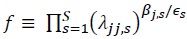in (1) and 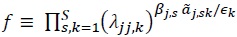in (2) and totally differentiating (1) and (2) to get a first-order Taylor approximation of the change in GTA obtains for the model without intermediates:

and for the model with intermediates:

As the derivative is defined to be a constant only over an infinitely small interval, for numerical implementation to be as precise as possible the observed changes in the variables λ_jj,k, β_j,s and are divided into small intervals and the partial derivatives evaluated over those intervals.19

Table 2 decomposes the changes in GTA into changes in λ and β in the model without intermediates and into changes in λ, β and ã in the model with intermediates. The contributions of the elements are based on the approximations just discussed, but applied to the observed total change in GTA. On average, for the world as a whole, the bulk of the changes in GTA is due to changes in the share of expenditure on domestically produced goods and services. The contribution of ã is on average the same as that of β. However, there is heterogeneity across countries in the importance of the three channels. In the model without intermediates, for example, there is the Netherlands with a negative contribution of β dominating a positive contribution of λ, Slovenia with a negative contribution of β dominated by a positive contribution of λ, Austria with almost equal positive contributions of β and λ, and India with a positive contribution of λ and a negligible negative contribution of β. This heterogeneity across countries is not explained by initial level of development, as was found when running a simple OLS regression of the different components on initial per capita GDP (not reported here).

19)I use 500 intervals for the model without intermediates and 100 intervals for the model with intermediates.

IV. AUTARKY GAINS FROM TRADE AND CHANGES IN TRADE COSTS

Having found that autarky gains from trade (GTA) have on average increased between 1995 and 2006, I proceed to gauge what GTA would have been in 2006 had trade costs in 2006 remained the same as in 1995. This allows me assess to what extent changes in trade costs have contributed to changes in GTA. Notice that the variables λ_jj, λ_jj,s, β_js, e_js and r_js are by definition functions of intranational and international trade (X_ij or X_ijs), at the aggregate or sectoral level. is a function of trade at the sectoral level (X_ijs) as well as intersectoral trade flow (X_ij,ks) The GTA formula for different models share a common grounding in the gravity equation, which explains trade at the aggregate or sectoral level as a function of bilateral trade cost, exporter-specific factor and importer-specific factor. I use the gravity-based CANOVA method proposed by Egger and Nigai (2015) to first obtain unbiased measures of total bilateral trade costs for 1995 (1996) and 2005 (2006), and use the change in trade costs between the two years to obtain counterfactual trade flows for 2005 (2006) at 1995 (1996) trade costs (ie, what trade flows in 2005 would have been if trade costs had remained unchanged from 1995). I then use the counterfactual trade flows to compute GTA for 2005 (2006).20

Before describing the method in more detail, let’s summarize it with some intuition. The GTA formulas come from comparing an observed equilibrium with some trade to a counter factual equilibrium with no trade, where trade costs are prohibitively high. Since the GTA formulas depend only on the observed equilibrium with trade, changes in the observed equilibrium with trade over time affect GTA. The changes in the observed equilibrium with trade over time are all ultimately functions of changes in trade flows, which are in turn functions, in part, of changes in trade costs. If the cost of moving to autarky has increased over time since dependence on imports has increased (which is what the increase in GTA essentially implies in the one-sector model), it begs the question as to what extent trade costs directly explain changes in the importance of imports relative to expenditure on domestic goods and services vis-à-vis exporter-specific factors like supply capacity and importer-specific factors like taste. To answer this question, we first need to perform a counterfactual analysis, unrelated to autarky: what would trade flows have been at year t if trade costs had been the same as at year t₀(< t))? This we do with the aid of the CANOVA method. These counterfactual trade flows are then used to compute counterfactual autarky gains from trade, ie, the gains from trade associated with movement to autarky at year t had trade costs remained the same as at year t_o.

1. The method

The CANOVA method works with any generic gravity model, where bilateral imports of country i from j at time t are expressed as:

where δ_ij,t represents country-pair-time-specific trade costs and ζ_j,t and μ_i,t are, respectively, exporter-time- and importer-time-specific variables. δ_ij,t can be interpreted as δ_ij,t ≡ σ ln τ_ij,t where τ_ij,t is ad-valorem trade costs, and σ < 0 is the partial effect of bilateral trade costs or trade elasticity. ζ_j,t and μ_i,t are implicit functions of bilateral trade costs through the resource constraint (with deficit parameter D_j,t):

The structural country-time parameters can be expressed as:

The first step of the CANOVA method delivers unbiased estimates of δ_ij,1995 and δ_ij,2005. A key feature of this method is that the trade costs are not parameterized and hence avoids “residual trade cost bias”, which arises from the endogeneity of country-time-specific variables to residual trade costs. This method uses, for each year, J² observations on aggregate bilateral sales underlying equation (3) and explains them by J(J − 1) country-pair specific indicators for all pairs i ≠ j, J exporter indicators and J importer indicators, subject to the GE constraints in (5).21 The parameters on country-pair specific indicators yield δ_ij,t (δ_jj,t = 0 for all j, t, i.e., intranational trade costs are normalized to zero), which are unbiased since all trade costs—parameterized as well as residual—are always treated jointly and properly accounted for (Egger and Nigai, 2015). Then, utilizing the model structure in (3)-(5) and using as data the change in bilateral trade costs, Δδ_ij ≡ δ_ij,1995 − δ_ij,2005, the trade flows observed in 2005, X_ij,2005, the trade deficits observed in 2005, D_i,2005, while keeping trade deficits in the counterfactual equilibrium constant relative to world income and expenditures, one can obtain X_ij,2005(δ_ij,1995), ie, the trade flow in 2005 had trade costs remained unchanged at 1995 levels.22 With counterfactual trade flows at hand, I can compute counterfactual autarky gains from trade, GTA²⁰⁰⁵ (δ_ij,1995), ie, gains from trade associated with movement to autarky in 2005 had trade costs remained the same as in 1995.

Two issues must be tackled when applying this method. The first concerns models with intermediate goods. Computing counterfactual GTA for models with intermediates is tricky since some variables are a function of not just trade at the sectoral level but also intersectoral trade and the ratio of value added to gross output. The gravity equation on which the GTA formula for models with intermediate goods are based is at the sectoral level (X_ijs), not at the intersectoral level (X_ij,ks). It is therefore not straightforward to obtain counterfactual values of, say, and b_jk within the present gravity framework. As a compromise, within the class of models incorporating intermediates, I only consider perfect competition, and fix at 2005 values when computing counterfactual GTA. A caveat of doing so is that we are ignoring the potential contribution of changes in trade costs to changes in the technology matrix as captured by the input-output table. The second issue concerns zero flows. About 7 percent of country pairs have zero flows on average at the sectoral level in 1995 and 6 percent in 2005. At the aggregate level, there is positive trade between all countries in the sample, so this is not a concern in the one-sector model. Zero flows are far more important in services sectors relative to non-services sectors, with the share of zero flows about one fifth or above in Construction, Real Estate, Education, Health and Social Work, Retail Trade, and Hotels and Restaurants in 1995, although it declined moderately in 2005. It is not straightforward to handle zero trade flows in the CANOVA framework. I employ two different solutions. The first is to assume no change in trade costs between a country pair between 1995 and 2005 whenever bilateral trade is zero in at least one of the two years. This returns zero counterfactual trade flow whenever observed 2005 trade flow is zero, irrespective of whether trade flow in 1995 is zero or not. The second solution is to add a tiny number (say, 0.000001) to all trade flows and then perform CANOVA. The two different approaches to handle zero flows yield very similar results. I only present results using the first approach.

2. Results

As we expect trade costs to have fallen on average during 1995-2006, we would expect GTA in 2006 with trade costs fixed at 1995 levels to be lower than GTA in 2006 based on observed data. That is what we find, and the differences are statistically significant (Table 3). Notice that since both observed GTA and counterfactual GTA share the same exporter- and importer-specific factors and differ only in trade costs, the difference can be attributed to changes in trade costs that occurred during 1995-2006. In the one-sector model, GTA in 2006 was 34% higher than it would have been without changes in trade costs. In the multisector model with perfect competition, it is 59% higher. In the multisector model with monopolistic competition, it is 101% higher. In the multisector model with intermediates and perfect competition, it is 33% higher.

The intuition behind the substantially higher increase in GTA due to changes in trade costs in the monopolistic competition model relative to the perfect competition model, both without intermediates, is that scale economies and associated variety gains from trade have a role in the former and none in the latter, and changes in trade costs affect these channels considerably. The relative lower increase in GTA due to changes in trade costs in the multisector model with intermediates and perfect competition should be interpreted with caution because we have constrained the input-output structure to be invariant to trade costs, in the absence of a clear-cut method to compute changes in the input-output structure arising from changes in trade costs.

The difference between the numbers in the row “Difference” in Tables 3 and 1 is equivalent to the difference between GTA for 1995 using observed data and GTA for 2006 using counterfactual data. This difference in differences arises from possible changes in exporter- and importer-specific factors over that period, as trade costs have been kept constant. The difference is positive in the one-sector model and the two multisector models without intermediates, and negative in the multisector model with perfect competition and intermediates. However, it is significantly different from zero, at conventional levels, only in the one-sector model (5% level) and the multisector monopolistic competition model without intermediates (1% level). In these two models, the positive difference (in differences) implies that changes in exporter- and importer-specific factors, over and above changes in trade costs, have detracted from the welfare cost of autarky.

Figures 3-6 compare the observed GTA and counterfactual GTA for all countries in the sample for the one-sector model and each of the three multisector models. The dashed and dotted lines are the averages, the same as in Table 3. These figures suggest that changes in trade costs have led to an increase in autarky gains from trade for most countries. Regressing the ratio of observed GTA to counterfactual GTA on initial (log) per capita GDP, we find a statistically significant negative relationship for the one-sector model (coefficient: -0.2) and perfect competition models (with and without intermediates; coefficient: -0.3). The increase in autarky gains from trade due to changes in trade costs has been higher the lower the initial income. The relationship is negative but not statistically significant for the monopolistic competition model.

20)The results for gains from trade are based on averages for 1995-96 and 2005-06.

21)Computing bilateral trade costs separately for each year is in line with an exercise in Egger and Nigai (2015) wherein bilateral trade costs are estimated separately for two different years before gauging the contribution of the changes in those trade costs to the changes in trade flows between the two years.

22)Note that in the CANOVA approach, intranational trade costs are assumed to be zero, and hence do not change over time. Despite this, we can still expect intranational trade to be different at the counterfactual equilibrium than at the observed equilibrium due to general equilibrium effects captured in a structural gravity framework.

V. CONCLUSION

This paper analyzes changes in autarky gains from trade between 1995 and 2006, a period of rapid globalization. It uses state-of-the-art micro-founded quantitative trade models based on the gravity equation, as developed in Arkolakis et al. (2012) and Costinot and Rodriguez Clare (2014). It finds that the cost of moving to autarky has increased, by over 40% on average. Through a decomposition of the changes in autarky gains from trade, it finds that changes in the share of spending on domestic goods and services explain most of those changes, with a limited role for reallocations of spending across sectors with differing trade elasticities. Estimating trade costs using a recently introduced method of structural estimation of the gravity model that accounts for residual trade cost bias—an ANOVA-type estimation due to Egger and Nigai (2015)—the paper also finds that average autarky gains from trade at the end of the decade where 60-100% higher than what they would have been had trade costs remained unchanged from the beginning of the decade. Revealing cross-country heterogeneity in the results, the paper indicates that rigorously explaining the heterogeneity is a worthwhile line of enquiry for future research.

APPENDIX23

23)Figures in the Appendix are based on the author’s computation using trade flows from the World Input-Output Database, per capita GDP from the CEPII database and trade-to-GDP ratio from the World Development Indicators.