

- EAER>
- Journal Archive>
- Contents>
- articleView
Contents
Citation
| No | Title |
|---|
Article View
East Asian Economic Review Vol. 23, No. 2, 2019. pp. 169-202.
DOI https://dx.doi.org/10.11644/KIEP.EAER.2019.23.2.360
Number of citation : 0View
127
Download
68
Specialization, Firm Dynamics and Economic Growth
|
|
Korea Institute for Industrial Economics and Trade (KIET) |
|---|---|
|
|
China Institute of Finance and Capital Market |

Abstract
Productivity in agriculture or services has long been understood as playing an important role in the growth of manufacturing. In this paper we present a general equilibrium model in which manufacturing growth is stimulated by non-manufacturing sectors that provides goods used in both research and final consumption. The model permits the evaluation of two policy options for stimulating manufacturing growth: (1) a country imports more non-manufacturing goods from a foreign country with higher productivity and (2) a country increases productivity of domestic non-manufacturing. We find that both policies improve welfare of the economy, but depending on the policy the manufacturing sector responses differently. Specifically, employment and value-added in manufacturing increase with policy (1), but contract with policy (2). Therefore, specialization of the import nonmanufactured goods helps explain why some Asian economies experience rapid growth in the manufacturing sector without progress in other sectors.
JEL Classification: F11, F43, F63
Keywords
Firm Heterogeneity, Firm Innovation, Economic Growth, Specialization, Unbalanced Sector Growth
I. INTRODUCTION
A large literature in economic development has discussed the important role that productivity in agriculture or services has played for the growth of manufacturing and the economy as whole.1 However, empirical evidence from major Asian economies (including Japan, Korea and China) is inconsistent with this literature. These countries achieved unprecedented growth in the manufacturing sector without significant productivity improvement in other sectors.2 This raises a question: is high productivity in other sectors necessary to achieving rapid manufacturing growth?
To answer this question, we build a general equilibrium model comprising two sectors: manufacturing and non-manufacturing. In the manufacturing sector, heterogeneous firms grow endogenously by investing in innovation. The non-manufacturing sector meanwhile provides a non-manufactured good, which is a source of the final good in either innovation investment or final consumption. To test the model, we weigh two policy choices that exogenously expand the output of the non-manufactured good. The first exogenous change involves increasing the productivity of the firm in the domestic non-manufacturing sector, a structural transformation emphasized in previous literature. The second change consists of expanding imports of the non-manufactured good from a foreign country that has higher productivity in the non-manufacturing sector. We then study how these two exogenous changes affect the innovation decisions of firms and economic growth in the manufacturing sector.
The model predicts that both exogenous policies increase overall economic welfare due to the falling price of the non-manufacturing good, but predicts contrary outcomes in the manufacturing sector. When the economy imports more non-manufactured goods from foreign countries, firms in the manufacturing sector have an increased incentive to conduct innovation because of the lower price of non-manufactured goods. As the rate of productivity increases, labor moves from the non-manufacturing sector to the manufacturing sector. On the other hand, when the policy entails increasing the productivity of the domestic firm in the non-manufacturing sector, the productivity of firms in the manufacturing sector increases relatively slowly and can even decrease depending on parameters in the model. In this last case, labor can even shift from the manufacturing sector to the non-manufacturing sector.
This consequence has an intuitive explanation. Both policy changes reduce the price of the non-manufactured good and give firms in the manufacturing sector more incentive to innovate. However, if the economy increases the productivity of the firm in the non-manufacturing sector, this firm will hire more labor. Thus, this change increases the demand for labor – and labor cost – throughout the economy. Higher costs lower the profitability of firms in the manufacturing sector and cause them to pursue less innovation. On the other hand, importing more non-manufactured goods benefits firms in the manufacturing sector by lowering the price of the non-manufactured good, but has no impact on labor costs. This stimulates innovation and growth in the manufacturing sector, and encourages manufacturing specialization in the economy as a whole.
The motivation for this research is the experience of Asian economies such as Japan, Korea and China. Each experienced unprecedented rapid economic growth even as growth in non-manufacturing sectors lagged. Figure 1 shows changes in labor productivity normalized as of 1965 by sector in Asian economies and the United States from 1965 to 2000. As shown by the data, the increase in labor productivity of the manufacturing sector (marked by solid lines) in Asian economies such as Korea and China is relatively prominent compared to that of non-manufacturing industries (marked by dotted lines). In the United States, however, the increase in labor productivity in the manufacturing sector outweighs that in the non-manufacturing sector, but the difference is barely noticeable. In Japan, labor productivity in the manufacturing and non-manufacturing sectors has been increasing since the 1990s, but up to the 1980s – generally considered a high-growth period – a pattern similar to that of the other Asian economies is observed.
For more specific instance, consider the pattern of Korean economic growth. From 1977 to 1988, Korean total labor productivity increased by 6.6% yearly, while total labor productivity in the manufacturing sector increased by 8.9% yearly and that in other sectors stagnated.3 Even compared to the respective sectoral growth rates of the EU and US during the same time period, the manufacturing sector in Korea grew faster while the other sectors did not. The growth miracle in Japan, which experienced rapid economic expansion before Korea, demonstrated a similar pattern. Ito and Weinstein (1996) show that the primary source of Japan’s rapid growth was the high rate of productivity growth in the manufacturing sector and the shift of resources to the manufacturing sector is observable during the rapid growth period.
Consistent with our modeling framework, we also observe a significant increase in imports of non-manufactured goods during the same period in Korea. From 1977 to 1988, agriculture and raw materials imports increased by 16.8% yearly and services imports increased by 18.5% annually.4
The economy imported more goods from non-manufacturing sectors where domestic production grew slowly. These facts suggest that comparative advantage in specific industries led to unbalanced growth, where some sectors of the economy improved while other stagnated.5 This differs from the pattern exhibited by the developed countries during their structural transformations.
We also use the model to conduct several numerical experiments. We obtain three findings with implications for national development. First, we show that allowing the import of more non-manufactured goods from abroad makes firms in the manufacturing sectors grow more rapidly than increasing the productivity of the non-manufacturing sector quantitatively. Second, we show that the growth of the manufacturing sector is slower with higher productivity in the non-manufacturing sector when the economy allows the imports of more non-manufactured goods. Lastly, we find that a larger economy derives a greater increase in welfare from a policy that focuses on increasing domestic productivity of the non-manufacturing sector and developing both sectors in tandem.
Our research is related to previous works in economic growth and development. Specifically, it is in line with the development literature that attempts to explain how a country initiates manufacturing sector growth and the role of other sectors in that process. Matsuyama (1992), Kögel and Prskawetz (2001) and Gollin, Parente, and Rogerson (2002) emphasize the importance of the development of the agriculture sector in allowing for labor or other resources to be transferred to the manufacturing sector. Moreover, other literature such as Francois (1990), Neusser and Kugler (1998), Francois and Hoekman (2010) and Kehoe and Ruhl (2012) emphasize the importance of the development in the service sector, including the provision of financial or business services, as intermediates for manufacturing. While the previous works consider the development of the non-manufacturing sector as the only determinant in the production of non-manufacturing goods, we consider the additional alternative of imported non-manufacturing goods embedded with better technology.
Our work is related to the broad range of literature in endogenous growth that incorporates endogenous R&D decisions in driving economic growth as in Romer (1990), Aghion and Howitt (1992) and Grossman and Helpman (1993).6 The success of innovation is stochastic as in Griliches (1979) and Ericson and Pakes (1995). We incorporate endogenous innovation decisions of firms in the manufacturing sector similar to Klette and Kortum (2004), Lentz and Mortensen (2008) and Atkeson and Burstein (2010). Finally, the model is closely related to that of Atkeson and Burstein (2010) which incorporates firm-level innovation decisions. While they consider symmetrical countries to focus on gains from trade, we focus on growth of developing countries by considering an asymmetric cases with a small open economy. Because our model features two industries, specialization is a key mechanism to evaluate the effects of two-policy changes.
At first glance, the main thrust of our work may appear to diverge from the results of prominent research on the Asian economic miracle, but it is actually complementary.7 Superficially, our emphasis on the importance of imports in non-manufacturing sectors may seem to contradict previous research that assigns great significance to export-driven growth in Asian economies.8 But in fact our research documents how imports in the non-manufacturing sectors led to increases in manufacturing exports and productivity. Our work focuses on explaining how the manufacturing sector grew and exports increased without increased productivity in the non-manufacturing sectors. Seen in this light, our work complements previous studies that stressed the importance of export-driven growth in East Asia.
A recent work by Gersbach, Schneider, and Schneller (2013) evaluates the effects of similar policies. They argue that if an economy imports leading technologies from foreign countries instead of investing in public research, domestic innovation suffers. The main findings of our research seem to contradict this, but in their work, openness to foreign technology discourages the optimization of domestic innovation because foreign technology substitutes domestic technology. In our model, however, there are two sectors, and openness to foreign technology means that an economy imports more non-manufactured goods. Non-manufactured goods as a part of research goods complements innovations in the manufacturing sector. This difference accounts for the seemingly contradictory result produced by our model.9
The remainder of the paper is organized as follows. Section 2 describes a two-sector general equilibrium model where firms in the manufacturing sector grow endogenously and the non-manufacturing sector provides parts of research goods for firms in the manufacturing sector for use in developing innovations. In Section 3, we demonstrate how the two policies result in different consequences, especially in the manufacturing sector. In Section 4, we test the model and describe the implications carried by the results as they relate to the development path of different countries. Section 5 is the conclusion.
1)The literature highlights that increases of productivity in the agriculture sector are an essential condition to reallocate labor from the agriculture sector to the manufacturing sector and to initiate manufacturing sector growth on structural transformation. See
2)See
3)We choose this period because the share of Korean labor in the manufacturing sector increased until 1988. Extending the time period to 1970 does not affect the conclusion. We exclude electricity, gas and water supply. However, this sector constitutes a small share of the total economy.
4)World Development Indicator.
5)We use balanced and unbalanced growth terminology from
6)We use a model where labor is the only input following the previous literature, so productivity determined by R&D investment is labor productivity, which could be increased by increases in other inputs such as capital accumulation as well as TFP. In this regard, it does not conflict with previous studies, e.g.
7)We appreciate the comments of a referee on the need for this discussion.
8)Regarding the relationship between trade and economic growth,
9)While we focus on endogenous growth in manufacturing related to productivity in the non manufacturing sector in a developing country,
II. MODEL
1. Environment
We consider a small open economy surrounded by one continent. The economy has two industrial sectors: manufacturing and non-manufacturing respectively. We assume that goods in manufacturing are perfectly tradable but goods in non-manufacturing are only partially tradable. In the manufacturing sector, firms are heterogeneous in terms of productivity and they can grow endogenously by investing in R&D while there is a homogeneous firm with a productivity in the non-manufacturing sector.10 There is a measure L of infinitely lived homogeneous households in the economy who only value consumption and are endowed with one unit of labor.
2. Manufacturing sector
There is a continuum number of varieties between 0 and N·K produced from either (0,
There are two possible states for a firm’s productivity for each variety, indexed by  The firm uses labor

Output from firms in the manufacturing sector is aggregated through integration with other varieties in the same sector. We call the good which is aggregated by all varieties, denoted by

The small open economy produces variety from (0,
1) Firm innovation
A firm in the manufacturing sector can grow endogenously by investing in R&D to boost future productivity. The final goods variable

2) The manufacturing firm’s problem
The objective of the firm to maximize its value is determined by the sum of current and future values. From the assumption of a small open economy, each individual firm takes the total market size for the manufacturing sector denoted by
A firm with productivity index z can be solved by the following recursive problem.

s.t.

where  is the profit variable that determines the firm’s current value,
3. Non-Manufacturing Sector
The non-manufacturing sector consists of perfectly competitive producers and perferctly-competitive aggregators. A representative firm in the non-manufacturing sector uses labor with constant return to scale production technology and produce non-manufactured goods.
The production function of the firm in the non-manufacturing sector is:

where
Since the non-manufactured good is partially tradable, some of the foreign non-manufactured goods are also available in the domestic market. However, the imported non-manufactured goods and domestic non-manufactured goods are not perfect substitutes. The elasticity of substitution between the two types of non-manufactured goods is
Final non-manufactured goods producers are also built into the model by aggregating non-manufactured goods from both domestic and foreign sources. And both domestic and foreign non-manufactured goods are aggregated into final non-manufactured goods via the following function,

Here
4. Final Good Sector
The final good producers are perfectly competitive producers who use manufactured goods bundles (
The production function of final good production is taken as follows:

The final output is used in consumption and making R&D investments.
5. Households
stand-in consumer is endowed with


Here,  is the expected dividend from firms in the manufacturing sector.
The consumer does not value leisure in our model, so he devotes all his labor endowment into production. Nor does the consumer accumulate any capital, consuming the exact same amount of consumption goods for each period following the permanent income hypothesis.
6. Equilibrium
A stationary recursive equilibrium is a list of aggregate state variables, the distribution of firms’ productivity {
a list of prices:

and a list of decision functions:
a)
b)
c)
d)
e)
and an updating rule for the state variables:

such that
1) The consumer takes wages as given, future dividends, and the other prices. The consumer maximizes lifetime utility through consumption equal to life-time income.
2) Firms in the manufacturing sector take the demand function and the wage as given, choosing
3) The firm in the non-manufacturing sector takes prices as given and produces
4) The non-manufacturing aggregator takes prices as given and it produces final non-manufactured goods,
5) The final aggregator takes prices as given and it produces a final output,
6) How to aggregate each good is consistent with the updating rule of
7) All market clearings and the trade balance conditions hold.
7. Equilibrium Results
1) Non-manufacturing sector:
Since the non-manufacturing sector is perfectly competitive, the price of the non-manufactured good will be equal to the firm’s marginal unit cost:

The non-manufacturing aggregator combines both domestic and foreign non-manufactured goods into final non-manufactured goods using CES technology. Given  as the price of the non-manufactured good imported, its unit cost for producing non-manufacturing goods in the equilibrium will be:

which equals the equilibrium price for the non-manufactured goods.
Then the demand for domestic non-manufacturing inputs should satisfy:

which equals the total wages paid to the workers in the domestic non-manufacturing sectors,
On the other hand, the total amount of non-manufactured goods from a foreign country is:

2) Manufacturing sector
A firm with productivity z in the manufacturing sector maximizes its profit under the monopolistic competition, given the world market size for manufacturing goods,
In the equilibrium, the demand for labor at manufacturing firms with productivity index z given wage(

And its profit will be:

The innovation cost function is  for simplicity in writing. In the equilibrium, the value function of a manufacturing industry firm is:


The optimal innovation cost

3) Final aggregation sector
Since the production function is Cobb-Douglas and the final good sector is perfectly competitive, the two first order conditions give the equilibrium demand for manufactured goods and non-manufactured goods:

And correspondingly, the equilibrium price of the final goods will be

4) Market clearing
The labor demand for the manufacturing sector and the non-manufacturing sector are

The final good market is cleared for each period:

The trade balance condition is

Since the country is a small country, the above euation could be trasformed to

Futhermore, from  we can derive the following condition

10)We are particularly interested in the growth miracle in East Asian countries.
11)The main goal of the paper is not to analyze a change of the number of firms but growth in the size of incumbent firms. If we allow the free entry condition to determine the number of firms endogenously, we can have different size in the manufacturing sector instead of individual firms’ growth patterns.
12)Combining Equation (15) with Equation (5), we can derive the final demand for the firm at equilibrium.
13)h is a parameter to determine the innovation productivity.
14)Where 
III. COMPARATIVE STATICS FOR PARAMETERS θ AND λ
The model equilibrium is characterized by the equilibrium wage and prices. Since a unique equilibrium exists in the model, we conduct an comparative analysis by altering parameters
As we discussed before, a higher
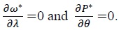
Since the equilibrium (
The equilibrium condition gives us,

We rewrite the market clearing condition for the final goods as

and substitute it into the market clearing condition for labor. Then the equilibrium

Let

We take first order derivatives of the wedge equation with respect to 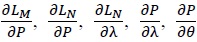 are negative and
  are positive in the equilibrium.

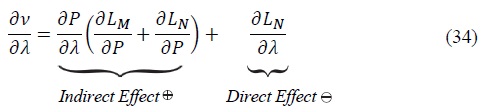
The indirect effect comes from changes in prices. Regardless of whether an economy imports more non-manufactured goods from a foreign country or produces non-manufactured goods domestically with higher productivity, it can use cheaper non-manufactured goods to reduce the costs of final goods and innovation. So firms in the manufacturing sector grow and attract labor.
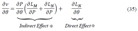
Whereas the direct effect of the two possible parameter changes moves the equilibrium in opposite directions. When the economy can import more non-manufactured goods from a foreign country, domestic non-manufacturing goods are replaced by the foreign non-manufactured goods. Then, labor demand in the non-manufacturing sector decreases resulting in a surplus labor supply. On the other hand, when the economy increases productivity of the non manufacturing sector, labor demand in the non-manufacturing sector increases, resulting in labor shortages.
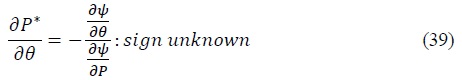
From the three equations above, the implicit function theorem tells us that

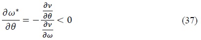
We do the same thing for

As similar to wages, we argue that when an economy imports more non-manufactured goods, represented by an increase in
15)Government policies affecting
16)Considering labor productivity in the model, policies that enhance productivity in the non-manufacturing sector,
IV. QUANTITATIVE ANALYSIS
1. Extended Model for Simulation
In this section, we extend the baseline model to an infinite number of possible productivity levels for firms in the manufacturing sector in order to a conduct quantitative analysis. Following Atkeson and Burstein (2010), a firm in the manufacturing sector invests

exp(Δ) is the productivity difference between the two adjacent productivity indexes. Now
For conducting some simulation results, we parameterize the model. We provide the values of the parameters used in Table 2.17
2. Simulation Analysis
Using the extended model, we will conduct some counterfactual analysis. We focus especially on two exogenous changes in
In Experiment 1, we show Proposition 2 quantitatively with heterogeneity in firms’ productivity but with multiple productivity levels using the extended model. For the experiment, we start from a specific (θ, λ) pair as (0.1, 0.1). We do not construct an explicit cost function for the two policies. To consider changes wrought by the two policies comparably, first we change θ to 0.3 and calculate the changes in household welfare. From the change in household welfare, we find the change in λ that guarantees an equal change in household welfare, λ = 0.273. We then compare the changes in each policy, which increase
Figure 2 says that the increase in  Although both changes were designed to result in identical changes in welfare, the change in
The quantitative result is consistent with Proposition 2 in Section 2 which comprises the analytical result with two possible productivity levels. As we explained in the model, this is related to specialization. Due to lower prices of non-manufactured goods, both parameter changes incentivize innovation. However, an increase in
For Experiment 2, we start from two different pairs (
Quantitatively, a change in
The result implies that when a country has very low productivity across all industries, the manufacturing sector seizes comparative advantage through the opening if the non-manufacturing sector. The county then experiences rapid growth and specializes in the manufacturing, as was the case of “miracle” economies in Asia. However, when a country’s income levels increase due to higher productivity in the non-manufacturing sector, then comparative advantage evaporates. This can explain why manufacturing firms in a developing country can grow extremely rapidly compared to those in a developed country.
In Experiment 3, we describe the impact of different policies based on the size of the countries in which they are implemented. We start from a specific (
The result carries the implication that a larger country could achieve rapid growth in the manufacturing sector through specialization. However, in terms of overall benefits to welfare, gains large countries reap by opening the non-manufacturing sector relative to increasing their own productivity in the non-manufacturing sector are smaller, owing to their size. This tells us that balanced growth that includes increasing productivity in the non-manufacturing sector as well is a necessary policy for larger countries.
Eichengreen, Park, and Shin (2012) analyze historical growth experiences of countries, and have argued that a country experiences a slowdown of economic growth when per capita GDP reaches $13,000 per year, the so-called “Middle income trap”. To avoid it, they stress increasing productivity in the non-manufacturing sector. From a historical analysis of other countries, They argue that China too will spring the trap when its income level reaches $13,000. However, our model suggests that it is necessary that lowincome countries increase productivity in the non-manufacturing sector for better welfare returns; as China is much bigger than other low-income countries its experience is fundamentally different.
17)Our goal is not to give an accurate quantitative analysis for the sake of policy-making but to describe the implications carried by different policies. Accordingly, parameters were not precisely calibrated.
18)An evaluation of which of the two policies is better for overall growth would require a more precise calibration. This paper instead focuses on the comparison of manufacturing firm dynamics in responding to policies. A quantitative assessment of the effects of both policies on overall economic growth is a subject for future research.
V. CONCLUSION
In this paper, we build a model with two sectors. In it, the manufacturing sector grows endogenously and the non-manufacturing sector provides goods used for both research and final consumption, stimulating innovation at firms in the manufacturing sector. Through the model we examine the effects of two exogenous changes that expand the output of goods in the non-manufacturing sector. The first policy increases domestic productivity in the non-manufacturing sector. The second increases imports of non-manufactured goods from a foreign country with higher productivity. Even though both changes improve the welfare of the economy, both theoretically and quantitatively, we show that effects on the manufacturing sector are different. Our model predicts that the latter change makes manufacturing firms grow faster and attract more labor than the former. Based on our results, we argue that specialization through importing non-manufactured goods contributes to Asian economic growth, but not increasing productivity in the non-manufacturing sector, as the previous literature on structural transformation has emphasized.
We also conduct experiments using the model that have implications for economic development. Our experiments suggest that manufacturing growth is slower with higher productivity in the non-manufacturing sector when the economy allows imports of more non-manufactured goods. This implies that in terms of manufacturing growth, a developing country has greater incentive than a developed country to specialize in manufacturing by importing the non-manufactured goods it consumes because its productivity in the non-manufacturing sector is lower. Furthermore, a larger economy realizes larger welfare gains from increasing the domestic productivity of the non-manufacturing sector and developing both sectors in a balanced way. This result carries obvious implications for the growth of the Chinese economy. A similar pattern of economic growth as seen in Japan or Korea could guarantee fast growth in Chinese manufacturing.19 In terms of welfare, however, China might see slower improvements relative to that of Japan and Korea because China is much larger than either country.
Some assumptions of the model did not address a number of issues. For example, the model in this study assumes the free mobility of labor between two sectors, equalizing wages between them. As a result, labor always moves to manufacturing when importing non-manufacturing goods and the transition has a positive effect on manufacturing growth. In practice, however, these mechanisms would vary depending on wage differences between the sectors. This would require a more complex labor market in the model accurately calibrated to the actual data. Using such a model, it would be possible to study labor mobility during the structural transformation leading to the economic growth period and also analyze changes in prices and wages of goods between sectors. We leave this to future research.
19)
Tables & Figures
Figure 1.
Sectoral Labor Productivity

Note: We calculate labor productivity by sectoral value added in 2005 prices divided by employment based on
Source: Groningen Growth and Development Centre. <
Table 1.
Growth Rate of Labor Productivity from 1977-1988

Note: We calculate growth rate of labor productivity using gross value-added per hour from EU KLEMS.
Table 2.
Parameters of the Model for the Simulations

Note:
Figure 2.
Distribution of Firm Productivity after Increases in

Figure 3.
Distribution of Firm Productivity after Increases in λ on Different

Figure 4.
Relation between λ and Labor

APPENDIX: PROOF OF LEMMA AND PROPOSITION
In the equilibrium, the distribution of firm productivity

So

and

given the expression of labor engaged in the manufacturing sector in the equation (22), and apply the chain rule:


Step 2:

Let


Then

We can easily show that 
From the definition of dividend,

By the equation (16) and (19)

So,

Since we know 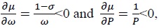 and through the chain rule:


Since the total demand of labor equals the sum of demand from the manufacturing and non-manufacturing sector.

1. Labor market clearing condition: LD = L
Since
All the equilibrium P satisfying the labor market clearing condition must monotonically decreasing with equilibrium wage level
2. Final good clearing condition under optimal choice of aggregating firms gives:

All the equilibrium P satisfying the final good and intermediate good clearing condition must monotonically increase in equilibrium wage level
So, the (
And from this wage price level pair, the entire equilibrium under this price system is unique.
Direct Effect:
By the equation (23)

As 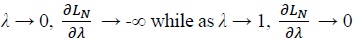
Indirect Effect:
By the equation (21), (12), (22) and (23)

Since 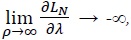 there exist an
  for all
  such that
which implies that there is a correspondence of 
Similarly,

As 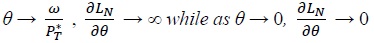
Therefore 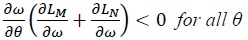
Since 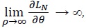 there exist an
  such that

This implies a correspondence of 

The intersecting points of this correspondence would satisfy our requirement.
 there exists some point satisfied the condition chracterized by lemma 2.
Starting from the these (
When 
Since the equilibrium 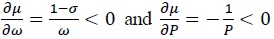
Appendix Tables & Figures
References
-
Aghion, P. and P. Howitt. 1992. “A Model of Growth Through Creative Destruction,”
Econometrica , vol. 60, no. 2, pp. 323-351.
-
Atkeson, A. and A. T. Burstein. 2010. “Innovation, Firm Dynamics, and International Trade,”
Journal of Political Economy , vol. 118, no. 3, pp. 433-484.
-
Bosworth, B. and S. M. Collins. 2008. “Accounting for Growth: Comparing China and India,”
Journal of Economic Perspectives , vol. 22, no. 1, pp. 45-66.
-
Diao, X., Roe, T. and E. Yeldan. 1999. “Strategic Policies and Growth: An Applied Model of R&D-driven Endogenous Growth,”
Journal of Development Economics , vol. 60, no. 2, pp. 343-380.
-
Eichengreen, B., Park, D. and K. Shin. 2012. “When Fast-growing Economies Slow Down: International Evidence and Implications for China?,”
Asian Economic Papers , vol. 11, no. 1, pp. 42-87.
-
Eichengreen, B., Perkins, D. H. and K. Shin. 2012.
From Miracle to Maturity: The Growth of The Korean Economy (Harvard East Asian Monographs) . Cambridge, MA: Harvard University Asia Center. -
Ericson, R. and A. Pakes. 1995. “Markov-perfect Industry Dynamics: A Framework for Empirical Work,”
Review of Economic Studies , vol. 62, no. 1, pp. 53-82.
-
Francois, J. F. 1990. “Trade in Producer Services and Returns Due to Specialization Under Monopolistic Competition,”
Canadian Journal of Economics , vol. 23, no. 1, pp. 109-124.
-
Francois, J. and B. Hoekman. 2010. “Services Trade and Policy,”
Journal of Economic Literature , vol. 48, no. 3, pp. 642-692.
-
Gersbach, H., Schneider, M. T. and O. Schneller. 2013. “Basic Research, Openness, and Convergence,”
Journal of Economic Growth , vol. 18, no. 1, pp. 33-68.
-
Gollin, D., Parente, S. and R. Rogerson. 2002. “The Role of Agriculture in Development,”
American Economic Review , vol. 92, no. 2, pp. 160-164.
-
Griliches, Z. 1979. “Issues in Assessing the Contribution of Research and Development to Produc tivity Growth,”
Bell Journal of Economics , vol. 10, no. 1, pp. 92-116.
-
Grossman, G. M. and E. Helpman. 1993.
Innovation and Growth in The Global Economy . Vol. 1. Cambridge, Mass: MIT Press. -
Ito, T. and D. E. Weinstein. 1996. “Japan and the Asian Economies: A “Miracle” in Transition,”
Brookings Papers on Economic Activity , vol. 1996, no. 2, pp. 205-272.
- Kehoe, T. J. and K. J. Ruhl. 2012. Why Have Economic Reforms in Mexico Not Generated Growth?. NBER Working Paper, no. 16580.
-
Klette, T. J. and S. Kortum. 2004. “Innovating Firms and Aggregate Innovation,”
Journal of Political Economy , vol. 112, no. 5, pp. 986-1018.
-
Kögel, T. and A. Prskawetz. 2001. “Agricultural Productivity Growth and Escape From the Malthusian Trap,”
Journal of Economic Growth , vol. 6, no. 4, pp. 337-357.
-
Krueger, A. O. 1990. “Asian Trade and Growth Lessons,”
American Economic Review , vol. 80, no. 2, pp. 108-112. -
Kuznets, S. 1966.
Modern Economic Growth: Rate, Structure, and Spread . London and New Haven: Yale University Press. -
Lentz, R. and D. T. Mortensen. 2008. “An Empirical Model of Growth Through Product Innovation,”
Econometrica , vol. 76, no. 6, pp. 1317-1373.
-
Matsuyama, K. 1992. “Agricultural Productivity, Comparative Advantage, and Economic Growth,”
Journal of Economic Theory , vol. 58, no. 2, pp. 317-334.
-
Neusser, K. and M. Kugler. 1998. “Manufacturing Growth and Financial Development: Evidence from OECD Countries,”
Review of Economics and Statistics , vol. 80, no. 4, pp. 638-646.
-
Rauch, J. E. 1997. “Balanced and Unbalanced Growth,”
Journal of Development Economics , vol. 53, no. 1, pp. 41-66.
-
Romer, P. M. 1990. “Endogenous Technological Change,”
Journal of Political Economy , vol. 98, no. 5, part 2, pp. S71-S102.
- Sachs, J. D. and A. M. Warner. 1995. Natural Resource Abundance and Economic Growth. NBER Working Paper, no. 5398.
-
Timmer, M., De Vries, G. J. and K. De Vries. 2016. Patterns of Structural Change in Developing Countries. In Weiss, J. and M. Tribe. (eds.)
Routledge Handbook of Industry and Development . New York: Routledge. Taylor & Francis. pp. 65-83. -
Westphal, L. E. 1990. “Industrial Policy in an Export-propelled Economy: Lessons from South Korea’s Experience,”
Journal of Economic PerspectivesI , vol. 4, no. 3, pp. 41-59.
-
Young, A. 1995. “The Tyranny of Numbers: Confronting the Statistical Realities of the East Asian Growth Experience,”
Quarterly Journal of Economics , vol. 110, no. 3, pp. 641-680.