I. INTRODUCTION

The world economy has entered a period of turbulence in the 21st century. Since the launch of the WTO (World Trade Organization) in 1995, the global economy has faced an era of endless competition, as movement of services and capital as well as foreign trade have become free-flowing. Globalization of the world economy has had positive aspects such as productivity improvement and price stability. However, as observed in the global financial crisis, a country’s economic conditions are impacted by financial crisis or recession of other countries. Especially, in the case of a small open economy such as that in Korea, economic analysis without consideration of external economic conditions would not be significant today because it is significantly influenced by economic situations and policies of other major countries.

Therefore, this study examines the effects of economic policies, especially domestic monetary policy, on major domestic macroeconomic variables such as GDP, prices, and won/dollar exchange rates, assuming a two-country open economy model. Analytical methods are based on structural and reduced-form approaches, because results from the two approaches differ according to previous domestic studies. First, the two-country new Keynesian dynamic stochastic general equilibrium (DSGE) model, extending the Lubik and Schorfheide (2006) model, is considered a structural approach for systematic analysis in this study. This structural approach has the advantage of clarifying the direction of causal relationship between variables and enhancing predictability of policy effects. However, since paths through which the policy effect is propagated cannot be modeled without exception, model misspecification is likely to occur. This study also compares effects of the same policy using the reduced-form VAR model with the same variables. The reduced-form approach has the advantage of looking at the direct causal relationship between causal and consequential variables without specifying the specific path to which policy effects are propagated. However, the abbreviated approach has the problem of neglecting reverse causation or unknown outside factors. Estimating the DSGE model is as well-known as estimating the VAR model with cross-equation constraints.

Recently, the DSGE-VAR model has been introduced to systematically mitigate cross-coefficient constraints imposed on the VAR by the DSGE model. This model has an intermediate form of the VAR approximation of the DSGE and the unconstrained VAR. This study will also examine DSGE-VAR as well as DSGE and VAR. In this study, first, impulse response analysis of DSGE, DSGE-VAR, and VAR models reveals how the impact of the domestic interest rate hike dynamically influences domestic GDP, prices, and won/dollar exchange rates during the entire sample period (1990:2-2016:1) and the relatively stable period (1999:2-2007:1). Under the Korean market average exchange rate system, because the daily fluctuation of the won/dollar exchange rate is limited, market information cannot be immediately reflected in the won/dollar exchange rate. Therefore, the autoregressive time series model has a better forecasting power of won/dollar exchange rate than the structural monetary model and the random walk model. However, as the market average exchange rate system moved to the free floating exchange rate system in December 1997 immediately after the currency crisis, not only has it been more difficult to predict the won/dollar exchange rate than before, but also its volatility has increased. This is because the won/dollar exchange rate not only absorbs the ripple effect of domestic monetary policy, but also plays an important role on mechanism of domestic spillover of global macro financial shocks like what happened after the global financial crisis. Korea is a small open economy with a high degree of trade dependence as well as a great deal of financial market opening after the currency crisis. Accordingly, it seems that there is a limit to analyzing the relationship between the domestic monetary policy and the won/dollar exchange rate with the existing theoretical model that explains the exchange rate of developed countries. The paper also compares the explanatory power of these models with marginal data density and in-sample root mean square error (RMSE) criteria.

Impulse response analysis shows that a domestic interest rate hike raises won value in the case of DSGE and DSGE-VAR models, while that in the case of the VAR model without restrictions, it decreases won value. According to the marginal data density standard, DSGE-VAR (μ=1) is superior to DSGE or Bayesian VAR over the sample period. Conversely, according to the in-sample RMSE standard, VARs are superior to DSGE or DSGE-VAR.

This study consists of the following contents. In Section II, I review previous studies related to DSGE, DSGE-VAR, and VAR, and discuss differences from this study. Section III explains the two-country open economy DSGE model that extended the Lubik and Schorfheide (2006) model and examines DSGE and DSGE-VAR estimation methods. Section IV analyzes response of key macroeconomic variables to monetary policy shocks and discusses model excellence based on marginal data density and in-sample RMSE standard criteria. In Section V, the economic meaning implied by this study is examined. Finally, in Section VI, contents of this study are summarized and concluded.

II. LITERATURE REVIEW

The new open economy macroeconomic model (NOEM) developed by Obstfeld and Rogoff (1995) is differentiated from the past international financial model represented by Mundell-Fleming-Dornbusch and is related to the recent trend of monetary economics. It is a model of an open economy that corresponds to a general approach such as the New Keynesian or the New Classical approach. The NOEM model has opened a new chapter in the international finance field from a theoretical perspective, but it took time to analyze these models empirically. For example, Leeper and Sims (1994) estimated the DSGE model using the maximum likelihood estimation method to obtain an empirical model useful for monetary policy analysis, and Schorfheide (2000) developed the Bayesian estimation method as the useful technique to estimate and evaluate the DSGE model when the model misspecification exists. Using this method, Smets and Wouters (2003) estimated an optimal model in Europe that was consistent with time series data. Many DSGE models related to small open economies as well as closed economies have been introduced since this study.

Bergin (2003) estimated a small open economy model using a maximum likelihood framework for the first time. Similar studies include Dib (2003), and Ambler et al. (2004). As Clarida et al. (1999) mentioned, small open economy DSGE models have evolved by extending closed economy New Keynesian frameworks and a representative example is Gali and Monacelli (2005). Lubik and Schorfheide (2007) used a simple version of the model of Gali and Monacelli (2005) to analyze if the central bank responds to exchange rate movement. Adolfson et al. (2004), Del Negro (2003), Justiniano and Preston (2004), and Leigh and Lubik (2005) are empirical studies related to the small open economy DSGE model. On the theoretical side, open economic DSGE models are based mainly on the open economy framework of the two countries, as compared to empirical studies. In empirical studies, Bergin (2006) estimated the two-country model combining the international real business cycle theory and NOEM with the maximum likelihood method. In addition, Lubik and Schorfheide (2006) estimated a similar two-country model for the first time using the Bayesian method.

As mentioned above, estimating the DSGE model is equivalent to estimating the VAR model with crossover equation constraints. Recently, Del Negro and Schorfheide (2004, 2006), Del Negro et al. (2007), Liu and Theodoridis (2012), and Warne et al. (2013) are introducing the DSGE-VAR model as an intermediate form that can systematically mitigate cross-coefficient constraints imposed on the VAR by the DSGE model. The unrestricted VAR model as the extreme model on the opposite side of the DSGE model is used for comparison with the DSGE model. The Bayesian VAR model using Minnesota prior (e.g. Del Negro and Schorfheide, 2011) is chosen. By contrast, Clarida and Gali (1994), and Farrant and Peersman (2006) analyzed the relationship between the two countries’ GDP, prices, interest rates, and exchange rates using two-country VAR models with long-run zero restrictions and sign restrictions, respectively.

As domestic studies, Kang and Pyeon (2009) examined open economy DSGE models of Korea and the U.S., and Park (2013) analyzed the small open economy DSGE model used in Justiniano and Preston (2004). Other related studies include Kim (2011), Lee (2013), and Kang et al. (2014). According to their empirical monetary policy analysis, a domestic interest rate hike leads to a decline in domestic output and prices, and a fall in won/dollar exchange rates. Conversely, according to the estimation result of the reduced-form VAR model with sign restrictions, the effect of the domestic interest rate hike on domestic inflation is uncertain, while the won/dollar exchange rate rises regardless of if the Bayesian technique is used (e.g. Lee, 2015). Until recently, however, there are few domestic studies that analyzed the two-country open economy model using the DSGE-VAR model.

This study analyzes a more generalized two-country open economy DSGE model than existing domestic studies, together with a VAR and their intermediate form DSGE-VAR. It explores the cause of the difference between these models and identifies models that are relatively viable.

III. RESEARCH METHODS AND CONTENTS

The study will analyze the effects of domestic monetary policy on income, prices, and exchange rates using DSGE, DSGE-VAR, and VAR models. Based on existing studies, it first sets up a two-country open economy DSGE model suitable for our economy. Next, to examine how fitness of the estimation model increases by mitigating cross-coefficient constraint given in the DSGE model, it discusses how to develop the DSGE into DSGE-VAR. It is possible to compare the difference in explanatory power between DSGE, DSGE-VAR, and Bayesian VAR models by using prior obtained from the two-country open economy DSGE model instead of the Minnesota prior as the prior of the VAR.

1. Two-Country Open Economy DSGE Model

The real sector is symmetric while the financial sector is asymmetric in the two-country open economy model of Lubik and Schorfheide (2006). The study extends it to the model in which real and financial sectors are asymmetric.1

1) Domestic Households

Suppose that the domestic economy consists of a series of households with the following intertemporal utility function.

where 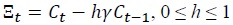E₀ denotes the conditional expectation at time t=0 and 0 < β < 1 denotes the time discount factor. In and γ are defined as the habit persistence parameter and the steady-state growth rate of global technology shock A_W,t (z_t=A_W,t/γA_W,t-1), respectively. τ>0 is the relative risk aversion coefficient and N_t is labor input.

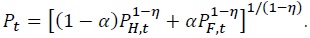
Suppose that 0 ≤ α < 1 is the import share and η>0 is the intratemporal substitution elasticity between domestic and foreign consumption goods. Then, the aggregate consumption index C_t is expressed as follows.

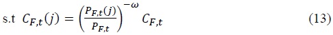
The aggregate expenditure is allocated by the households based on the demand function as follows.

P_H,t and P_F,t are home and foreign goods price indices, respectively. The consumption price index (CPI) is defined as The household budget constraint is as follows.

In equation (4), Q_t,t+1 and D_t+1 are the stochastic discount factor and the income from the asset portfolio, respectively, and E_t [Q_t,t+1 D_t+1] thus represent the amount of portfolio purchases at time t. T_t represents a lump-sum tax.

The household maximizes the intertemporal utility function under given budget constraints. Intertemporal consumption and optimal portfolio choices are expressed as follows.

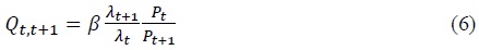
where 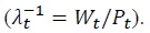λ_t is the marginal utility of income

The normal interest rate implies:

2) Domestic Products

Domestic producers are assumed to be monopolistic competition producers dependent on pricing of the Calvo type2 and have the following production function.

Here A_t is a domestic technology shock. The firm pursues profit maximization under the given demand function constraint as follows.

Here, MC_H,t=W_t/(A_W,t A_t P_H,t) and denotes the probability that the price adjustment of a specific firm is not allowed between periods N and t. G_H,t and asterisk (*) imply domestic government expenditure and the foreign country, respectively.3

3) Domestic Importer

It is assumed that short-term deviation from the PPP (purchasing power parity) occurs because the importer is in a monopolistic competition. The law of one price gap is defined as follows.

where e_t denotes the nominal exchange rate and ψ_F,t=1 when PPP holds. It is assumed that the importer, like domestic producers, is a Calvo type pricing setter4 and that domestic government cannot purchase foreign-produced goods. The importer maximizes the expected profit under given demand function constraints as follows.

4) Foreign Economy

Unlike Lubik and Schorfheide (2006), domestic and foreign economies are assumed to be different in terms of preference and risk aversion as well as pricing and monetary policy. That is, are assumed in the paper.5 Variables and parameters are marked with an asterisk in the equation representing the foreign economy.

The real exchange rate is defined as follows.

The foreign real exchange rate is equal to Conversely, domestic terms of trade q_t (=P_H,t/P_F,t) and foreign terms of trade differ by the law of one price gaps as follows:

Equation (15) can be derived by using the law of one price and when the path-through is perfect, the two trading conditions have the opposite relationship.

5) Risk Sharing, Market Liquidation, and Equilibrium

A complete international asset market without asset accumulation is assumed to avoid the complexity of the model, as in the case of Lubik and Schorfheide (2006). Since the complete international asset market assumption implies that the risk sharing between the two countries’ households is complete, the stochastic discount factor between the two countries in equilibrium equals:

The conditions for liquidation of the goods market are as follows.

2. Linear Equation System and Bayesian Estimation Technique

In the empirical analysis, the model equations are log-linearized around the steady state, for example, The logarithmic linear model consists of 22 equations of endogenous variables as shown in Appendix A and the following 5 equations of autoregressive exogenous shocks:

This linear equation system includes the Taylor-typed monetary policy rules of both countries in which the nominal interest rate responds to exchange rate fluctuations. As shown in (A11) and (A21), the shock on the monetary policy rule of each country is indicated by ε_R,t and ε_R*,t. The closed economy version of the model with α=0 is composed of (A1) domestic firm’s price setting, (A2) domestic habits, (A3) marginal utility of consumption, (A5) CPI definition, (A9) domestic goods market liquidation, (A11) monetary policy rule, (A22) Euler’s equation.

The logarithmic linear DSGE model can be represented by the following linear rational expectations model.

where m_t is the vector of model variables such as ε_t and υ_t are the vectors of exogenous shock and rational expectations error, respectively. θ is the structural parameter vector and the solution of equation (19) can be expressed as:

The measurement equation that connects model variables m_t and observation vectors y_t is as follows.

Here, y_t is composed of variables such as GDP growth, inflation, nominal interest rates, and won/dollar exchange rate changes. The matrix ∆(θ) is composed of 6 These equations are estimated by using the Bayesian estimation method.

A posterior density 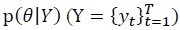is directly proportional to the likelihood function times a prior density p(θ) as follows.

where ∝ implies proportionality.

3. DSGE-VAR Estimation Method

To estimate the DSGE-VAR model, this study first considers the following reduced-form VAR model with n variables and q lags (An and Schorfheide, 2007).

Here, 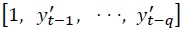x_t and Φ are defined to be the same as the explanatory variable vector and the coefficient matrix [Φ₀,Φ₁,⋅⋅⋅,Φ_q]', respectively and then VAR of equation (23) can be expressed as follows.

where Y and U are T×n matrices (T: sample size) of which each consists of rows and X is T×k (k=n×q+1) matrix composed of rows Estimating the DSGE model is about the same as estimating VARs with cross-equation constraints. The DSGE-VAR model is a way to systematically mitigate the cross-coefficient constraints imposed on the VAR by the DSGE model, which is an intermediate form of the VAR approximation of the DSGE model and the unconstrained VAR. The overall magnitude of these constraints is controlled by the hyperparameter μ which scales the covariance matrix of the prior. When μ approaches infinity, these restrictions are strictly applied, whereas when μ is zero, these restrictions are not considered at all when estimating VAR parameters.7 When is the expectation of the DSGE model, the autocovariance matrix is defined as

The VAR approximation of the DSGE model can be obtained from the following constraint function that links the parameters of the DSGE model with those of the VAR model.

The accuracy of this approximation depends on the number of lags q, and according to An and Schorfheide (2007), q=4 is sufficient to guarantee a precise approximation of the model.

To analyze impulse response, structural shock must first be identified from the reduced-form shock. In the VAR analysis, we generally first estimate the reduced-form VAR and then derive the structural parameters that represent the simultaneous relationships between endogenous variables through a variety of constraints, such as Cholesky decomposition, sign restrictions, and long-term restrictions. For instance, in the case of estimating the structural model Ay_t=A₀+A₁y_t-1+⋯+A_qy_t-q+ν_t using Cholesky decomposition, a parameter matrix A represents the direct causal relationship between the endogenous variables such as interest rates, exchange rates, and so on. Whereas, the reciprocal of A, A^-1, shows the overall effect including not only the direct causal relationship between the two variables but also the indirect causal relationship that occurs through other endogenous variables. In addition, the impulse response function of zero period indicates this overall effect.8 The reduced-form shock u_t in Eq. (23) can be expressed as a function of the structural shock ν_t (u_t=Σ_trΩν_t), of which the impulse response function of VAR is obtained as follows.

where Σ_tr is the Cholesky decomposition of Σ and Ω is the orthonormal matrix. Meanwhile, Del Negro and Schorfheide (2004) estimated the impulse response function of DSGE through QR factorization when Β(θ) is a simultaneous response of y_t to the shock ν_t in the DSGE model as follows.

where is a lower triangular matrix and Ω* (θ) is an orthonormal matrix.

To identify DSGE-VAR, Del Negro and Schorfheide (2004) and An and Schorfheide (2007) replaced the term Ω in Eq. (27) with Ω* (θ) in Eq. (28), keeping Σ_tr in Eq. (27) intact. If there is no misspecification in the model setup, a rotation matrix is selected so that the impulse responses of DSGE and DSGE-VAR match.

1)Since the several domestic studies have already examined the small open economy DSGE models, this study focuses on the asymmetric two-country open economy DSGE model. But the main impulse response results of the DSGE models for domestic inflation and the won/dollar exchange rate are similar without relation to model specification. Take look at Lubik and Schorfheide (2006) for the detailed contents of this model.

2)See (A1) in Appendix A. In equation (A1), implies marginal cost.

3)

4)See (A4) in Appendix A.

5)Take look at the Table 2 and Table 5. In two-country open economy models, it is generally known that heterogeneous models in which the response coefficients are not equal have better in-sample and out-of-sample performances than homogeneous models in which they are equal. For example, Molodtsova and Papell (2009), and Ince et al. (2016).

6)Take look at nkmp_mod.src in the GAUSS programs opened at the Schorfheide’s homepage.

7)Specifically, on a computer program, X’X in the DSGE-VAR is composed of X’X calculated from actual data and μT times X’X derived from the DSGE estimates (μ=∞,10,5,…,0.25). See p_varprior.g in the GAUSS programs. X’Y is also derived by the same method.

8)Please refer to Lee (2009, 2015) for details on how structural parameters and impulse response functions are derived and the economic implications they have.

IV. ESTIMATION RESULTS

Data used in estimations are real GDP, the consumer price index (CPI), the CD interest rate of Korea and the U.S., and the won/dollar exchange rate (Source: IFS). The equation for the short-term interest rate could be usually interpreted as a monetary policy reaction function. In previous many papers, a monetary policy reaction function often used the three-month interest rate (For example, Rigobon and Sack, 2003a; 2003b). Over the entire sample period, the correlation coefficient between rate of change of the call rate and rate of change of the CD rate is 0.943, with the two rates moving almost equally. The correlation coefficient between rate of change of the federal funds rate and rate of change of the U.S. CD rates is 0.854.9 The sample period is from the first quarter of 1990 to the first quarter of 2016 and the sample size is 105. For the real GDP, consumer price index, and won/dollar exchange rates due to the existence of a unit root, the rate of change multiplied by 100 (400 for consumer price index) is used and the sample size is reduced to 104. The level variable is used for interest rate data.

The DSGE and DSGE-VAR models are estimated for the sample period (1990:2-2016:1) and the period after the currency crisis and before the global financial crisis (1999:2-2007:1) to increase reliability of estimation results, as Korea experienced these two crises during the analysis period. Table 1 shows the prior distribution. It considers Lubik and Schorfheide (2006) and the domestic studies introduced in the literature review as reference. Beta and normal distribution are assumed for the case in which the parameter exists in a certain interval and is not limited to a specific interval, respectively. A gamma or inverse gamma distribution is given for the case in which the parameter has a positive value. Unlike Lubik and Schorfheide (2006), in this study, which assumes that the real sector of the both countries is not symmetric, the parameters such as are additionally estimated.

Table 2 shows the posterior distribution of the DSGE-VAR (μ=∞) parameter estimates over the period in which the two economies were relatively stable, that is, the period from the post-currency crisis to the pre-global financial crisis (1999:2-2007:1). The posterior distribution is simulated using the Metropolis-Hasting algorithm. Simulation and burn-in sizes are 1,000,000 and 200,000, respectively. While the estimates of τ and h are like those of τ* and h*, the estimates of are relatively different from those of But these estimates are also inside the 90% confidence interval of the other country estimate, respectively. The estimate of the parameter ψ₃ revealing the response of the domestic interest rate to the won/dollar exchange rate is 0.102 and statistically significant at the 5% level, while the estimate of the parameter revealing the response of the U.S. interest rate is close to zero.

Table 3 shows the marginal data density for DSGE, DSGE-VAR (μ) (μ= ∞, 10, 5, 2), and Bayesian VAR during the same period.10 In the Bayesian framework, the marginal data density of the DSGE-VAR (μ=10) is the best at -337.331 and is not significantly different from that of DSGE-VAR (μ=∞). The marginal data density of the DSGE model is defined as P(Y)=∫L (θ|Y)p(θ)dθ. The marginal data density is simply the integral of the likelihood taken according to the prior distribution. In other words, it is the weighted average of the likelihood where the weights are given by the prior. Table 3 displays that the marginal data density has an inversed U-shaped pattern as in Del Negro and Schorfheide (2006). The marginal data density criterion considers the estimation fit and the complexity of the model. Table 4 presents the in-sample RMSE. The RMSE of the Bayesian VAR model is less than that of the DSGE model.

Figure 1 shows responses of domestic macroeconomic variables to domestic interest rate hike shocks of one standard deviation size, derived from results of the estimation of DSGE-VAR (μ=∞) over the period from the post-currency crisis to the pre-global financial crisis (1999:2-2007:1). Since the main impulse response results of the DSGE and DSGE-VAR (μ) (μ= ∞, 10, 5, 2) are similar, only the case of μ= ∞ is reported in this study.11 The solid line and the dotted line represent the average response and the 90% confidence interval of DSGE-VAR (μ=∞), respectively, and the dashed line stands for the average response of DSGE. The average responses of DSGE-VAR (μ=∞) almost coincide with those of DSGE. As in the case of DSGE estimation results of other domestic studies, the positive interest rate shock lowers domestic GDP and prices, and raises the value of the won.12

Table 5 shows the posterior distribution of DSGE-VAR (μ=1) parameter estimates for the entire sample period (1990:2-2016:1). As presented in Table 6, according to the marginal data density standard, DSGE-VAR (μ=1) is better than DSGE or other DSGE-VAR. Hence, this study reports only the case of DSGE-VAR (μ=1). Compared to Table 2, the estimates of revealing price rigidity are not significantly different. This is because the sample period includes pre-currency crisis and post-global financial crisis periods. In the case of Korea after the global financial crisis, unlike the zero interest rate period in the U.S., which is accompanied by non-traditional monetary policies such as quantitative easing or credit easing policies and interest on required reserve balances and excess balances, the standard for distinguishing low interest rate and high interest rate period is not clear. For major developed economies using zero interest rates policies, quantitative easing or credit easing policies are used to stimulate the economy because of zero lower bound restrictions where the nominal interest rate cannot fall below zero. But we need not use quantitative easing policies in situations where we can afford to cut interest rates. Also, although the revised Bank of Korea law stipulates interest can be paid for reserve balances, it does not currently pay actual interest, as are the case with the U.S. and the ECB. Owing to these changes and differences in monetary policies, the correlation between the federal funds rate and the U.S. CD interest rate seems to be smaller than the correlation between the call rate and the CD interest rate and the estimation results of all models are better, when using the CD interest rates of both countries. As the sample period is moved from the past to the present, estimates of become less. In contrast to Table 2, while the estimate of τ* varies significantly, estimates of are not significantly different from those of 13 The estimate of the parameter revealing the response of the domestic interest rate to the won/dollar exchange rate is 0.070 and statistically significant, but less than that of Table 2. Meanwhile, the response of the U.S. interest rate is close to zero.

Table 6 shows the marginal data densities of DSGE-VAR (μ=∞, 5, 1, 0.75, 0.5, 0.25) and Bayesian VAR over the whole sample period. The marginal data density of the DSGE-VAR (μ=1) is the best at -1291.267. In Table 6, the marginal data density has a reversed U-shaped pattern. It implies that the DSGE model is misspecified. Table 7 presents the in-sample RMSE. The RMSE of the Bayesian VAR is less than that of DSGE-VAR as well as DSGE. In the case of the reduced-form VAR with block-exogeneity (Lastrapes, 2005), the in-sample RMSE is much less than those of these models, although it is not shown in the table. The in-sample RMSEs for the seven variables in order of Table 7 are 0.494, 1.843, 0.344, 0.950, 1.962, 0.915, and 4.206, respectively. In non-Bayesian estimation methods, parameters are treated as unknown constants. But the Bayesian estimation method considers parameters as probability variables. So the study does not report this result in Table 7.

Figure 2 describes the responses of the domestic macroeconomic variables to positive domestic interest rate shocks corresponding to one unit of standard deviation based on the estimation results of the DSGE-VAR (μ=∞) over the sample period (1990:2-2016:1). The solid line and the dotted line reveal the average response and the 90% confidence interval of DSGE-VAR (μ=∞), respectively, and the dotted line represents the average response of DSGE. In contrast with Figure 1, the average response of DSGE-VAR (μ=∞) do not necessarily match that of DSGE depending on variables. Figure 3 depicts the response of the DSGE-VAR (μ=1). Unlike Figure 2 as well as Figure 1, average impulse responses of the DSGE-VAR (μ=1) and the DSGE do not significantly coincide. As we have observed in comparisons of marginal data density and the in-sample RMSE, the DSGE-VAR (μ=1) is superior to the DSGE for the whole sample period. However, like the case of other DSGE models, a positive interest rate shock lowers domestic GDP and prices, and increases the won value.14 This result is also true if using other prior distributions, for example, assuming that the prior distribution of follows a uniform distribution instead of the beta distribution, or that the parameters such as are equal to 0. The same is true if using demeaned data.

Figure 4 shows the response of domestic macroeconomic variables to domestic interest rate hike shocks, equivalent to one unit of standard deviation, using the Bayesian VAR (4) model. Unlike the DSGE and DSGE-VAR models, positive interest rate shocks lower GDP in the early stages, while raising prices and lowering the value of the won. The same conclusions are reached in the case of a simple reduced-form VAR using Cholesky decomposition as well as in the case of a VAR assuming block-exogeneity and a VAR using sign restrictions.15

In this study, DSGE, DSGE-VAR, and Bayesian VAR are estimated by focusing on the Bayesian estimation technique and the estimation results reveal that the DSGE-VAR is relatively superior in the marginal data density criterion. However, when the estimation results of the DSGE-VAR and traditional VAR models are measured with the in-sample RMSE standard, the latter is better, especially for the won/dollar exchange rate.

9)The DSGE model is estimated relatively well regardless of the period when the CD interest rates of both countries are used, whereas the DSGE model is not well estimated by the period when using the call rate and the federal funds rate.

10)The study describes the estimation results for the Bayesian VAR using the number of lags 4 and the Minnesota prior with λ₁=1, λ₂=4, λ₃=1, λ₄=1, and λ₅=1. See Del Negro and Schorfheide (2011) for the Minnesota prior and the marginal data density criterion. Take a look at var_margpm.g in the GAUSS programs and Del Negro and Schorfheide (2006) for the optimal choice of μ.

11)This result may be natural, because a bigger weight (μT) is given to X’X and X’Y derived from the DSGE estimation results. But when μ is smaller than 0.25, the converged estimation results cannot be obtained. See note 7.

12)See Figure A1 in Appendix for the responses of each variable to total seven shocks. In the figure, A→B means the dynamic response of the variable B to the shock of the variable A.

13)

14)See Figure A2 in Appendix for the responses of each variable to total seven shocks.

15)Figure A3 in Appendix displays the impulse response of VAR with block-exogeneity.

V. IMPLICATION

From the impulse response analysis, a positive domestic interest rate shock lowers domestic inflation and raises the won value in the case of DSGE and DSGE-VAR models. Conversely, the reverse is the case in the unrestricted VAR model. According to the in-sample RMSE standard, the unrestricted VAR models have better explanatory power on major economic variables than the DSGE and DSGE-VAR models, especially for the won/dollar exchange rate. Results reveal that the (New) Keynesian structural approach, suggesting that the expansionary monetary policy leads to income growth and inflation through the interest rate path, may not be suitable to Korea because its dependence on foreign trade and openness of stock markets is considerably significant. Stronger cross-equation restrictions of the DSGE model leading to a lower explanatory power of model may imply that the complicated Korean economic reality may be explained with a New Classical approach or other approaches. For a recent empirical example, Engel et al. (2017) used data of U.S. dollar exchange rates and money market rates from January 1999 to December 2015 in eight countries (Canada, Denmark, Euro area, Japan, Norway, Switzerland, Sweden, and UK) and tested whether the uncovered interest parity (UIP) held. They found that, unlike the existing UIP estimates, the parameter estimates for interest rate differentials were negative only in four of the eight countries, and in any case these estimates were not significantly different from zero. Furthermore, the UIP puzzle did not hold for these data because the null hypothesis for UIP that the coefficient was equal to 1 for all exchange rates was not rejected.16

A domestic interest rate hike raises the value of domestic currency according to the traditional Keynesian theory, assuming price rigidity, while lowers domestic currency value according to the Chicago school theory that assumes price flexibility. However, in this study, impulse response results of DSGE and DSGE-VAR are not reversed even when assuming that , indicating price rigidity, are equal to 0. This indicates that other paths or variables, rather than price flexibility assumption, may influence a causal relationship or correlation between these variables. For example, in Korea, where the stock market is fully open, a domestic interest rate hike will lead to a decline in share prices (and GDP), and a decline in share prices (and GDP) will lead to a rise of the won/dollar exchange rate due to capital outflow, which causes inflation. Korea’s stock and bond markets have already been fully opened to foreigners since 1998, but unlike the stock market, the share of Korean bonds held by foreign investors was only 0.5 percent before 2007. Accordingly, the domestic bond market has not been highly interconnected with the domestic and overseas stock and foreign exchange markets unlike the domestic stock market. The average annual market value of foreign-owned stock stood at 216.2 trillion won in the 20 years from 1996 to 2015, while the average annual foreign-invested bond investment was 32.6 trillion won, accounting for only 16.0 percent of the market value of foreign-owned stock. Thus, in Korea, foreign capital has come through the stock market path, not through the bond market path.

In case of the U.S., a so-called ‘price puzzle’ problem is solved by additionally including the sensitive commodity price in VAR models. But in case of Korea, this phenomenon is not disappeared, even though the other several prices are considered together in VAR models. It seems to happen, because domestic inflation is largely influenced by won/dollar exchange rates and its dependence on foreign trade and openness of stock market is considerable. The correlation coefficient estimates in Table 8 show this possibility. When the currency crisis and global financial crisis periods are excluded, a positive correlation between ΔKRCPI_t and ΔKRINT_t-k is bigger. If the GDP deflator is used instead of the consumer price index, a correlation between domestic inflation and interest rates is reduced. But the main results is not changed. The same results are also obtained from the OECD data. Table 8 also demonstrates that the rise in domestic inflation is more closely related to the rise in the won/dollar exchange rate and U.S. inflation than to decline in domestic interest rates. The impulse response analysis in the VAR model displays this result (e.g. Lee, 2015). In addition, if the interest rate and import increase because of ongoing boom, the current account balance will deteriorate and the won/dollar exchange rate will rise. The depreciation of the won against the U.S. dollar may possibly lead to a rise in domestic inflation. In relation to the cause of the inconsistency of the impulse responses between DSGE or DSGE-VAR, and VAR models, a more in-depth study on if these differences are caused by model misspecification or omitted variable bias related to the trade sector or capital market is necessary.

This study objectively examines effects of Korean monetary policy on income, prices, and won/dollar exchange rates using DSGE, DSGE-VAR, and VAR models with continuity in relation to the cross-equation restrictions. Empirical results achieved through this complex process are expected to facilitate implementation of monetary and foreign exchange policies in the direction of maximizing the welfare of the national economy without being disturbed by special interest groups in the future.

16)According to Engel et al. (2017), when U.S. inflation was added in the UIP regression of the change in the exchange rate on the interest rate differential, the inflation variable was highly significant but the interest rate differential was not. Their estimation results are similar to those of Molodtsova and Papell (2009), and Ince et al. (2016). Since 1990, many central banks have been adopting inflation targeting as an operating system of monetary policy. It was also shown that when survey data were used as the inflation variable, estimates of parameters for the interest rate differential all had a positive value and that for the Euro zone and Sweden there was also a statistical significance. Engel et al. (2017) argued that the movement of interest rates reflected not only the direction of monetary policy but also the perceptions of the relative liquidity of short-term financial assets. In other words, if the home interest rate rises due to monetary tightening, the value of the home currency increases, while the value of the home currency declines as the home interest rate rises because home interest bearing assets have low liquidity return.

VI. CONCLUSIONS

This study analyzes the effects of domestic monetary policy on national income, prices, and won/dollar exchange rates using DSGE, DSGE-VAR, and VAR models based on the open macroeconomic theory. In the empirical analysis, quarterly real GDP, CPI, CD interest rate data of Korea and the U.S. as well as won/dollar exchange rate data from 1990 to the present are used.

First, the empirical analysis for the period from post-currency crisis to pre-global financial crisis (1999:2-2007:1) reveals that the DSGE-VAR (μ=10) is slightly better than the DSGE and the other DSGE-VAR in the marginal data density standard. Conversely, the in-sample RMSE is the lowest in the Bayesian VAR. In the case of μ=∞, the impulse responses of DSGE and DSGE-VAR relatively come into line.

For the whole period (1990:2-2016:1), the DSGE model and the DSGE-VAR model are estimated using the same prior distribution for the period from post-currency crisis to pre-global financial crisis. In this case, DSGE-VAR (μ=1) is superior to DSGE and other DSGE-VARs. Marginal data density is inversely U-shaped according to the value of μ, and the largest is the case of μ=1.17 In the case of μ=∞, the impulse response results of DSGE and DSGE-VAR are less similar, in contrast with those for the stable period. For this period, the in-sample RMSE of Bayesian VAR is lower than that of the structural models. In addition, the simple reduced-form VAR model with block-exogeneity has the lowest in-sample RMSE.

According to the impulse response analysis over the sample period, the domestic interest rate hike shock raises won value in the case of the DSGE model and the DSGE-VAR model. Empirical results are identical in the period from the post-currency crisis to the pre-global financial crisis and not also influenced by the other assumptions of prior distributions and parameter restrictions. In the case of a Bayesian VAR or a simple reduced-form VAR, it lowers the won value. According to the RMSE standard, the in-sample RMSE of the DSGE models is larger than that of the unrestricted VAR model for GDP growth and inflation. The parameter estimation results also reveal that in Korea, the movement of the won/dollar exchange rate affects the domestic interest rate, unlike in the U.S.

In relation to the cause of inconsistent impulse response results between structural and reduced-form models, it is necessary to investigate what kinds of model misspecification or omitted variable bias these differences come from and if these problems are closely related to trade sectors or capital markets.18

17)Del Negro and Schorfheide (2006) interpreted a reversed U-shaped pattern as evidence of misspecification. Stiglitz (2017) made the following arguments in the conclusion of his paper. “~ Defenders of DSGE models counter that other models did little better than the DSGE models. That is not correct. ~”

18)Korea experienced changes in the exchange rate system and the monetary policy as well as the currency and the global financial crises during the entire sample period. It suggests that it is necessary to consider structural breaks in the economy and regime shifts in policy. From a methodological point of view, a DSGE (or VAR) with constant parameters can be extended to a Markov-switching DSGE (or VAR), even though it is very difficult in estimation. The latter may have better performance than the former.

Appendix A.

References

- Adolfson, M., Lassén, S., Lindé, J. and M. Villani. 2004. Bayesian Estimation of an Open Economy DSGE Model with Incomplete Pass-Through. Sveriges Riksbank. Manuscript.
- Ambler, S., Dib, A. and N. Rebei. 2004. Optimal Taylor Rules in an Estimated Model of a Small Open Economy. Bank of Canada. Staff Working Paper, no. 2004-36.
-
An, S. and F. Schorfheide. 2007. “Bayesian Analysis of DSGE Models,”
Econometric Reviews , vol. 26, no. 2-4, pp. 113-172.
Bergin, P. R. 2003. “Putting the ‘New Open Economy Macroeconomics’ to a Test,”
Journal of International Economics , vol. 60, no. 1, pp. 3-34.
Bergin, P. R. 2006. “How Well Can the New Open Economy Macroeconomics Explain the Exchange Rate and the Current Account?,”
Journal of International Money and Finance , vol. 25, no. 5, pp. 675-701.
Clarida, R. and J. Gali. 1994. “Sources of Real Exchange Rate Fluctuations: How Important Are Nominal Shocks?,”
Carnegie-Rochester Conference Series on Public Policy , vol. 41, pp. 1-56.
Clarida, R., Gali, J. and M. Gertler. 1999. “The Science of Monetary Policy: A New Keynesian Perspective,”
Journal of Economic Literature , vol. 37, no. 4, pp. 1661-1707.
- Del Negro, M. 2003. Fear of Floating: A Structural Estimation of Monetary Policy in Mexico. Federal Reserve Bank of Atlanta. Manuscript.
Del Negro, M. and F. Schorfheide. 2004. “Priors from General Equilibrium Models for VARs,”
International Economic Review , vol. 45, no. 2, pp. 643-673.
Del Negro, M. and F. Schorfheide. 2006. “How Good Is What You’ve Got? DOSE-VAR as a Toolkit for Evaluating DSGE Models,”
Federal Reserve Bank of Atlanta Economic Review , vol. 91, no. 2, pp. 21-37. -
Del Negro, M., Schorfheide, F., Smets, F. and R. Wouters. 2007. “On the Fit of New-Keynesian Models,”
Journal of Business and Economic Statistics , vol. 25, no. 2, pp. 123-143.
Del Negro, M. and F. Schorfheide. 2011. Bayesian Macroeconomics. In Geweke, J., Koop, G. and H. van Dijk. (eds.)
The Oxford Handbook of Bayesian Econometrics . Oxford: Oxford University Press. pp. 293-389. - Dib, A. 2003. Monetary Policy in Estimated Models of Small Open and Closed Economies. Bank of Canada. Working Paper, no. 2003-27.
- Engel, C., Lee, D., Liu, C., Liu, C. and S. Wu. 2017. The Uncovered Interest Parity Puzzle, Exchange Rate Forecasting, and Taylor Rules. NBER Working Paper, no. 24059.
Farrant, K. and G. Peersman. 2006. “Is the Exchange Rate a Shock Absorber or a Source of Shocks? New Empirical Evidence,”
Journal of Money, Credit, and Banking , vol. 38, no. 4, pp. 939-961.
Gali, J. and T. Monacelli. 2005. “Monetary Policy and Exchange Rate Volatility in a Small Open Economy,”
Review of Economic Studies , vol. 72, no. 3, pp. 707-734.
Ince, O., Molodtsova, T. and D. H. Papell. 2016. “Taylor Rule Deviations and Out-of-Sample Exchange Rate Predictability,”
Journal of International Money and Finance , vol. 69, pp. 22-44.
- Justiniano, A. and B. Preston. 2004. Small Open Economy DSGE Models: Specification, Estimation, and Model Fit. Columbia University. Manuscript.
Kang, H-D. and D-H. Pyeon. 2009. “Development Status of DSGE Model for the Economic Outlook of the Bank of Korea (BOKDPM),”
Monthly Statistical Bulletin , vol. 63, no. 1, pp. 57-86. Bank of Korea. (in Korean) -
Kang, H-K., Park, Y. S. and J. Choi. 2014. “Recent Developments and Challenges in DSGE Modeling at Central Banks: A Survey,”
Economic Analysis , vol. 20, no. 1, pp. 94-144. Bank of Korea. (in Korean) -
Kim, K-H. 2011. “Household Credit Channel and Exchange Rate Channel in the Transmission Mechanism of Monetary Policy in Korea: Analysis Based on a Small Open Economy DSGE Model,”
Journal of Korean Economic Analysis , vol. 17, no. 2, pp. 127-166. Korea Institute of Finance. (in Korean) -
Lastrapes, W. D. 2005. “Estimating and Identifying Vector Autoregressions under Diagonality and Block Exogeneity Restrictions,”
Economics Letters , vol. 87, no. 1, pp. 75-81.
- Lee, H-G. 2013. An Analysis of Characteristics and Drivers of Economic Fluctuations in Korea Using the KDI-DSGE Model. Research Materials, no. 2013-01. Korea Development Institute. (in Korean)
Lee, K. Y. 2009. “Exchange Rate Pass-Through on Import and Domestic Prices,”
Korean Journal of Economic Studies , vol. 57, no. 4, pp. 39-71. (in Korean) -
Lee, K. Y. 2015. “The Dynamic Causal Relationship between Interest Rates, Exchange Rates and Prices,”
Journal of Money & Finance , vol. 29, no. 4, pp. 129-159. (in Korean) - Leeper, E. and C. Sims. 1994. Toward a Modern Macroeconomic Model Usable for Policy Analysis. NBER Working Paper, no. 4761.
- Leigh, D. and T. Lubik. 2005. Monetary Policy and Imperfect Pass-Through: A Tale of Two Countries. Johns Hopkins University. Manuscript.
Liu, P. and K. Theodoridis. 2012. “DSGE Model Restrictions for Structural VAR Identification,”
International Journal of Central Banking , vol. 8, no. 4, pp. 61-95. -
Lubik, T. A. and F. Schorfheide. 2006. A Bayesian Look at New Open Economy Macroeconomics. In Gertler, M. and K. Rogoff. (eds.)
NBER Macroeconomics Annual 2005 , vol. 20, pp. 313-366. Cambridge: MIT Press. -
Lubik, T. A. and F. Schorfheide. 2007. “Do Central Banks Respond to Exchange Rate Movements? A Structural Investigation,”
Journal of Monetary Economics , vol. 54, no. 4, pp. 1069-1087.
Molodtsova, T. and D. H. Papell. 2009. “Out-of-Sample Exchange Rate Predictability with Taylor Rule Fundamentals,”
Journal of International Economics , vol. 77, no. 2, pp. 167-180.
Obstfeld, M. and K. Rogoff. 1995. “Exchange Rate Dynamics Redux,”
Journal of Political Economy , vol. 103, no. 3, pp. 624-660.
- Park, M-H. 2013. Macroeconomic Impact Analysis of Monetary Policy Using a Small Open Economy DSGE Model. National Pension Research Institute. Working Paper, no. 2013-01. (in Korean)
Rigobon, R. and B. Sack. 2003a. “Measuring the Reaction of Monetary Policy to the Stock Market,”
Quarterly Journal of Economics , vol. 118, no. 2, pp. 639-669.
- Rigobon, R. and B. Sack. 2003b. Spillovers across U.S. Financial Markets. NBER Working Paper, no. 9640.
Schorfheide, F. 2000. “Loss Function-Based Evaluation of DSGE Models,”
Journal of Applied Econometrics , vol. 15, no. 6, pp. 645-670.
Smets, F. and R. Wouters. 2003. “An Estimated Dynamic Stochastic General Equilibrium Model of Euro Area,”
Journal of the European Association , vol. 1, no. 5, pp. 1123-1175.
- Stiglitz, J. E. 2017. Where Modern Macroeconomics Went Wrong. NBER Working Paper, no. 23795.
- Warne, A., Coenen, G. and K. Christoffel. 2013. Predictive Likelihood Comparisons with DSGE and DSGE-VAR Models. European Central Bank. Working Paper, no. 1536.