Electromagnetic Devices with Moving Parts—Simulation with FEM/BEM Coupling

Abstract

The numerical analysis of electromagnetic devices by means of finite element methods (FEM) is often hindered by the need to incorporate the surrounding domain. The discretisation of the air may become complex and has to be truncated by artificial boundaries incurring a modelling error. Even more problematic are moving parts that require tedious re-meshing and mapping techniques. In this work, we tackle these problems by using the boundary element method (BEM) in conjunction with FEM. Whereas the solid parts of the electrical device are discretised by FEM, which can easily account for material non-linearities, the surrounding domain is represented by BEM, which requires only a surface discretisation. This approach completely avoids an air mesh and its re-meshing during the simulation with moving or deforming parts. Our approach is robust, shows optimal complexity, and provides an accurate calculation of electromagnetic forces that are required to study the mechanical behaviour of the device.

1. Introduction

The digital development of electromagnetic devices usually requires a coupled multi-physical approach to achieve a sufficiently accurate prediction of electrical and mechanical properties. Examples are electric motors, actuators or eddy-current brakes and also processes such as magnetic metal forming. Their functionality is determined by the effect of electromagnetic forces induced by permanent magnets or AC coils.

Conventional simulation methods are based on the finite element method (FEM) and rely on the domain discretisation of both the solid parts and the surrounding air or protective gas environment; however, this has some significant drawbacks for the design engineer: the volume of the surrounding domain is usually not covered by the computer-aided design (CAD) model and its domain needs to be discretised and artificially truncated. This potentially introduces non-physical boundary conditions. Moreover, if individual parts move against each other or are subject to large deformations, frequent and tedious re-meshing of the surrounding domain is required, which leads to additional modelling and computational effort.

As an alternative to FEM, the boundary element method (BEM) [1] can be used to simulate the surrounding domain. A surface discretisation is sufficient to incorporate the complete exterior domain fulfilling the decay conditions exactly. This means that moving components can be handled in an intriguingly simple fashion by completely avoiding air meshes and re-meshing.

The advantage of coupling both methods is well known and has been addressed by [2,3] at an early stage. Different approaches of FEM/BEM coupling schemes for eddy-current problems have been proposed e.g., in [4,5]. In this work, we present a symmetric coupling scheme based on [6]. It utilises the particular advantages of the involved numerical methods and provides the application engineer with an easy-to-use, versatile, and accurate simulation tool.

This paper is organised as follows: After introducing the continuous formulation in Section 2, the spatial and temporal discretisation as well as the Newton method are briefly presented in Section 3. In Section 4 we explain how a robust and optimally scalable implementation has been achieved by using special solution and preconditioning strategies as well as acceleration techniques for the solution of the system of equations. As a crucial post-processing step, the force calculation is explained in Section 5. Finally, the accuracy of the proposed methodology is demonstrated in Section 6 using established benchmark problems and its applicability is shown by means of practical examples.

2. Continuous Formulation

2.1. Eddy-Current Model

The underlying problem considered in this work is the eddy-current model that is obtained from Maxwell’s equations by neglecting the displacement current $\mathit{D}$. The remaining set of equations reads [7]

$$\begin{array}{cc}\hfill \mathbf{curl}\mathit{H}& =\mathit{J}\hfill \end{array}$$

(1)

$$\begin{array}{cc}\hfill \mathbf{curl}\mathit{E}& =-\frac{\partial \mathit{B}}{\partial t}\hfill \end{array}$$

(2)

$$\begin{array}{cc}\hfill div\mathit{B}& =0,\hfill \end{array}$$

(3)

which are, in order, Ampère’s law, Faraday’s law, and Gauß’s law for magnetism. The involved fields are the magnetic field strength $\mathit{H}$, the current density $\mathit{J}$, the electric field $\mathit{E}$, and the magnetic flux intensity $\mathit{B}$. These equations are supplemented by the material laws

$$\begin{array}{cc}\hfill \mathit{B}& =\mu \left(\mathit{H}+\mathit{M}\right)\hfill \end{array}$$

(4)

$$\begin{array}{cc}\hfill \mathit{J}& ={\mathit{J}}_s+\sigma \mathit{E}\hfill \end{array}$$

(5)

with the magnetic permeability $\mu$, the electric conductivity $\sigma$, a given magnetisation $\mathit{M}$, and the applied source current density ${\mathit{J}}_s$. Note that relation between the $\mathit{H}$- and $\mathit{B}$-fields can be non-linear, in which case, the permeability $\mu$ depends on the field strength. Furthermore, the inverse of $\mu$ is denoted by the reluctivity $\nu$ and it is customary to use the decompositions

$$\mu ={\mu }_0{\mu }_r\mathrm{and}\nu ={\nu }_0{\nu }_r=\frac{1}{{\mu }_0}{\nu }_r$$

(6)

with the permeability of free space ${\mu }_0=4\pi ·{10}^{-7}\mathrm{H}/m$ and the dimensionless scalars ${\mu }_r$ and ${\nu }_r=\frac{1}{{\mu }_r}$. For air and vacuum we assume ${\mu }_r={\nu }_r=1$. Furthermore, expression (5) contains the term ${\mathit{J}}_e=\sigma \mathit{E}$, which represents Ohm’s law and yields the induced or eddy currents ${\mathit{J}}_e$. Since ${\mathit{J}}_s$ and $\mathit{M}$ are prescribed known quantities, the above set of equations can be expressed by only one vector field. Here, we make use of the $\mathit{A}$-based formulation in which an artificial vector potential $\mathit{A}$ is introduced such that

$$\mathit{B}=\mathbf{curl}\mathit{A}$$

(7)

and, therefore, Equation (3) is automatically fulfilled. Plugging all equations together and making use of a temporal gauging [7], we obtain the second-order partial differential equation

$$\sigma \frac{\partial \mathit{A}}{\partial t}+\mathbf{curl}\left[\nu (\mathbf{curl}\mathit{A})\mathbf{curl}\mathit{A}-\mathit{M}\right]={\mathit{J}}_s.$$

(8)

The above equations are valid in the entire space ${\mathbb{R}}^3$ and across any material interface the following transmission conditions hold

$$〚\mathit{H}\times \mathit{n}〛=\mathit{0}\mathrm{and}〚\mathit{A}\times \mathit{n}〛=\mathit{0},$$

(9)

where $\mathit{n}$ is a unit vector normal to the considered surface. In these conditions, we assume the absence of surface currents and similar fields. Note, that in conducting regions ($\sigma >0$) the electric field is given by

$$\mathit{E}=-\frac{\partial }{\partial t}\mathit{A},$$

(10)

whereas in non-conducting regions ($\sigma =0$) it is not uniquely defined [7]. For later purposes, we also define the magnetostatic energy as

$$w(\mathit{B})={\int }_0^B\mathit{H}(\beta )\mathrm{d}\beta ,$$

(11)

where we assume that the material is always isotropic, that is $\mathit{B}$ and $\mathit{H}$ are always co-linear. Moreover, B and H are the magnitudes of the $\mathit{B}$- and $\mathit{H}$-fields, respectively.

2.2. Weak Form

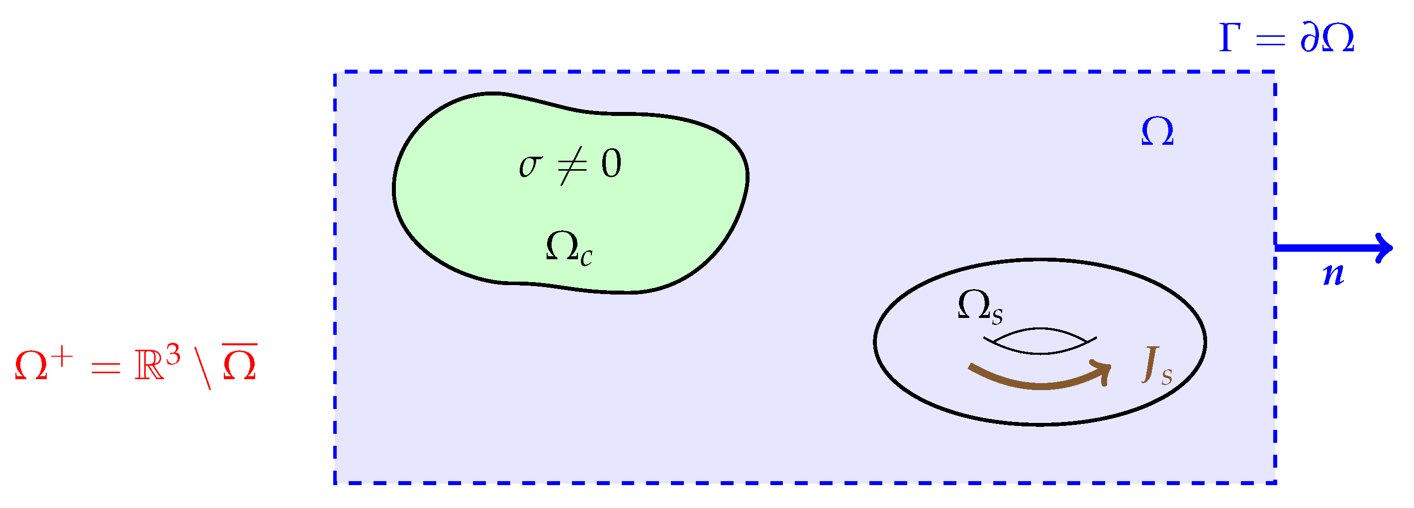
In order to develop a finite and boundary element discretisation of the considered eddy-current problem, we first establish a weak form. To this end, let $\mathsf{\Omega }$ denote an embedding domain, which can be multiply connected and consist of disconnected subdomains. For simplicity, in Figure 1, a rectangular domain is depicted, which encompasses the regions with applied source currents and the regions with conducting materials. Let ${\mathit{L}}_2(\mathsf{\Omega })$ denote the space of vector-valued functions $\mathit{f}$ whose components are square-integrable in the domain $\mathsf{\Omega }$ [8]. With this function space, we define

$${\mathit{X}}_{\mathsf{\Omega }}=\mathit{H}(\mathbf{curl},\mathsf{\Omega })=\left\{\mathit{f}\in {\mathit{L}}_2(\mathsf{\Omega }): \mathbf{curl}\mathit{f}\in {\mathit{L}}_2(\mathsf{\Omega })\right\}.$$

(12)

For the sake of readability, we abbreviate with ${\partial }_t(·)$ the time derivative and denote the ${\mathit{L}}_2$-inner product between two vector-valued function $\mathit{f}$ and $\mathit{g}$ as

$${\left(\mathit{f},\mathit{g}\right)}_{\mathsf{\Omega }}={\int }_{\mathsf{\Omega }}\mathit{f}·\mathit{g}\mathrm{d}\mathsf{\Omega }.$$

(13)

Using a weighted-residual method with test function ${\mathit{A}}^{\prime }\in {\mathit{X}}_{\mathsf{\Omega }}$, we obtain via integration by parts

$$\begin{array}{cc}\hfill 0& ={\left(\sigma {\partial }_t\mathit{A}+\mathbf{curl}\left[\nu \mathbf{curl}\mathit{A}-\mathit{M}\right]-{\mathit{J}}_s,{\mathit{A}}^{\prime }\right)}_{\mathsf{\Omega }}\hfill \\ \hfill & ={\left(\sigma {\partial }_t\mathit{A},{\mathit{A}}^{\prime }\right)}_{\mathsf{\Omega }}+{\left(\nu \mathbf{curl}\mathit{A},\mathbf{curl}{\mathit{A}}^{\prime }\right)}_{\mathsf{\Omega }}+{\langle {\mathit{H}}_{\times }^{-},{\gamma }_D^{-}{\mathit{A}}^{\prime }\rangle }_{\mathsf{\Gamma }}-{\left(\mathit{M},\mathbf{curl}{\mathit{A}}^{\prime }\right)}_{\mathsf{\Omega }}-{\left({\mathit{J}}_s,{\mathit{A}}^{\prime }\right)}_{\mathsf{\Omega }}.\hfill \end{array}$$

(14)

In the last expression, so-called trace operators are used, which are defined as

$$\begin{array}{cc}\hfill {\gamma }_D^{\pm }\mathit{A}& {=\mathit{n}\times \mathit{A}|}_{\mathsf{\Gamma }}^{\pm }\times \mathit{n}\hfill \end{array}$$

(15)

$$\begin{array}{cc}\hfill {\mathit{H}}_{\times }^{\pm }& =\left(\nu \mathbf{curl}\mathit{A}-\mathit{M}\right){{|}_{\mathsf{\Gamma }}^{\pm }\times \mathit{n}=\nu {\gamma }_N^{\pm }\mathit{A}-\mathit{M}|}_{\mathsf{\Gamma }}^{\pm }\times \mathit{n},\hfill \end{array}$$

(16)

where the function limits to the boundary are

$${\mathit{f}|}_{\mathsf{\Gamma }}^{\pm }(x)=\underset{\epsilon \to 0}{lim}\mathit{f}(x\pm \epsilon \mathit{n})x\in \mathsf{\Gamma }.$$

(17)

At last, there is the duality paring ${\langle ·,·\rangle }_{\mathsf{\Gamma }}$, which reads

$${\langle \mathit{f},\mathit{g}\rangle }_{\mathsf{\Gamma }}={\int }_{\mathsf{\Gamma }}\mathit{f}·\mathit{g}\mathsf{\Gamma },$$

(18)

where the function regularities and thus corresponding spaces for each slot are detailed in [6]. For further conciseness, we re-write Equation (14) as

$$m({\partial }_t\mathit{A},{\mathit{A}}^{\prime })+a_{\nu }(\mathit{A},{\mathit{A}}^{\prime })+{\langle {\mathit{H}}_{\times }^{-},{\gamma }_D^{-}{\mathit{A}}^{-}\rangle }_{\mathsf{\Gamma }}=\ell ({\mathit{A}}^{\prime })$$

(19)

with the abbreviations

$$\begin{array}{cc}\hfill m({\partial }_t\mathit{A},{\mathit{A}}^{\prime })& ={\left(\sigma {\partial }_t\mathit{A},{\mathit{A}}^{\prime }\right)}_{\mathsf{\Omega }}={\left(\sigma {\partial }_t\mathit{A},{\mathit{A}}^{\prime }\right)}_{{\mathsf{\Omega }}_c}\hfill \end{array}$$

(20)

$$\begin{array}{cc}\hfill a_{\nu }(\mathit{A},{\mathit{A}}^{\prime })& ={\left(\nu \mathbf{curl}\mathit{A},\mathbf{curl}{\mathit{A}}^{\prime }\right)}_{\mathsf{\Omega }}\hfill \end{array}$$

(21)

$$\begin{array}{cc}\hfill \ell ({\mathit{A}}^{\prime })& ={\ell }_J({\mathit{A}}^{\prime })+{\ell }_M({\mathit{A}}^{\prime })={\left(\mathit{J},{\mathit{A}}^{\prime }\right)}_{{\mathsf{\Omega }}_s}+{\left(\mathit{M},\mathbf{curl}{\mathit{A}}^{\prime }\right)}_{\mathsf{\Omega }}\hfill \end{array}$$

(22)

Remark 1.

Expression (19) can only be solved for the unknown field $\mathit{A}$ if we acquire some knowledge about the boundary field ${\mathit{H}}_{\times }^{-}$ or make restrictive assumptions. To the best of our knowledge, there are the following options:

1.

Perfect electric conductor (PEC) boundary conditions imply ${\gamma }_D^{-}\mathit{A}=\mathit{0}$ (and therefore ${\mathit{B}}^{-}·\mathit{n}=0$). In this case, one usually makes use of the function space ${\mathit{H}}_0(\mathbf{curl},\mathsf{\Omega })$, that is the subspace of (12) with vanishing ${\gamma }_D$ on the boundary. Application of the weighted-residual method in this subspace does not yield any boundary term.

2.

Perfect magnetic conductor (PMC) boundary conditions state ${\mathit{H}}_{\times }^{-}=\mathit{0}$, which means that the boundary term can be dropped from Equation (19).

3.

Dirichlet-to-Neumann maps allow for a (global) functional relation between ${\mathit{H}}_{\times }^{-}$ and ${\gamma }_D^{-}\mathit{A}$. In this case, the boundary term is either approximated by absorbing or asymptotic boundary conditions or represented accurately by means of boundary integral equations as in the following. For an overview of these techniques, see [9].

2.3. Boundary Integral Equations

Let ${\mathsf{\Omega }}^{+}$ denote the complement domain ${\mathbb{R}}^3\setminus \overline{\mathsf{\Omega }}$, exterior to $\mathsf{\Omega }$. Furthermore, we assume that $\mu ={\mu }_0$ everywhere in ${\mathsf{\Omega }}^{+}$. Following the approach of [6], which is based on the Stratton–Chu formula, we can represent the vector potential $\mathit{A}$ in ${\mathsf{\Omega }}^{+}$ as

$$\begin{array}{c}\mathit{A}(x)=-{\mu }_0{\int }_{\mathsf{\Gamma }}G(x,y){\mathit{H}}_{\times }^{+}(y)\mathrm{d}{\mathsf{\Gamma }}_y+{\mathbf{curl}}_x{\int }_{\mathsf{\Gamma }}G(x,y)\left[\mathit{n}\times {\gamma }_D^{+}\mathit{A}\right](y)\mathrm{d}{\mathsf{\Gamma }}_y\hfill \\ \hfill -{\mathbf{grad}}_x{\int }_{\mathsf{\Gamma }}G(x,y)\left[{\mathit{B}}^{+}·\mathit{n}\right](y)\mathrm{d}{\mathsf{\Gamma }}_{y}x\in {\mathsf{\Omega }}^{+}.\end{array}$$

(23)

In this equation, the function $G(x,y)$ is the fundamental solution of the Laplace operator

$$G(x,y)=\frac{1}{4\pi }\frac{1}{|x-y|}.$$

(24)

By means of the transmission condition (9), we can replace ${\mathit{H}}_{\times }^{-}$ by ${\mathit{H}}_{\times }^{+}$ in the boundary term in Equation (19). Now, we obtain a representation of ${\mathit{H}}_{\times }^{+}$ by applying the exterior trace (16) to the representation (23). Moreover, since ${\mathit{H}}_{\times }^{+}$ will play the role of an additional variable, we dedicate an extra symbol to it

$$\mathit{\lambda }={\mathit{H}}_{\times }^{+}.$$

(25)

Applying both exterior traces to (23) yields

$$\begin{array}{cc}\hfill {\gamma }_D^{+}\mathit{A}& =\mathit{D}({\gamma }_D^{+}\mathit{A})-{\mu }_0\mathit{V}(\mathit{\lambda })-\mathit{S}({\mathit{B}}^{+}·\mathit{n})\hfill \end{array}$$

(26)

$$\begin{array}{cc}\hfill \mathit{\lambda }& ={\nu }_0\mathit{W}({\gamma }_D^{+}\mathit{A})-{\mathit{K}}^{\prime }(\mathit{\lambda })\hfill \end{array}$$

(27)

Before detailing what is hidden behind these the new symbols, we point out that we are aiming at a representation of ${\langle \mathit{\lambda },{\gamma }_D^{-}\rangle }_{\mathsf{\Gamma }}$. Equation (27) represents the unknown surface datum $\mathit{\lambda }$ in terms of boundary integral operators applied to the datum itself (operator ${\mathit{K}}^{\prime }$) and to the trace ${\gamma }_D^{+}\mathit{A}$ (operator $\mathit{W}$). Using ${\gamma }_D^{+}\mathit{A}={\gamma }_D^{-}\mathit{A}$ from (9), we still need a further equation. This is provided by (26), but introduces ${\mathit{B}}^{+}·\mathit{n}$ as another datum. It can be shown that ${div}_{\mathsf{\Gamma }}\mathit{\lambda }=0$ and therefore

$${\mathit{X}}_{\mathsf{\Gamma }}={\mathit{H}}^{-1/2}({\mathbf{curl}}_{\mathsf{\Gamma }},\mathsf{\Gamma })\mathrm{and}{\mathit{Y}}_{\mathsf{\Gamma }}={\mathit{H}}^{-1/2}({div}_{\mathsf{\Gamma }}0,\mathsf{\Gamma })$$

(28)

are the function spaces of choice for the pairing (18), see [6] for a more theoretical reasoning and precise definitions. Roughly speaking, ${\mathit{X}}_{\mathsf{\Gamma }}$ is the trace space corresponding to ${\mathit{X}}_{\mathsf{\Omega }}$ and ${\mathit{Y}}_{\mathsf{\Gamma }}$ is the space of all vector-valued functions with a specific regularity and zero surface divergence. It turns out that ${\langle \mathit{\lambda },\mathit{S}(f)\rangle }_{\mathsf{\Gamma }}=0$ for any suitable f and all $\mathit{\lambda }\in {\mathit{Y}}_{\mathsf{\Gamma }}$. We can thus formulate weighted expressions of the traces (26) and (27)

$$\begin{array}{cc}\hfill {\langle \mathit{\lambda },{\gamma }_D^{-}{\mathit{A}}^{\prime }\rangle }_{\mathsf{\Gamma }}& ={\langle {\nu }_0\mathit{W}({\gamma }_D^{-}\mathit{A}),{\gamma }_D^{-}{\mathit{A}}^{\prime }\rangle }_{\mathsf{\Gamma }}-{\langle {\mathit{K}}^{\prime }(\mathit{\lambda }),{\gamma }_D^{-}{\mathit{A}}^{\prime }\rangle }_{\mathsf{\Gamma }}\hfill \\ \hfill 0& ={\langle {\mathit{\lambda }}^{\prime },\left(\mathit{D}-\mathit{I}\right)({\gamma }_D^{-}\mathit{A})\rangle }_{\mathsf{\Gamma }}-{\mu }_0{\langle {\mathit{\lambda }}^{\prime },\mathit{V}(\mathit{\lambda })\rangle }_{\mathsf{\Gamma }}.\hfill \end{array}$$

(29)

Furthermore, we define $\mathit{K}=\mathit{D}-\mathit{I}$ and it can be shown [6] that $\mathit{K}$ is adjoint to ${\mathit{K}}^{\prime }$, which justifies the latter notation. Finally, we use a more concise writing as follows

$$\begin{array}{cc}\hfill {\langle \mathit{\lambda },{\gamma }_D^{-}{\mathit{A}}^{\prime }\rangle }_{\mathsf{\Gamma }}& =w({\gamma }_D^{-}\mathit{A},{\gamma }_D^{-}{\mathit{A}}^{\prime })+k(\mathit{\lambda },{\gamma }_D^{-}{\mathit{A}}^{\prime })\hfill \end{array}$$

(30)

$$\begin{array}{cc}\hfill 0& =k({\mathit{\lambda }}^{\prime },{\gamma }_D^{-}\mathit{A})-v({\mathit{\lambda }}^{\prime },\mathit{\lambda }),\hfill \end{array}$$

(31)

where we have used the following abbreviations

$$\begin{array}{cc}\hfill v(\mathit{\lambda },\mathit{\mu })& ={\langle \mathit{\lambda },\mathit{V}(\mathit{\mu })\rangle }_{\mathsf{\Gamma }}\hfill \end{array}$$

(32)

$$\begin{array}{cc}\hfill k(\mathit{\lambda },\mathit{f})& ={\langle \mathit{\lambda },\mathit{K}(\mathit{f})\rangle }_{\mathsf{\Gamma }}\hfill \end{array}$$

(33)

$$\begin{array}{cc}\hfill w(\mathit{f},\mathit{g})& ={\langle \mathit{W}(\mathit{f}),\mathit{g}\rangle }_{\mathsf{\Gamma }}.\hfill \end{array}$$

(34)

It remains to define the boundary integral operators $\mathit{V}$, $\mathit{K}$ and $\mathit{W}$, which are commonly referred to as single layer, double layer, and hypersingular operators, respectively. We have

$$\begin{array}{cc}\hfill \mathit{V}(\mathit{\mu })& ={\gamma }_D^{+}\left[{\int }_{\mathsf{\Gamma }}G(x,y)\mathit{\mu }(y)\mathrm{d}{\mathsf{\Gamma }}_y\right]\hfill \end{array}$$

(35)

$$\begin{array}{cc}\hfill \mathit{K}(\mathit{f})& ={\gamma }_D^{+}\left[{\mathbf{curl}}_x{\int }_{\mathsf{\Gamma }}G(x,y)[\mathit{n}\times \mathit{f}](y)\mathrm{d}{\mathsf{\Gamma }}_y\right]-\mathit{f}\hfill \end{array}$$

(36)

$$\begin{array}{cc}\hfill \mathit{W}(\mathit{f})& ={\gamma }_N^{+}\left[{\mathbf{curl}}_x{\int }_{\mathsf{\Gamma }}G(x,y)[\mathit{n}\times \mathit{f}](y)\mathrm{d}{\mathsf{\Gamma }}_y\right].\hfill \end{array}$$

(37)

With the system (30) and (31) the boundary term in (19) can be replaced and we obtain

$$\begin{array}{cc}\hfill m({\partial }_t\mathit{A},{\mathit{A}}^{\prime })+a_{\nu }(\mathit{A},{\mathit{A}}^{\prime })+{\nu }_{0}w({\gamma }_D^{-}\mathit{A},{\gamma }_D^{-}{\mathit{A}}^{\prime })+k(\mathit{\lambda },{\gamma }_D^{-}{\mathit{A}}^{\prime })& =\ell ({\mathit{A}}^{\prime })\hfill \\ \hfill k({\mathit{\lambda }}^{\prime },{\gamma }_D^{-}\mathit{A})-{\mu }_{0}v({\mathit{\lambda }}^{\prime },\mathit{\lambda })& =0.\hfill \end{array}$$

(38)

This statement shall hold for all considered times and for all $({\mathit{A}}^{\prime },{\mathit{\lambda }}^{\prime })\in {\mathit{X}}_{\mathsf{\Omega }}\times {\mathit{Y}}_{\mathsf{\Gamma }}$.

Remark 2.

The bilinear forms m, w, and v are symmetric, k and $k^{\prime }$ are adjoint to each other, and the linearisation of a (see Section 3.4) gives rise to a symmetric form. There are other coupling formulations that give rise to an unsymmetric system of equations. One possibility is obtained by employing a single-layer potential instead of (23)

$$\mathit{A}(x)={\int }_{\mathsf{\Gamma }}G(x,y)\mathit{k}(y){\mathsf{\Gamma }}_y$$

(39)

with the surface density function $\mathit{k}$. This approach is commonly labeled as indirect, due to the fact that $\mathit{k}$ in most circumstances does not have a direct physical meaning. Another alternative is to employ only Equation (31) as an extra equation. This way, we obtain a direct, unsymmetric formulation.

3. Discretisation

We need to construct finite element spaces ${\mathit{X}}_{\mathsf{\Omega }}^h$ and ${\mathit{Y}}_{\mathsf{\Gamma }}^h$ that approximate (12) and (28). The approximation of ${\mathit{X}}_{\mathsf{\Omega }}$ is well-established in the finite element community, see e.g., [8,10], and we simply state

$$\mathit{A}(x)\approx {\mathit{A}}_h(x)=\sum a_i{\mathit{w}}_i(x)\mathrm{with}{\mathit{X}}_{\mathsf{\Omega }}^h=span\left\{{\mathit{w}}_i\right\}.$$

(40)

The employed basis functions ${\mathit{w}}_i$ are Nédélec functions of the first kind [10], which are in case of the lowest order associated with the edges of the finite element mesh. The restriction of these functions to those at the surface of the mesh naturally gives rise to the traces ${\gamma }_D{\mathit{w}}_i$, which span the space ${\mathit{X}}_{\mathsf{\Gamma }}$ as given in (28).

It is more delicate to find an approximation of ${\mathit{Y}}_{\mathsf{\Gamma }}$ since the constraint of zero surface divergence plays an essential role. We note that ${div}_{\mathsf{\Gamma }}\left({\mathbf{curl}}_{\mathsf{\Gamma }}\psi \right)=0$ and seek, at first, a representation by means of the surface curl, ${\mathbf{curl}}_{\mathsf{\Gamma }}\psi =({\mathbf{grad}}_{\mathsf{\Gamma }}\psi )\times \mathit{n}$. In the first trial, we thus write

$$\mathit{\lambda }(x)\approx {\mathit{\lambda }}_h(x)={\mathbf{curl}}_{\mathsf{\Gamma }}{\psi }_h(x)=\sum {\psi }_j{\mathbf{curl}}_{\mathsf{\Gamma }}{\phi }_j(x),$$

(41)

where, for the lowest order, ${\phi }_j$ are the nodal finite element that functions on the surface mesh.

3.1. Cohomologies

Unfortunately, trial (41) is not sufficient since there are functions ${\mathit{\eta }}_{\ell }$ with ${div}_{\mathsf{\Gamma }}{\mathit{\eta }}_{\ell }=0$ that can not be represented by means of a linear combination of ${\mathbf{curl}}_{\mathsf{\Gamma }}{\psi }_j$. These functions depend on the topology of the domain $\mathsf{\Omega }$; the following is an example to illustrate the situation.

Example 1.

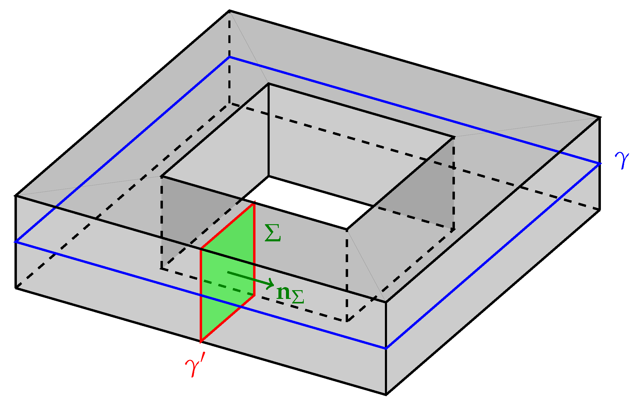
The domain depicted in Figure 2 serves as an example to point out the defect of the trial (41). We assume that there is a toroidal current density $\mathit{J}$, that is $\mathit{J}$ circulates around the hole in the domain. The total current I for a cross section Σ with normal ${\mathit{n}}_{\mathsf{\Sigma }}$ and closed boundary $\partial \mathsf{\Sigma }$ (for instance, the red circle in Figure 2) becomes

$$\begin{array}{cc}\hfill I& ={\int }_{\mathsf{\Sigma }}\mathit{J}·{\mathit{n}}_{\mathsf{\Sigma }}\mathrm{d}\mathsf{\Sigma }={\int }_{\mathsf{\Sigma }}\mathbf{curl}\mathit{H}·{\mathit{n}}_{\mathsf{\Sigma }}\mathrm{d}\mathsf{\Sigma }={\oint }_{\partial \mathsf{\Sigma }}\mathit{H}·\tau \mathrm{d}s\hfill \\ \hfill & ={\oint }_{{\gamma }^{\prime }}\left((\mathit{H}·\mathit{n})\mathit{n}+\mathit{n}\times \mathit{\lambda }\right)·\tau \mathrm{d}s={\oint }_{{\gamma }^{\prime }}\left(\mathit{n}\times {\mathbf{grad}}_{\mathsf{\Gamma }}\psi \times \mathit{n}\right)·\tau \mathrm{d}s\hfill \\ \hfill & ={\oint }_{{\gamma }^{\prime }}\mathbf{grad}\psi ·\tau \mathrm{d}s=0,\hfill \end{array}$$

(42)

where $\mathit{n}$ refers to the domain’s surface Γ and τ is tangent to ${\gamma }^{\prime }$, hence also tangent to Γ. In this derivation, we have used Ampère’s law (1), Stoke’s theorem, the decomposition into normal and tangential surface components of $\mathit{H}$, the representation of λ by means of ${\mathbf{curl}}_{\mathsf{\Gamma }}\psi$, and the fact that ${\gamma }^{\prime }=\partial \mathsf{\Sigma }$ is a closed circle. Clearly, for the given situation, there is a contradiction in that I cannot be zero for the considered non-zero current density. We thus need to augment the trial (41) by adding extra functions.

For domains that are not simply connected, we have to incorporate vector functions along the topological generators. For the case depicted in Figure 2, there are two independent generators (blue and red) and a vector function along the blue one repairs the trial and yields a non-zero total current. For simplicity, it does not hurt to incorporate vector functions along both generators and we know from basic topology that each hole implies two such generators. Let $\mathsf{\Omega }$ have L topological holes and therefore have $2L$ independent generators ${\gamma }_{\ell }$. Along each generator, we define a vector-valued function ${\mathit{\eta }}_{\ell }$ such that

$${\oint }_{{\gamma }_k^{\prime }}{\mathit{\eta }}_{\ell }·\mathit{\tau }\mathrm{d}s={\delta }_{k\ell },$$

(43)

where ${\gamma }_k^{\prime }$ is the dual path to ${\gamma }_k$ in the same way as in Figure 2. Note that ${({\gamma }_k^{\prime })}^{\prime }={\gamma }_k$. Finally, we state the augmented trial for the surface magnetic field

$$\mathit{\lambda }(x)\approx {\mathbf{curl}}_{\mathsf{\Gamma }}{\psi }_h(x)+\sum _{\ell =1}^{2L}{\alpha }_{\ell }{\mathit{\eta }}_{\ell }.$$

(44)

We must discuss how to obtain these global functions ${\mathit{\eta }}_{\ell }$. Here, we work with the algorithms developed in [11], which only require a surface mesh if all $2L$ generators are included.

3.2. Spatial Discretisation

By splitting spatial and temporal discretisation, we summarise the spatial approximations

$$\begin{array}{cc}\hfill \mathit{A}(x,t)& \approx \sum a_i(t){\mathit{w}}_i(x)\hfill \\ \hfill \mathit{\lambda }(x,t)& \approx \sum {\psi }_j(t){\mathbf{curl}}_{\mathsf{\Gamma }}{\phi }_j(x)+\sum {\alpha }_{\ell }(t){\mathit{\eta }}_{\ell }.\hfill \end{array}$$

(45)

Introducing these FE approximations into the system (38) yields the system of equations

$$\left[\begin{array}{cc}\underset{¯}{M}& \underset{¯}{0}\\ \underset{¯}{0}& \underset{¯}{0}\end{array}\right]{\partial }_t\left[\begin{array}{c}\underset{¯}{a}(t)\\ \underset{¯}{\psi }(t)\end{array}\right]+\left[\begin{array}{c}\underset{¯}{h}(\underset{¯}{a})\\ \underset{¯}{0}\end{array}\right]+\left[\begin{array}{cc}\underset{¯}{W}& {\underset{¯}{K}}^{\top }\\ \underset{¯}{K}& -\underset{¯}{V}\end{array}\right]\left[\begin{array}{c}\underset{¯}{a}(t)\\ \underset{¯}{\psi }(t)\end{array}\right]=\left[\begin{array}{c}\underset{¯}{f}(t)\\ \underset{¯}{0}\end{array}\right].$$

(46)

This system still depends continuously on time and is non-linear in the term $\underset{¯}{h}(\underset{¯}{a})$ due to the possible non-linear relation between $\mathit{B}$- and $\mathit{H}$-fields.

Remark 3.

Equation (46) does not explicitly reveal the occurrence of the weights ${\alpha }_{\ell }$ associated to the additional vector-fields ${\mathit{\eta }}_{\ell }$. These extra degrees of freedom are either subsumed in the coefficients $\underset{¯}{\psi }$ or they have been removed from the system of equations by simple elimination. In the latter case, a matrix of dimension $2L\times 2L$ is inverted prior to the solution process and the matrices representing the boundary integral operators are modified accordingly.

3.3. Time Integration

For simplicity we use here the Euler backward time integration method

$${\partial }_{t}y=f(y,t)\to y_{n+1}=y_n+\mathsf{\Delta }tf(y_{n+1},t_{n+1}),$$

(47)

where $y_n$ approximates $y(t_n)$ and $t_n=n\mathsf{\Delta }t$ is the n-th time point along an equidistant time grid with step size $\mathsf{\Delta }t$.

Remark 4.

The presented method is not restricted to the Euler backward integration nor to equidistant time grids. The preceding choices are only made in order to keep the presentation of the algorithms as simple as possible.

Based on this approach, system (46) becomes

$$\frac{1}{\mathsf{\Delta }t}\left[\begin{array}{cc}\underset{¯}{M}& \underset{¯}{0}\\ \underset{¯}{0}& \underset{¯}{0}\end{array}\right]\left[\begin{array}{c}{\underset{¯}{a}}_{n+1}\\ {\underset{¯}{\psi }}_{n+1}\end{array}\right]+\left[\begin{array}{c}\underset{¯}{h}({\underset{¯}{a}}_{n+1})\\ \underset{¯}{0}\end{array}\right]+\left[\begin{array}{cc}\underset{¯}{W}& {\underset{¯}{K}}^{\top }\\ \underset{¯}{K}& -\underset{¯}{V}\end{array}\right]\left[\begin{array}{c}{\underset{¯}{a}}_{n+1}\\ {\underset{¯}{\psi }}_{n+1}\end{array}\right]=\left[\begin{array}{c}{\underset{¯}{f}}_{n+1}\\ \underset{¯}{0}\end{array}\right]+\frac{1}{\mathsf{\Delta }t}\left[\begin{array}{cc}\underset{¯}{M}& \underset{¯}{0}\\ \underset{¯}{0}& \underset{¯}{0}\end{array}\right]\left[\begin{array}{c}{\underset{¯}{a}}_n\\ {\underset{¯}{\psi }}_n\end{array}\right]$$

(48)

with suitable initial conditions for ${\underset{¯}{a}}_0=\underset{¯}{a}(0)$.

3.4. Newton Method

System (48) is possibly non-linear as represented by the term $\underset{¯}{h}({\underset{¯}{a}}_{n+1})$. Therefore, within each time step it is necessary to iteratively determine the new solution vector by means of a non-linear equation solver. We chose a Newton method with optional line search in order to solve (48). To this end, we write

$$\underset{¯}{g}(\underset{¯}{x})=\underset{¯}{L}\underset{¯}{x}+\underset{¯}{n}(\underset{¯}{x})+\underset{¯}{f}=0$$

(49)

in terms of ${\underset{¯}{x}}^{\top }=\left[{\underset{¯}{a}}_{n+1}^{\top }{\underset{¯}{\psi }}_{n+1}^{\top }\right]$. The meaning of the symbols $\underset{¯}{L}$, $\underset{¯}{n}$, and $\underset{¯}{f}$ should be clear when comparing to Equation (48), where the non-linearity is contained in $\underset{¯}{n}(\underset{¯}{x})$. The Newton method now reads

$${\underset{¯}{x}}^{(k+1)}={\underset{¯}{x}}^{(k)}+{\beta }^{(k)}\mathsf{\Delta }\underset{¯}{x}\mathrm{with}\left[\underset{¯}{L}+\underset{¯}{J}({\underset{¯}{x}}^{(k)})\right]\mathsf{\Delta }\underset{¯}{x}=\underset{¯}{f}-\underset{¯}{L}{\underset{¯}{x}}^{(k)}-\underset{¯}{n}({\underset{¯}{x}}^{(k)}).$$

(50)

In this algorithm, ${\underset{¯}{x}}^{(k)}$ denotes the current iterate, $\underset{¯}{J}$ the Jacobian related to $\underset{¯}{n}(\underset{¯}{x})$, and ${\beta }^{(k)}\in (0,1]$ is a weighting parameter, which is obtained by means of a one-dimensional minimisation of a scalar-valued cost function $\mathsf{\Phi }(\beta )=\widehat{\mathsf{\Phi }}({\underset{¯}{x}}^{(k)}+\beta \mathsf{\Delta }\underset{¯}{x})$. Ideally, ${\mathrm{D}}_{\underset{¯}{x}}\widehat{\mathsf{\Phi }}=\underset{¯}{g}(\underset{¯}{x})$ and we choose

$$\widehat{\mathsf{\Phi }}(\underset{¯}{x})=\frac{1}{2}{\underset{¯}{x}}^{\top }\underset{¯}{L}\underset{¯}{x}+e(\underset{¯}{x})+{\underset{¯}{x}}^{\top }\underset{¯}{f},$$

(51)

where $e(x)$ denotes the magnetostatic energy contained in $\mathsf{\Omega }$. In particular, we use the line search algorithm presented in [12] in order to determine the weighting parameter ${\beta }^{(k)}$ in the k-th Newton iteration of the form (50).

4. Solution of Linear System of Equations

Plugging everything together, the final system of equations in each Newton step of each time integration step has the form

$$\begin{array}{c}\left[\begin{array}{cc}\frac{1}{\mathsf{\Delta }t}\underset{¯}{M}+{\underset{¯}{J}}_{n+1}^{(k)}+\underset{¯}{W}& {\underset{¯}{K}}^{\top }\\ \underset{¯}{K}& -\underset{¯}{V}\end{array}\right]\left[\begin{array}{c}\mathsf{\Delta }\underset{¯}{a}\\ \mathsf{\Delta }\underset{¯}{\psi }\end{array}\right]=\hfill \\ \left[\begin{array}{c}{\underset{¯}{f}}_{n+1}\\ \underset{¯}{0}\end{array}\right]-\frac{1}{\mathsf{\Delta }t}\left[\begin{array}{cc}\underset{¯}{M}& \underset{¯}{0}\\ \underset{¯}{0}& \underset{¯}{0}\end{array}\right]\left[\begin{array}{c}{\underset{¯}{a}}_{n+1}^{(k)}-{\underset{¯}{a}}_n\\ {\underset{¯}{\psi }}_{n+1}^{(k)}-{\underset{¯}{\psi }}_n\end{array}\right]-\left[\begin{array}{c}\underset{¯}{h}({\underset{¯}{a}}_{n+1}^{(k)})\\ \underset{¯}{0}\end{array}\right]-\left[\begin{array}{cc}\underset{¯}{W}& {\underset{¯}{K}}^{\top }\\ \underset{¯}{K}& -\underset{¯}{V}\end{array}\right]\left[\begin{array}{c}{\underset{¯}{a}}_{n+1}^{(k)}\\ {\underset{¯}{\psi }}_{n+1}^{(k)}\end{array}\right].\hfill \end{array}$$

(52)

The system matrix in (52) is symmetric and indefinite. Furthermore, there are two major difficulties when it comes to solving this system:

• The matrix ${\underset{¯}{J}}_{n+1}^{(k)}$, that is, the linearisation of $\underset{¯}{h}(\underset{¯}{a})$ at ${\underset{¯}{a}}_{n+1}^{(k)}$, has a large kernel due to the fact that $\mathbf{curl}\mathbf{grad}=\mathit{0}$. In case there are non-conducting regions, or in other words $supp(\sigma )⊊\mathsf{\Omega }$, this deficiency carries over to the entire top-left block of the system matrix. In case of a direct solver, one would need to classify the degrees of freedom on the finite element mesh and eliminate the redundant ones, see [13]. For iterative solvers, on the other hand, careful preconditioning is needed as discussed below.
• The matrices $\underset{¯}{W}$, $\underset{¯}{K}$, and $\underset{¯}{V}$ are fully populated. This implies a quadratic complexity for storage and cost of matrix-vector products. Since a direct solution is complicated from the onset—see the previous point—it can be ruled out completely when considering its cubic complexity due to the boundary element matrices. In case of an iterative solution, only the actions of these matrices on a given vector need to be calculated.

4.1. Fast Multipole Method

The second of the above-listed difficulties, the fully populated BEM matrices, is addressed here by using a fast multipole method [14]. Without going too much into the details, we will give an outline of the mechanisms of the method. To begin with, each surface degree of freedom is associated with a geometric location and these locations are hierarchically clustered, typically by using octrees. This means that the point cloud representing the degrees of freedom is partitioned into eight similar cubes and each cube, in turn, is subdivided in the same way if it is not empty and contains more than a predefined number of points. The left image in Figure 3 indicates this partitioning by the different colours given to each point the belongs to a cluster, that is one of these boxes, of the same partitioning level. Each cluster has direct neighbours that define its near-field and the remaining clusters of the same level thus belong to its far field. The key idea is now that the interaction between a cluster and its far field can be approximated. Moreover, the near-field clusters become far field after a further partition which gives rise to a multi-level scheme, as indicated by the right image in Figure 3. By means of spherical harmonics, one can make use of an expansion with the structure

$$\frac{1}{|x-y|}=\sum _{i=0}^{\infty }{f}_i(x)g_i(y)$$

(53)

and obtain an approximation by truncation of the infinite series. Expression (53) is far more complex in reality and only used here to transmit the basic idea of fast multipole approximations. The level of truncation of this sum together with the corresponding geometric constellation allows for a precise error estimate [14] such that the approximation error of the fast multipole can be well controlled. Overall, the fast multipole method exhibits a linear complexity in terms of the surface degrees of freedom.

4.2. Preconditioning

As pointed out earlier, iterative solution methods are the right choice in order to solve system (52); however, to keep the numerical costs bounded it is essential to use preconditioners, which ideally control the conditioning of the system independent of mesh refinement. Methods that come close to this ideal are algebraic multigrid methods [15] and operator preconditioning [16]. In particular, we choose a preconditioner $\underset{¯}{P}$ of the form

$$\underset{¯}{P}=\left[\begin{array}{c}{\underset{¯}{P}}_A\\ & {\underset{¯}{P}}_V\end{array}\right].$$

(54)

Here, ${\underset{¯}{P}}_A$ is based on [17] and hence a modification of an algebraic multigrid scheme. The BEM matrix $\underset{¯}{V}$ on the other hand has the same coefficients as the discretisation of the hypersingular operator for Laplace equation and we therefore make use of the operator preconditioning as advocated in [16] in order to realise ${\underset{¯}{P}}_V$. Since the preconditioner ${\underset{¯}{P}}_V$ is itself a boundary element matrix, we also make use of the fast multipole method for its application with linear numerical cost.

5. Force Computation

With the aim of analysing the mechanical behaviour of electromagnetic devices, it is of utmost importance to calculate magnetic forces. Classically, the key player in the interaction is the Lorentz force density ${\mathit{f}}_L=\mathit{J}\times \mathit{B}$, where here and in the following, the electric part of this force is being neglected. Obviously, this force is zero in the absence of currents and can therefore not account for, e.g., the forces between two permanent magnets; therefore, we make use of the approach given in [18] and consider a force as a specific derivative of the magnetic energy with respect to an (imaginary) velocity field. The gist is given by the force component in direction of $\mathit{v}$,

$$\mathit{F}·\mathit{v}=-{\int }_{\mathsf{\Omega }}\sigma (\mathit{B},\mathit{H}):\mathbf{grad}{\mathit{v}}^{\top }\mathsf{d}\mathsf{\Omega }.$$

(55)

In this equation, $\mathit{v}$ denotes the velocity that is power-adjoint to the force of interest and $\sigma$ is the Maxwell stress tensor

$$\sigma =\mathit{B}\otimes \mathit{H}-\left(\mathit{H}·\mathit{B}-w(\mathit{B})\right)\mathit{I}$$

(56)

with the magnetostatic energy density $w(\mathit{B})$ (11). Note that the term in brackets is often referred to as co-energy. This tensor is symmetric due to the assumption of an isotropic material and, hence, the co-linearity of $\mathit{B}$ and $\mathit{H}$. By integration of parts, we obtain

$$\begin{array}{c}\hfill \mathit{F}·\mathit{v}=-{\int }_{\mathsf{\Omega }}div\left[\sigma \mathit{v}\right]-div\sigma ·\mathit{v}\mathsf{d}\mathsf{\Omega }=-{\int }_{\mathsf{\Gamma }}\left[\sigma \mathit{v}\right]·\mathit{n}\mathsf{d}\mathsf{\Gamma }+{\int }_{\mathsf{\Omega }}div\sigma ·\mathit{v}\mathsf{d}\mathsf{\Omega }\end{array}$$

(57)

and for the domain part the integrand becomes

$$\begin{array}{cc}\hfill div\sigma & =div\left[\mathit{B}\otimes \mathit{H}-\left(\mathit{H}·\mathit{B}-w(\mathit{B})\right)\mathit{I}\right]\hfill \\ \hfill & =(div\mathit{B})\mathit{H}+(\mathbf{grad}\mathit{H})\mathit{B}-(\mathbf{grad}{\mathit{H}}^{\top })\mathit{B}-{(\mathbf{grad}\mathit{B})}^{\top }\mathit{H}+\mathbf{grad}w\hfill \\ \hfill & =0\mathit{H}+(\mathbf{curl}\mathit{H})\times \mathit{B}+\left(\mathbf{grad}w-\mathbf{grad}{B}^{\top }\mathit{H}\right)\hfill \\ \hfill & =\mathit{J}\times \mathit{B},\hfill \end{array}$$

(58)

which is the Lorentz force density ${\mathit{f}}_L$. Clearly, if there are no currents (magnetostatics) the only non-zero contribution to the force has to come from the boundary term when using the last part of (57). In order to compute the ℓ-th component of a nodal force ${\mathit{F}}^k[\ell ]$ at the node $x^k$ of the finite element mesh, we set $\mathit{v}={\phi }_k{\mathit{e}}_{\ell }$ with the nodal hat function associated to $x^k$ and the ℓ-th Cartesian unit vector. Therefore, we have the following options to calculate the k-th nodal force

$$\begin{array}{cc}\hfill {\mathit{F}}^k& =-{\int }_{supp{\phi }_k}\sigma (\mathit{B},\mathit{H})\mathbf{grad}{\phi }^k\mathrm{d}\mathsf{\Omega }\hfill \end{array}$$

(59)

$$\begin{array}{cc}\hfill & ={\int }_{supp{\phi }_k\cap \mathsf{\Omega }}{\mathit{f}}_L{\phi }^k\mathrm{d}\mathsf{\Omega }-{\int }_{supp{\phi }_k\cap \mathsf{\Gamma }}{\sigma }^{\top }\mathit{n}{\phi }^k\mathrm{d}\mathsf{\Gamma }.\hfill \end{array}$$

(60)

The first variant, (59), is commonly referred to as the principle of virtual work in the finite element community and gives good accuracy. One has to bear in mind that for the underlying principles [18] to be valid, the velocity field $\mathit{v}$ has to be continuous. This implies that a nodal force at the boundary of a domain can only be calculated by (60). To be more precise, the expression (60) contains the Lorentz force density ${\mathit{f}}_L$ and the boundary part stemming from contributions from ${\mathsf{\Omega }}^{+}$, that is from outside of $\mathsf{\Omega }$ where $\mathit{B}={\mu }_0\mathit{H}$. Therefore, we can rewrite the integrand of the boundary term as

$$\begin{array}{cc}\hfill {\mathit{\sigma }}^{\top }\mathit{n}& =\left(\mathit{H}\otimes \mathit{B}\right)\mathit{n}-\left[\mathit{H}·\mathit{B}-\frac{1}{2}\mathit{H}·\mathit{B}\right]\mathit{n}\hfill \\ \hfill & =\left(\mathit{B}·\mathit{n}\right)\mathit{H}-\frac{1}{2}\left(\mathit{B}·\mathit{H}\right)\mathit{n}\hfill \\ \hfill & =B_n\left(H_n\mathit{n}+\mathit{n}\times \mathit{\lambda }\right)-\frac{1}{2}\left(B_n{H}_n+(\mathit{n}\times {\mathit{B}}_{\times })·(\mathit{n}\times \mathit{\lambda })\right)\mathit{n}\hfill \\ \hfill & =B_n\left(\frac{1}{{\mu }_0}{B}_n\mathit{n}+\mathit{n}\times \mathit{\lambda }\right)-\frac{1}{2}\left(\frac{1}{{\mu }_0}{B}_n{B}_n+(\mathit{n}\times {\mu }_0\mathit{\lambda })·(\mathit{n}\times \mathit{\lambda })\right)\mathit{n}\hfill \\ \hfill & =\frac{1}{2}\left[\frac{1}{{\mu }_0}{B}_n^2-{\mu }_0\mathit{\lambda }·\mathit{\lambda }\right]\mathit{n}+B_n\mathit{n}\times \mathit{\lambda }.\hfill \end{array}$$

(61)

Hence, we can use tangential magnetic field $\mathit{\lambda }$ from the exterior (BEM) part of the simulation and the normal magnetic flux intensity $B_n$ from the interior (FEM) part.

6. Results

In this section, we present a few numerical simulations that demonstrate the accuracy of the proposed method and, in addition, emphasise its versatility in combination with moving parts. The convergence of the method has been demonstrated elsewhere [19]. All examples have been carried out with lowest-order space discretisation and a Euler-backward time integration. Not mentioned in the derivations of this work is that current excitations from spatially separate coil domains can also be incorporated by means of the Biot–Savart law [20]. In this case, excitation fields ${\mathit{A}}_s$ and ${\mathit{B}}_s=\mathbf{curl}{\mathit{A}}_s$ are pre-computed for the given coil and current distribution, which can then be incorporated by means of the transmission conditions (9). The advantage is that the coil domains need not be incorporated directly into the computation and thus the system size is reduced.

We emphasise that in every of the presented examples only the visualised solid parts require a volume mesh. The proposed method effectively eliminates the discretisation of free space and we make full use of this advantage.

6.1. Force between Permanent Magnets

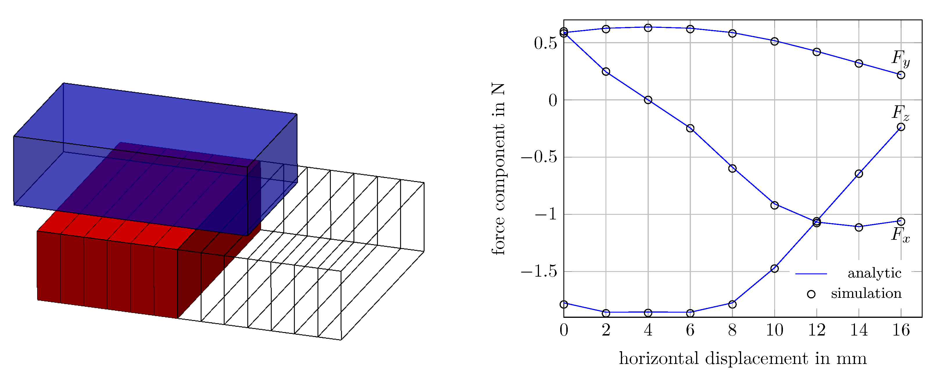
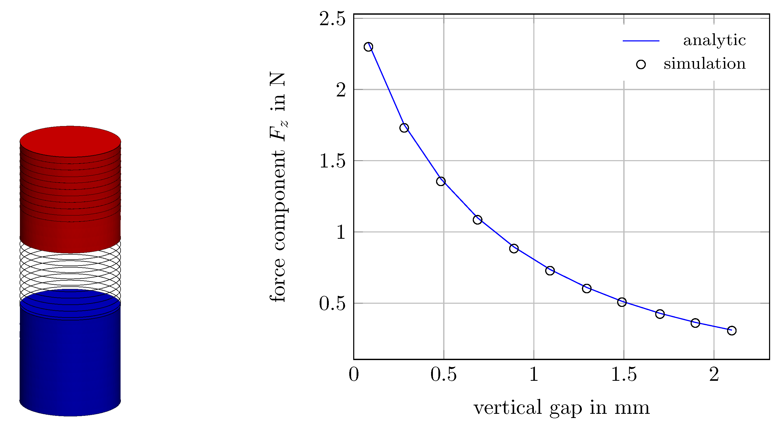
To begin with, we look at the force between two permanent magnets. In particular, the case of two rectangular parallelepipeds with parallel axes and the case of two cylindrical magnets with the same central axis are analysed. As reference for these cases, the analytic solutions given in [21] for the parallelepipeds and in [22] for the cylindrical magnets are used. The left images in Figure 4 and Figure 5 show the simulation setup where in both cases the magnetisation is the vertical (z) direction. The right plots in these Figures show the outcome of the analytical model of the references and the simulated results for various positions of the red magnets. Plotted are the total force acting on the blue magnets. The precise setups of the models, that is magnetisation value and geometry parameters, are given in the references [21,22] where, in addition, experimental validations of these models have been carried out.

In both cases, we can observe an excellent agreement between analytic model and simulation results. Note that here there is no Lorentz force and we have used expression (60) with (61) for the calculation of the nodal forces whose sum provides the presented results.

6.2. TEAM 24

Here, we consider the TEAM 24 benchmark problem as defined in [23]. The problem domain consists of a stator and rotor part and two coils surrounding the poles of the stator. The rotor is fixed at an angle of 23 ${}^{\circ }$ rotated from alignment of the poles. The geometry is depicted in the left image in Figure 6. Here, the current-driven version is carried out using the current-time relation given in [23]. The currents asymptotically converges to a steady value such that time-dependent effects disappear. The material behaviour in the rotor and stator regions is characterised by the B-H curve given in the right image in Figure 6. Note that it has also been confirmed in other studies that the provided data points of [23] do not describe the material sufficiently; the region between zero and the first data point are especially problematic: drawing a straight line from zero to this first point or a somewhat curved approximation curve lead to significant differences in the outcome. To alleviate this issue, we make use of the so-called Fröhlich model, see [24], that gives a global approximation of the $B(H)$ relation and is also plotted in Figure 6.

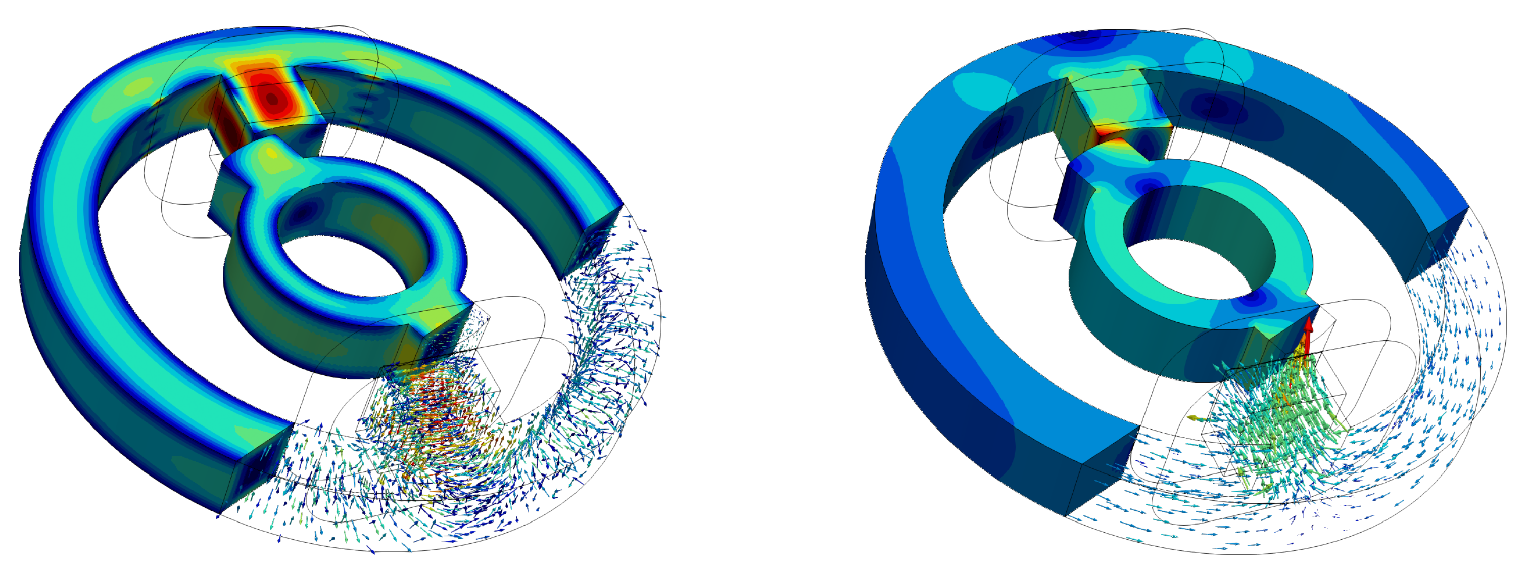
Figure 7 shows some images of the results of the simulation. We display the induced currents ${\mathit{J}}_e$ at $t=0.03\mathrm{s}$ in the left image and the B-field at $t=0.3\mathrm{s}$ in the right image. Note, that the induced currents disappear for large times since the system approaches a steady state. Moreover, the magnitude of the B-field is with almost $2.5\mathrm{T}$ well in the saturation phase when considering the $B(H)$ curve in Figure 6.

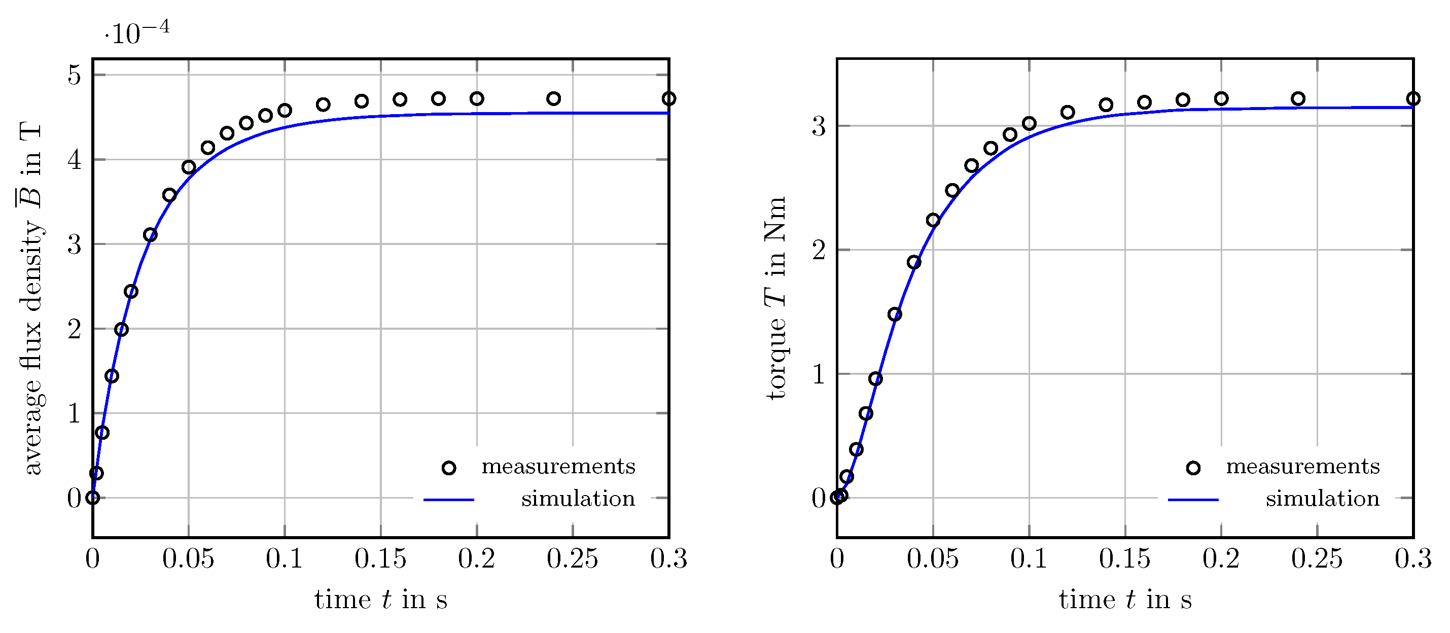
The proposition of this benchmark [23] also contains measured experimental data for the validation of the simulation results. To this end, we consider the average magnetic flux density, $\overline{B}={\int }_S\mathit{B}·{\mathit{n}}_{S}S/\left|S\right|$, through a specified surface S that is basically the cross section of a rotor pole. The comparison of measured and simulated results is given in the left plot in Figure 8. In addition, the integral torque T on the rotor domain has been measured and calculated for the right plot of the same figure. We can observe a very good agreement between experimental and simulated data with deviations of less than $4\%$ for large times in both considered quantities.

6.3. Eddy-Current Brake

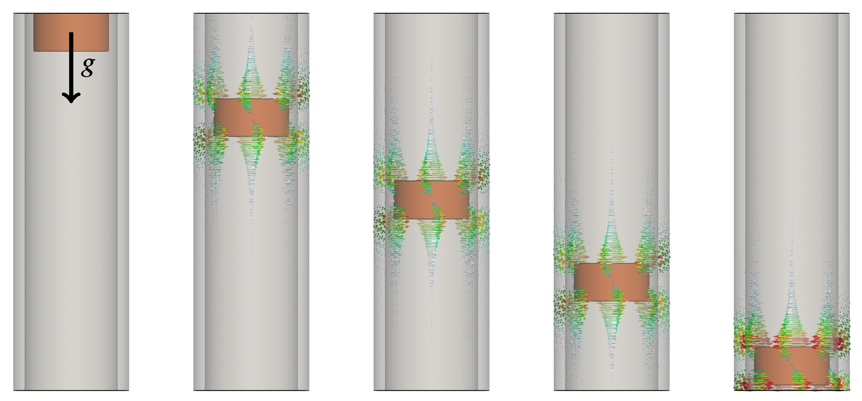
Next, we consider the simplest model of an eddy-current brake: a permanent magnet falling through a copper pipe. This resembles a classic experiment from high school physics and demonstrates induction mechanisms. The basic principle is depicted in the left image in Figure 9. A permanent magnet that falls due to gravity incurs a temporarily changing magnetic field, and by virtue of Faraday’s law (2), creates an electric field. This induces currents in the copper pipe due to Ohm’s law (5). These currents, in turn, create a magnetic field due to Ampère’s law (1), which brakes the magnet.

Snapshots of the falling magnet are displayed in Figure 10, which show the induced currents in the copper pipe near the magnet. One can see the circumferential currents with direction above opposed to below the magnet position, in accordance with the left image in Figure 9. The snapshots are given at equidistant time points and thus demonstrate the constant velocity of the magnet as opposed to a constant acceleration in free fall. This is substantiated by means of the plot in Figure 9. While inside the tube, the magnet falls with a constant velocity whose magnitude agrees very well with the simplified analytic model developed in [25].

6.4. Electromagnetic Launcher

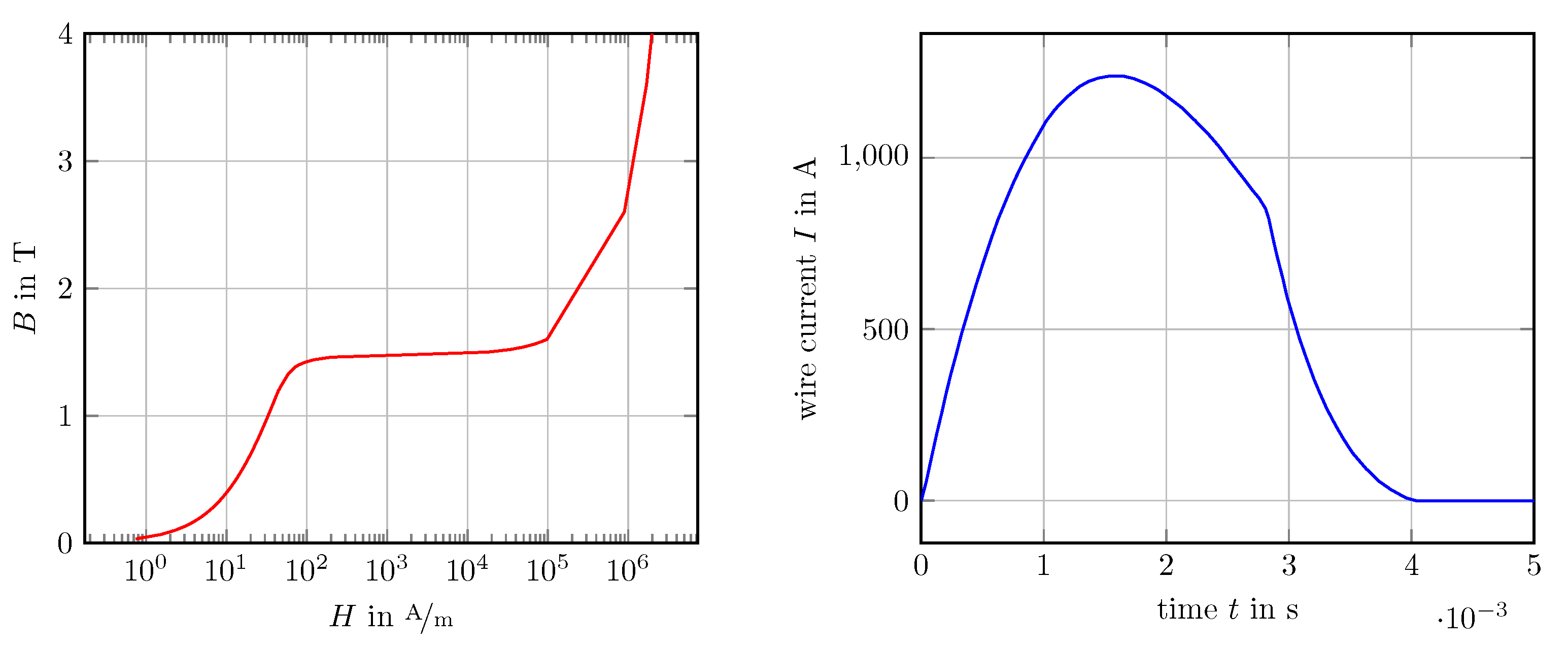
In this example, we consider an application in which electromagnetic forces are used to accelerate a conducting, magnetic object. In its most simple version, a coil is temporarily subject to a direct current that generates a strong magnetic field. This, in turn, magnetises the projectile, which is then being sucked into the coil. If the current is turned off at the right time, this acceleration is never reversed and the object keeps moving in the desired direction. Coil guns typically work with this principle and often contain a series of such coils that further accelerate the object by precise timing of activation and deactivation of the currents. In the presented example, we use the setup of [26] with a coil of 203 turns and a current density as given in the left plot of Figure 11. The material behaviour of the projectile is described the $B(H)$-relation as in the right plot of the same figure.

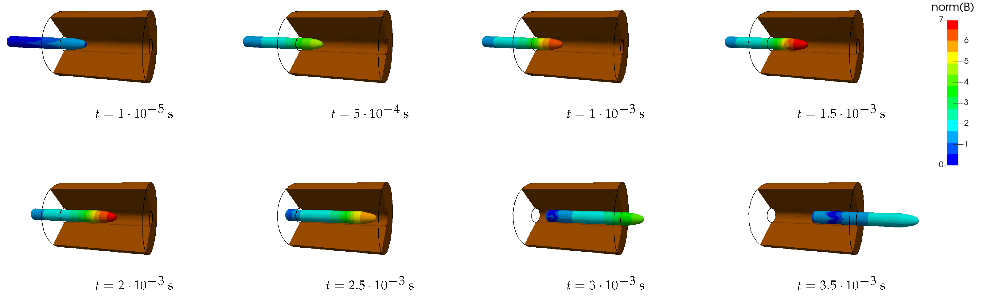
Figure 12 shows eight snapshots of the simulation, after the first time step of size $\mathsf{\Delta }t=1\times {10}^{-5}$ s, then at $t_i=50i\mathsf{\Delta }t$ with $i=1,\dots ,7$. Clearly, the projectile hardly moves for the first four considered time points and then moves noticeably to the right.

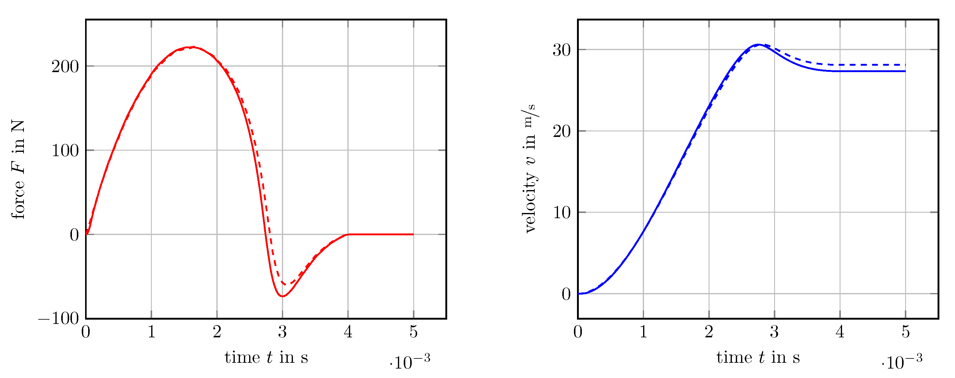
The particular details of the projectile’s motion is given in Figure 13 with the integral force on the object and its velocity over the considered time. For comparison, the simulation has been performed as a magnetostatic axisymmetric problem with the software package FEMM [27]. It is based on the FEM, and therefore the air region has to be re-meshed in each time step.

Remark 5.

The presented simulation here differs from the work presented in [26] in several aspects. In the reference, the term $\sigma {\partial }_t\mathit{A}$ of Equation (8) is replaced by $\sigma ({\partial }_t\mathit{A}-\mathit{v}\times \mathbf{curl}\mathit{A})$, which stems from the coordinate change due to the motion of the projectile where $\mathit{v}$ is the velocity vector of the projectile. Moreover, drag forces of structure $\frac{1}{2}CS{\rho }_{air}\mathit{v}·\mathit{v}$ with a shape factor C and the cross section S have been included. We have incorporated both these effects but the difference to the outcome without them is negligible, in fact less than 0.1% difference has been obtained in the terminal velocity. At last, in [26] a voltage-driven analysis was carried out in which a circuit equation is coupled (via its inductivity) with an eddy-current system. Instead, we have simply taken the measured current distribution of that reference in order to drive the coil.

6.5. Magnetic Metal Forming

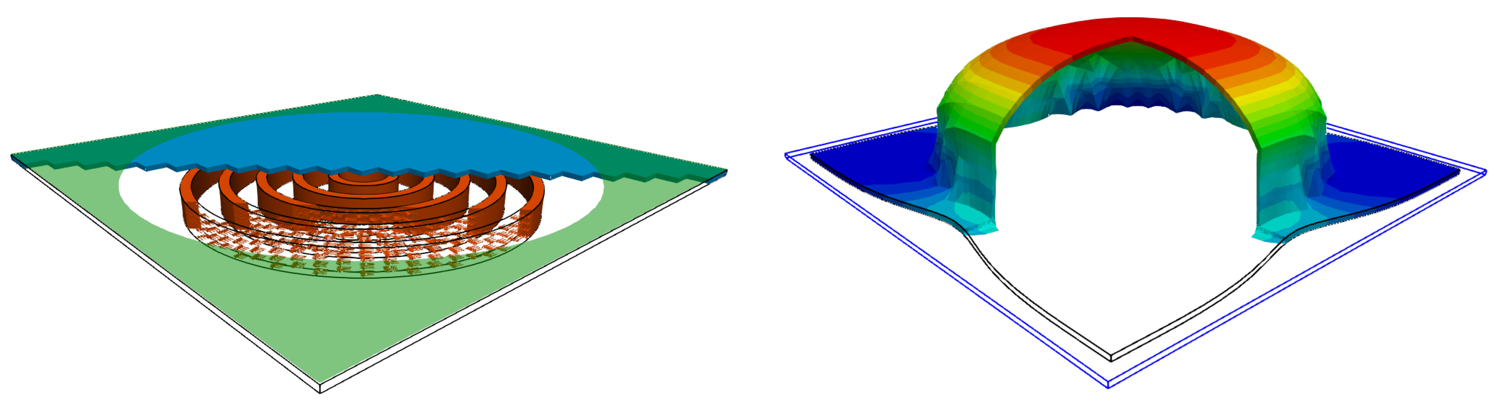
Another application of magnetic forces is the so-called magnetic metal forming in which a sudden release of large current into a well-designed system of coils very quickly generates large opposing forces in a nearby placed work piece. This mechanism can be used to form metal and many variants of it are presented in [28]. We will not immerse ourselves into the depths and technicalities of this process, but just present a simple simulation that demonstrates the mechanism. Therefore, the setup displayed in the left image of Figure 14 is used: the work piece (blue) is placed above multiple coils (red) and subject to a vertical displacement constraint (green). In order to analyse the work piece, we make use of continuum plasticity with finite strains [29]. The application of the large currents induce the deforming magnetic forces that push the work piece away from the coils. The final state of deformation is shown in the right image in Figure 14. Clearly, the conducting plate has been pushed through the hole of the displacement constraints and assumed a new shape.

7. Conclusions

A symmetric coupling formulation between the finite element and the boundary element method for eddy-current problems has been presented. The solid parts of the electrical devices are tackled by the FEM, which can easily account for material non-linearities. The surrounding domain is represented by the BEM via a surface-only discretisation. As the main feature of this approach, no air-mesh or even re-meshing is required if components are moving or are subject to large deformations. We use Nédélec functions for the spatial discretisation and incorporate additional vector spaces in the case of multiply connected domains. The usually non-linear behaviour of the component’s material is tackled by a Newton method involving a line search algorithm. By using the fast multipole method and iterative solution methods in connection with suitable preconditioners, the presented method has an optimal complexity. This means that the memory and time required depend linearly on the number of degrees of freedom.

To analyse the mechanical behaviour of the solid parts, the calculation of magnetic forces is of great importance and accurately achieved by using the flux intensity from the interior and the tangential magnetic field from the exterior domain. The implemented method has been validated by a set of benchmarks and was used to calculate some practical examples.

In summary, the features of the proposed coupling scheme make it an ideal approach for the investigation of the mechanical behaviour of electrical devices. In order to set up the simulation, the design engineer can operate on the CAD model and does not have to bother with the surrounding domain and its descretisation.

References

- Sauter, S.A.; Schwab, C. Boundary Element Methods; Springer: Berlin/Heidelberg, Germany, 2010. [Google Scholar]
- Zienkiewicz, O.; Kelly, D.; Bettess, P. The coupling of the finite element method and boundary solution procedures. Int. J. Numer. Methods Eng. 1977, 11, 355–375. [Google Scholar] [CrossRef]
- Johnson, C.; Nédélec, J. On the coupling of boundary integral and finite element methods. Math. Comput. 1980, 35, 1063–1079. [Google Scholar] [CrossRef]
- Bossavit, A.; Verite, J.C. A mixed FEM-BIEM method to solve 3-D eddy-current problems. IEEE Trans. Magn. 1982, 18, 431–435. [Google Scholar] [CrossRef]
- Kuhn, M.; Steinbach, O. Symmetric coupling of finite and boundary elements for exterior magnetic field problems. Math. Methods Appl. Sci. 2002, 25, 357–371. [Google Scholar] [CrossRef]
- Hiptmair, R. Symmetric coupling for eddy current problems. SIAM J. Numer. Anal. 2002, 40, 41–65. [Google Scholar] [CrossRef] [Green Version]
- Hiptmair, R.; Sterz, O. Current and voltage excitations for the eddy current model. Int. J. Numer. Model. Electron. Netw. Devices Fields 2005, 18, 1–21. [Google Scholar] [CrossRef] [Green Version]
- Monk, P. Finite Element Methods for Maxwell’s Equations; Oxford University Press: Oxford, UK, 2003. [Google Scholar]
- Chen, Q.; Konrad, A. A review of finite element open boundary techniques for static and quasi-static electromagnetic field problems. IEEE Trans. Magn. 1997, 33, 663–676. [Google Scholar] [CrossRef]
- Ern, A.; Guermond, J.L. Theory and Practice of Finite Elements; Springer Science & Business Media: Berlin/Heidelberg, Germany, 2013; Volume 159. [Google Scholar]
- Hiptmair, R.; Ostrowski, J. Generators of H1(Γh,) for Triangulated Surfaces: Construction and Classification. SIAM J. Comput. 2002, 31, 1405–1423. [Google Scholar] [CrossRef]
- Moré, J.J.; Thuente, D.J. Line search algorithms with guaranteed sufficient decrease. ACM Trans. Math. Softw. TOMS 1994, 20, 286–307. [Google Scholar] [CrossRef]
- Manges, J.B.; Cendes, Z.J. A generalized tree-cotree gauge for magnetic field computation. IEEE Trans. Magn. 1995, 31, 1342–1347. [Google Scholar] [CrossRef]
- Greengard, L.; Rokhlin, V. A new version of the fast multipole method for the Laplace equation in three dimensions. Acta Numer. 1997, 6, 229–269. [Google Scholar] [CrossRef]
- Ruge, J.W.; Stüben, K. Algebraic multigrid. In Multigrid Methods; SIAM: Philadelphia, PA, USA, 1987; pp. 73–130. [Google Scholar]
- Steinbach, O.; Wendland, W.L. The construction of some efficient preconditioners in the boundary element method. Adv. Comput. Math. 1998, 9, 191–216. [Google Scholar] [CrossRef]
- Hiptmair, R.; Xu, J. Nodal auxiliary space preconditioning in H(curl) and H(div) spaces. SIAM J. Numer. Anal. 2007, 45, 2483–2509. [Google Scholar] [CrossRef]
- Henrotte, F.; Hameyer, K. A theory for electromagnetic force formulas in continuous media. IEEE Trans. Magn. 2007, 43, 1445–1448. [Google Scholar] [CrossRef]
- Kielhorn, L.; Rüberg, T.; Zechner, J. Simulation of electrical machines: A FEM-BEM coupling scheme. COMPEL Int. J. Comput. Math. Electr. Electron. Eng. 2017, 36, 1540–1551. [Google Scholar] [CrossRef] [Green Version]
- Jackson, J.D. Classical Electrodynamics, 3rd ed.; Wiley: New York, NY, USA, 1999. [Google Scholar]
- Akoun, G.; Yonnet, J.P. 3D analytical calculation of the forces exerted between two cuboidal magnets. IEEE Trans. Magn. 1984, 20, 1962–1964. [Google Scholar] [CrossRef]
- Vokoun, D.; Beleggia, M.; Heller, L.; Šittner, P. Magnetostatic interactions and forces between cylindrical permanent magnets. J. Magn. Magn. Mater. 2009, 321, 3758–3763. [Google Scholar] [CrossRef]
- Allen, N.; Rodger, D. Description of TEAM Workshop Problem 24: Nonlinear time-transient rotational test rig. In Proceedings of the TEAM Workshop in the Sixth Round; 1996; pp. 57–60. Available online: http://www.compumag.org/jsite/images/stories/TEAM/problem24.pdf (accessed on 30 May 2021).
- Trutt, F.C.; Erdelyi, E.A.; Hopkins, R.E. Representation of the magnetization characteristic of DC machines for computer use. IEEE Trans. Power Appar. Syst. 1968, 665–669. [Google Scholar] [CrossRef]
- Levin, Y.; da Silveira, F.L.; Rizzato, F.B. Electromagnetic braking: A simple quantitative model. Am. J. Phys. 2006, 74, 815–817. [Google Scholar] [CrossRef] [Green Version]
- Leubner, K.; Laga, R.; Doležel, I. Advanced model of electromagnetic launcher. Power Eng. Electr. Eng. 2015, 13, 223–229. [Google Scholar] [CrossRef]
- Baltzis, K. The FEMM Package: A Simple, Fast, and Accurate Open Source Electromagnetic Tool in Science and Engineering. J. Eng. Sci. Technol. Rev. 2008, 1, 83–89. [Google Scholar] [CrossRef]
- Psyk, V.; Risch, D.; Kinsey, B.L.; Tekkaya, A.E.; Kleiner, M. Electromagnetic forming—A review. J. Mater. Process. Technol. 2011, 211, 787–829. [Google Scholar] [CrossRef]
- Simo, J.C. Numerical analysis and simulation of plasticity. Handb. Numer. Anal. 1998, 6, 183–499. [Google Scholar]
Figure 1.
Embedding domain with conducting part and source current region .
Figure 2.
Torus domain with two generating cycles γ and .
Figure 3.
Geometric clusters of the same partition level (left) and up and downward passes in the multilevel scheme (right).
Figure 4.
Two parallelepiped permanent magnets. Position of the magnets where the red is shifted through various positions in x-direction (left). Analytic and simulated force components (right).
Figure 5.
Two axis-aligned cylindrical permanent magnets. Position of the magnets where the red is shifted through various positions in z-direction (left). Analytic and simulated force component (right).
Figure 6.
TEAM 24 setup (left) with rotor (blue), stator (green), and coils; material behaviour (right) with provided data and employed curve representation.
Figure 7.
TEAM 24 result snapshots for induced currents at (left) and the B-field at (right).
Figure 8.
TEAM 24 validation for the average flux (left) and torque on the rotor domain (right).
Figure 9.
Falling magnet in a copper tube: mechanism (left), falling velocity (right).
Figure 10.
Falling magnet in a copper tube: snapshots with induced currents.
Figure 11.
EM launcher input data: relation (left, logarithmic H-axis), current in the wire vs. time (right).
Figure 12.
Different snapshots of the electromagnetic launcher, projectile is coloured by the magnitude of the B-field (max = 6.8 T).
Figure 13.
Magnetic force on the projectile (left) and its velocity (right). Dashed lines show results carried out with FEMM.
Figure 14.
Magnetic metal forming. Setup (left) and snapshot (right).
Publisher’s Note: MDPI stays neutral with regard to jurisdictional claims in published maps and institutional affiliations. |
© 2021 by the authors. Licensee MDPI, Basel, Switzerland. This article is an open access article distributed under the terms and conditions of the Creative Commons Attribution (CC BY) license (https://creativecommons.org/licenses/by/4.0/).
Share and Cite
MDPI and ACS Style
Rüberg, T.; Kielhorn, L.; Zechner, J. Electromagnetic Devices with Moving Parts—Simulation with FEM/BEM Coupling. Mathematics 2021, 9, 1804. https://doi.org/10.3390/math9151804
AMA Style
Rüberg T, Kielhorn L, Zechner J. Electromagnetic Devices with Moving Parts—Simulation with FEM/BEM Coupling. Mathematics. 2021; 9(15):1804. https://doi.org/10.3390/math9151804
Chicago/Turabian StyleRüberg, Thomas, Lars Kielhorn, and Jürgen Zechner. 2021. "Electromagnetic Devices with Moving Parts—Simulation with FEM/BEM Coupling" Mathematics 9, no. 15: 1804. https://doi.org/10.3390/math9151804
Note that from the first issue of 2016, this journal uses article numbers instead of page numbers. See further details here.