Modeling and Simulation of a miRNA Regulatory Network of the PTEN Gene

Abstract

The PTEN onco-suppressor gene is likely to play an important role in the onset of brain cancer, namely glioblastoma multiforme. Consequently, the PTEN regulatory network, involving microRNAs and competitive endogenous RNAs, becomes a crucial tool for understanding the mechanism related to low levels of expression in cancer patients. This paper introduces a novel model for the regulation of PTEN whose solution is approximated by a high-dimensional system of ordinary differential equations under the assumption that the Law of Mass Action applies. Extensive numerical simulations are presented that mirror parts of the biological subtext that lies behind various alterations. Given the complexity of processes involved in the acquisition of empirical data, initial conditions and reaction rates were inferred from the literature. Despite this, the proposed model is shown to be capable of capturing biologically reasonable behaviors of inter-species interactions, thus representing a positive result, which encourages pursuing the possibility of experimenting on data hopefully provided by omics disciplines.

1. Introduction

In humans, PTEN (Phosphatase and TENsin homolog) is a gene located on chromosome $10$ and involved in several important processes, such as maintaining genomic stability or cell proliferation, survival and migration [1]. Over the past few decades, however, something else has been the reason this gene has been put in the spotlight, namely its role as a tumor suppressor [2].

Since the earliest evidence dating back to 1998, genetic alterations of PTEN have been reported in several human cancers; for example, in glioblastoma multiforme (GBM), one of the most common and aggressive brain tumors, PTEN was found to be mutated or eliminated with an incidence of 70% of cases [2,3].

Several studies have focused on determining its full involvement and importance in the cellular context, obtaining some interesting results: PTEN, in fact, is not only a commonly deleted or mutated onco-suppressor in cancer, but it also appears to be haploinsufficient when it comes to its function [2]. That is to say, having only one functional copy of PTEN is not enough to provide the levels of protein necessary for the proper functioning of the cell under physiological conditions. It has also been speculated that even a slight decrease in PTEN levels may eventually lead to greater vulnerability to cancer or promote tumor progression [1]. This is why scientists are interested in understanding how this important gene is regulated, and which other actors are involved in determining its quantity within the cell and its down-regulation under pathological conditions [3].

The control of gene expression is a process implementable in all those steps that, starting from the DNA (the gene) and passing through a RNA intermediary (the messenger RNA or mRNA), lead to the final functional product (the protein). In the case of PTEN, for example, some of these mechanisms act before the initial transcription to mRNA, some affect the transcription itself, others can act at the post-transcriptional level, as in the case of RNA interference [1].

In the process just mentioned, short endogenous RNAs (microRNAs or miRNAs) are able to control the expression of a gene by binding to its mRNA. After their initial transcription and processing, in fact, the miRNAs are loaded into a protein complex called RNA-induced silencing complex (RISC). Once inside, they can guide the complex towards their mRNA targets, thereby allowing the RISC to degrade them. Intuitively, this course of action leads to a substantial decrease in target levels over time, hence to the down-regulation of the gene under consideration [3].

PTEN has proven to be regulated by a rather extensive network of miRNAs, further complicated by the presence of competitive endogenous RNA (ceRNA), molecular species with a sequence similar to the mRNAs of PTEN, that can subsequently act as a bait for miRNAs [1]. The general picture is that of a complex network, in which miRNAs and ceRNAs interact, and whose alteration can affect the mRNA levels of PTEN available to be translated into the final protein. Several articles have been published on this subject, all indicating the important involvement of this network in various types of cancer, such as melanoma or even glioblastoma [4,5].

Given the crucial importance of the miRNA regulatory network behind PTEN levels and the recent advances in biology and omics disciplines, in this work, we make use of such knowledge to update the stochastic mathematical model presented in [3], which simulates the regulatory network for PTEN, to improve its biological accuracy. To this aim, we critically reviewed and rewrote the model in [3], checking each individual reaction channel and implementing new data on ceRNAs and miRNAs, mainly using databases (such as Reactome [6], Genecard [7,8] or the Gene Expression Atlas [9]) and the literature on the subject [10].

2. The Model

The model detailed in this section and in Section 3 seeks to reflect the complex network of interactions revolving around the post-transcriptional regulation of PTEN due to miRNAs and ceRNAs. The main rationale behind the proposed model is that the mRNA levels of PTEN can be reduced upon interaction with miRNAs and can be increased indirectly if ceRNAs are present to act as bait for miRNAs, an activity that has been described as sponge effect in [5].

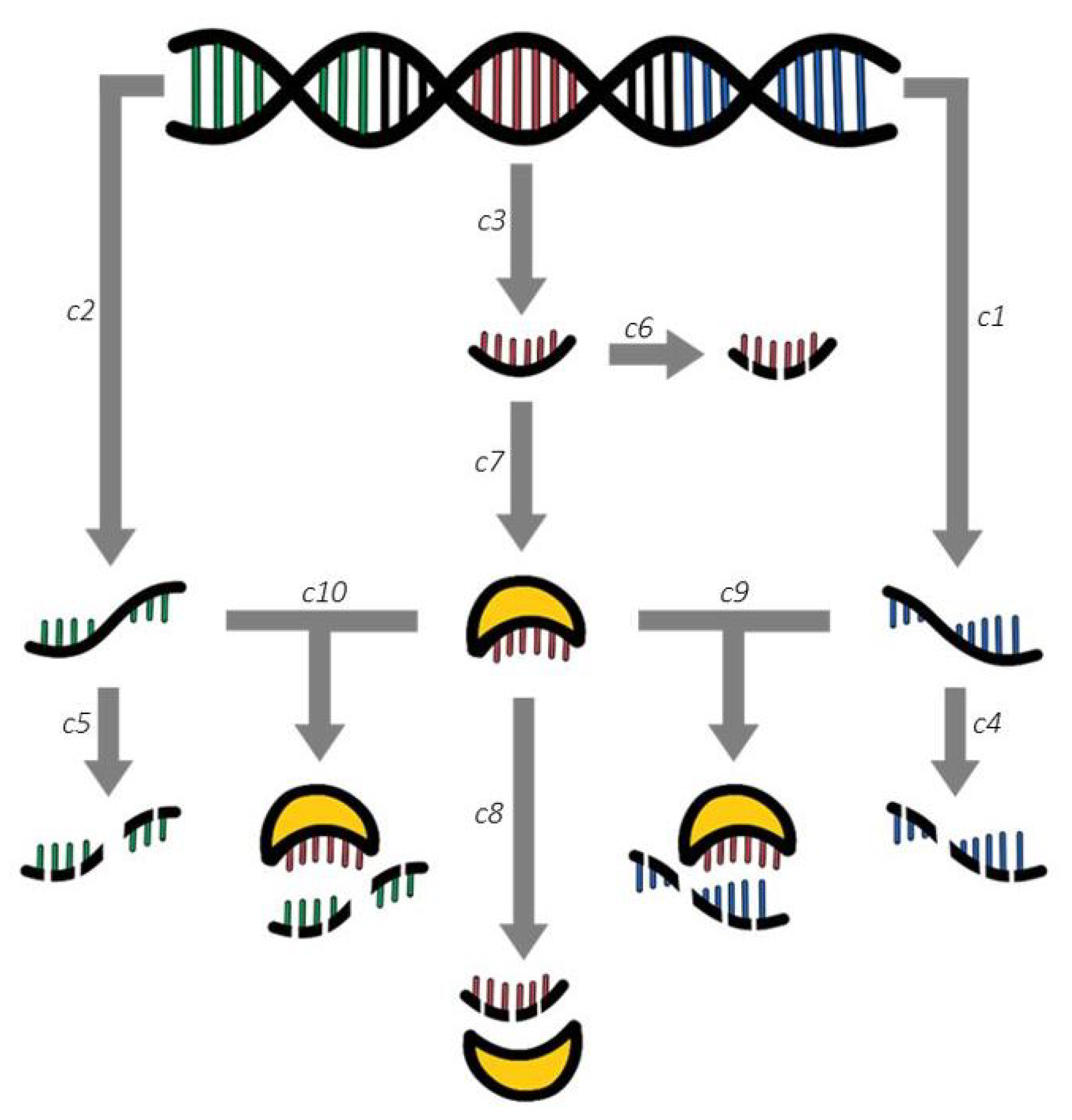
In Figure 1, the double helix symbolizes the DNA sequences attributable to PTEN, miRNAs and ceRNAs, respectively indicated by the vertical bars colored in blue (right helix section), red (middle helix section), green (left section propeller). After their initial transcription in RNA (corresponding to reactions c1, c2, c3), the species can undergo spontaneous degradation within the cell (reactions c4, c5, c6), or they can eventually be translated into a protein, as in the case of the mRNAs of PTEN. For their part, miRNAs can instead be loaded into RISC (reaction c7), thus becoming capable of targeting and degrading both mRNAs and ceRNAs (reactions c9, c10, respectively). This loading also affects the time required for miRNA degradation, which is now higher than for the unloaded miRNAs (reaction c8).

The importance of our new model resides in a few considerations, which we now underline and explain. The first observation concerns the introduction of the loading into RISC as its own reaction, since this process has been repeatedly reported in the literature and referred to as a biological bottleneck: most miRNAs are degraded before such loading can occur, so they lack the ability to bind their targets [11,12].

On the other hand, RISC-loaded miRNAs can persist inside the cell for much longer times [13]; for this reason, a different degradation reaction for loaded miRNAs is provided in our model. To describe the various processes illustrated in Figure 1, our model includes the general set (1a) of chemical kinetic reactions, which represents a blueprint for the further reactions, also present in our model.

$$\begin{array}{ccccccc}\hfill & & {\mathrm{DNA}}_{\mathrm{p}}\hfill & \stackrel{\mathrm{c}1}{⟶}& {\mathrm{RNA}}_{\mathrm{p}}\hfill & +& {\mathrm{DNA}}_{\mathrm{p}}\phantom{movemoretotheleft}\hfill \\ \hfill & & {\mathrm{DNA}}_{{\mathrm{ceRNA}}_{\mathrm{i}}}\hfill & \stackrel{\mathrm{c}2}{⟶}& {\mathrm{ceRNA}}_{\mathrm{i}}\hfill & +& {\mathrm{DNA}}_{{\mathrm{ceRNA}}_{\mathrm{i}}}\hfill \\ \hfill & & {\mathrm{miDNA}}_{\mathrm{j}}\hfill & \stackrel{\mathrm{c}3}{⟶}& {\mathrm{miRNA}}_{\mathrm{j}}\hfill & +& {\mathrm{miDNA}}_{\mathrm{j}}\hfill \\ \hfill & & {\mathrm{RNA}}_{\mathrm{p}}\hfill & \stackrel{\mathrm{c}4}{⟶}& 0\hfill & & \\ \hfill & & {\mathrm{ceRNA}}_{\mathrm{i}}\hfill & \stackrel{\mathrm{c}5}{⟶}& 0\hfill & & \\ \hfill & & {\mathrm{miRNA}}_{\mathrm{j}}\hfill & \stackrel{\mathrm{c}6}{⟶}& 0\hfill & & \\ \hfill & & {\mathrm{miRNA}}_{\mathrm{j}}\hfill & \stackrel{\mathrm{c}7}{⟶}& {\mathrm{lmiRNA}}_{\mathrm{j}}\hfill & & \\ \hfill & & {\mathrm{lmiRNA}}_{\mathrm{j}}\hfill & \stackrel{\mathrm{c}8}{⟶}& 0\hfill & & \\ {\mathrm{lmiRNA}}_{\mathrm{j}}\hfill & +& {\mathrm{RNA}}_{\mathrm{p}}\hfill & \stackrel{\mathrm{c}9}{⟶}& {\mathrm{lmiRNA}}_{\mathrm{j}}\hfill & & \\ {\mathrm{lmiRNA}}_{\mathrm{j}}\hfill & +& {\mathrm{ceRNA}}_{\mathrm{p}}\hfill & \stackrel{\mathrm{c}10}{⟶}& {\mathrm{lmiRNA}}_{\mathrm{j}}\hfill & \end{array}$$

(1a)

The notation adopted in set (1a) is as follows:

• ${\mathrm{DNA}}_{\mathrm{p}}$ is the DNA sequence for PTEN;
• ${\mathrm{RNA}}_{\mathrm{p}}$ is the mRNA of PTEN;
• ${\mathrm{ceRNA}}_{\mathrm{i}}$ is the $\mathrm{i}$-th ceRNA;
• ${\mathrm{DNA}}_{{\mathrm{ceRNA}}_{\mathrm{i}}}$ is the DNA sequence for ${\mathrm{ceRNA}}_{\mathrm{i}};$
• ${\mathrm{miRNA}}_{\mathrm{j}}$ is the $\mathrm{j}$-th miRNA;
• ${\mathrm{miDNA}}_{\mathrm{j}}$ is the DNA sequence for ${\mathrm{miRNA}}_{\mathrm{j}};$
• ${\mathrm{lmiRNA}}_{\mathrm{j}}$ represents the loaded analogue of ${\mathrm{miRNA}}_{\mathrm{j}}.$

Each reaction in (1a) is characterized by a specific coefficient ${\mathrm{c}}_{\mathrm{j}},$ linked to the probability that such a reaction will indeed occur, as well as to the instant of time at which it may occur; notice that the same type of reaction may have a different ${\mathrm{c}}_{\mathrm{j}}$ value (reaction rate) if the interacting species are different. Figure 1 and the related set (1a) display a synthetic version of our model. The complete series of kinetic reactions are in sets (10a)–(10c). Note that the latter represents a simplified deterministic model, in which the instrinsic stochasticity of biochemical reactions is neglected: this allows it to cope with their large number, in addition to the numerous species involved, leading to a high-dimensional differential system, as described below.

A set of ${\mathrm{n}}_{\mathrm{r}}$ monomolecular or bimolecular reactions, the latter having distinct reactants, can be translated into a system of ${\mathrm{n}}_{\mathrm{s}}$ ordinary differential equations (ODEs), where ${\mathrm{n}}_{\mathrm{s}}$ is the total number of $\mathrm{X}$ species that enter the set of chemical reactions and that, within the ODE, assume the role of differential variables ${\mathrm{X}}_1,\dots ,{\mathrm{X}}_{\mathrm{k}},\dots {\mathrm{X}}_{{\mathrm{n}}_{\mathrm{s}}}.$

In other words, ${\mathrm{X}}_{\mathrm{k}}={\mathrm{X}}_{\mathrm{k}}\left(\mathrm{t}\right)$ is a differential variable representing the $\mathrm{k}$-th $\mathrm{X}$-species considered and its biological state at time $\mathrm{t};$ for instance, ${\mathrm{X}}_1$ is ${\mathrm{DNA}}_{\mathrm{p}},$ ${\mathrm{X}}_2$ is ${\mathrm{RNA}}_{\mathrm{p}},$ and so on.

Correspondences between differential variables ${\mathrm{X}}_{\mathrm{k}}$ and the $\mathrm{X}$-species appearing in the small model (1a) are shown in

Table 1. $\mathrm{X}$-species involved in the chemical reactions (1a).

k	${\mathbf{X}}_{\mathbf{k}}$		k	${\mathbf{X}}_{\mathbf{k}}$		k	${\mathbf{X}}_{\mathbf{k}}$		k	${\mathbf{X}}_{\mathbf{k}}$
1	${\mathrm{DNA}}_{\mathrm{p}}$		3	${\mathrm{DNA}}_{{\mathrm{ceRNA}}_{\mathrm{i}}}$		5	${\mathrm{miDNA}}_{\mathrm{j}}$		7	${\mathrm{lmiRNA}}_{\mathrm{j}}$
2	${\mathrm{RNA}}_{\mathrm{p}}$		4	${\mathrm{ceRNA}}_{\mathrm{i}}$		6	${\mathrm{miRNA}}_{\mathrm{j}}$

, through which (1a) itself can be rewritten as (1b).

$$\begin{array}{cccccccccc}{\mathrm{X}}_1\hfill & \stackrel{\mathrm{c}1}{⟶}& {\mathrm{X}}_2\hfill & +& {\mathrm{X}}_1\phantom{separate}\hfill & & & {\mathrm{X}}_6& \stackrel{\mathrm{c}6}{⟶}\hfill & 0\\ {\mathrm{X}}_3\hfill & \stackrel{\mathrm{c}2}{⟶}& {\mathrm{X}}_4\hfill & +& {\mathrm{X}}_3\hfill & & & {\mathrm{X}}_6& \stackrel{\mathrm{c}7}{⟶}\hfill & {\mathrm{X}}_7\\ {\mathrm{X}}_5\hfill & \stackrel{\mathrm{c}3}{⟶}& {\mathrm{X}}_6\hfill & +& {\mathrm{X}}_5\hfill & & & {\mathrm{X}}_7& \stackrel{\mathrm{c}8}{⟶}\hfill & 0\\ {\mathrm{X}}_2\hfill & \stackrel{\mathrm{c}4}{⟶}& 0\hfill & & & {\mathrm{X}}_7& +\hfill & {\mathrm{X}}_2& \stackrel{\mathrm{c}9}{⟶}\hfill & {\mathrm{X}}_7\\ {\mathrm{X}}_4\hfill & \stackrel{\mathrm{c}5}{⟶}& 0\hfill & & & {\mathrm{X}}_7& +\hfill & {\mathrm{X}}_4& \stackrel{\mathrm{c}10}{⟶}\hfill & {\mathrm{X}}_7\end{array}$$

(1b)

In a similar way,

Table 2. $\mathrm{X}$-species involved in the chemical reactions (10a)–(10c).

k	${\mathbf{X}}_{\mathbf{k}}$		k	${\mathbf{X}}_{\mathbf{k}}$		k	${\mathbf{X}}_{\mathbf{k}}$
1	${\mathrm{DNA}}_{\mathrm{p}}$		5	${\mathrm{DNA}}_{\mathrm{VAPA}}$		8	${\mathrm{ceRNA}}_{\mathrm{VAPA}}$
2	${\mathrm{RNA}}_{\mathrm{p}}$		6	${\mathrm{DNA}}_{\mathrm{CNOT}6\mathrm{L}}$		9	${\mathrm{ceRNA}}_{\mathrm{CNOT}6\mathrm{L}}$
3	${\mathrm{miDNA}}_{17}$		7	${\mathrm{DNA}}_{\mathrm{PTENP}1}$		10	${\mathrm{ceRNA}}_{\mathrm{PTENP}1}$
4	${\mathrm{miRNA}}_{17}$					11	${\mathrm{lmiRNA}}_{17}$
12	${\mathrm{miDNA}}_{19\mathrm{a}}$		15	${\mathrm{miRNA}}_{19\mathrm{a}}$		18	${\mathrm{lmiRNA}}_{19\mathrm{a}}$
13	${\mathrm{miDNA}}_{19\mathrm{b}}$		16	${\mathrm{miRNA}}_{19\mathrm{b}}$		19	${\mathrm{lmiRNA}}_{19\mathrm{b}}$
14	${\mathrm{miDNA}}_{214}$		17	${\mathrm{miRNA}}_{214}$		20	${\mathrm{lmiRNA}}_{214}$
21	${\mathrm{miDNA}}_{21}$		27	${\mathrm{miRNA}}_{21}$		33	${\mathrm{lmiRNA}}_{21}$
22	${\mathrm{miDNA}}_{22}$		28	${\mathrm{miRNA}}_{22}$		34	${\mathrm{lmiRNA}}_{22}$
23	${\mathrm{miDNA}}_{25}$		29	${\mathrm{miRNA}}_{25}$		35	${\mathrm{lmiRNA}}_{25}$
24	${\mathrm{miDNA}}_{106}$		30	${\mathrm{miRNA}}_{106}$		36	${\mathrm{lmiRNA}}_{106}$
25	${\mathrm{miDNA}}_{205}$		31	${\mathrm{miRNA}}_{205}$		37	${\mathrm{lmiRNA}}_{205}$
26	${\mathrm{DNA}}_{\mathrm{ZEB}2}$		32	${\mathrm{ceRNA}}_{\mathrm{ZEB}2}$

summarizes the correspondences between differential variables ${\mathrm{X}}_{\mathrm{k}}$ and the $\mathrm{X}$-species considered in the larger simulation presented in Section 3.

The translation from the set of ${\mathrm{n}}_{\mathrm{r}}$ reactions to the system of ${\mathrm{n}}_{\mathrm{s}}$ ordinary differential equations is illustrated in the following, employing model (1b) and its corresponding differential system (7), where the reactions are ${\mathrm{n}}_{\mathrm{r}}=10$ and the differential equations are ${\mathrm{n}}_{\mathrm{s}}=7.$

Formula (2) provides the general form of the ODE $\mathrm{k}$-th representative, for $\mathrm{k}=1,\dots ,{\mathrm{n}}_{\mathrm{s}}.$

$${\displaystyle {\mathrm{X}}_{\mathrm{k}}^{\prime }\left(\mathrm{t}\right)=\sum _{\mathrm{j}=1}^{{\mathrm{n}}_{\mathrm{r}}}{\nu }_{\mathrm{k}\mathrm{j}}{\mathrm{c}}_{\mathrm{j}}{\mathcal{X}}_{\mathrm{j}}\left(\mathrm{t}\right),{\mathcal{X}}_j\left(t\right)=\left\{\begin{array}{cc}{\mathrm{X}}_{\mathrm{p}}\left(\mathrm{t}\right)\hfill & \mathrm{reaction\; j\; monomolecular},\hfill \\ {\mathrm{X}}_{\mathrm{p}}\left(\mathrm{t}\right){\mathrm{X}}_{\mathrm{q}}\left(\mathrm{t}\right)\hfill & \mathrm{reaction\; j\; bimolecular}.\hfill \end{array}\right.}$$

(2)

The differential variables ${\mathrm{X}}_{\mathrm{p}}$ and ${\mathrm{X}}_{\mathrm{q}},$ with $\mathrm{p},\mathrm{q}\in \{1,\dots ,{\mathrm{n}}_{\mathrm{s}}\},$ are the reactants appearing in the $\mathrm{j}$-th reaction, whose reaction rate is ${\mathrm{c}}_{\mathrm{j}}.$ The role of the scalar quantities ${\nu }_{\mathrm{k}\mathrm{j}}$ is introduced shortly.

As an example, the second $(\mathrm{k}=2)$ differential equation in (7) is:

$${\mathrm{X}}_{{\mathrm{k}|}_{\mathrm{k}=2}}^{\prime }={\nu }_{2,1}{\mathrm{c}}_1{\mathrm{X}}_1+{\nu }_{2,4}{\mathrm{c}}_4{\mathrm{X}}_2+{\nu }_{2,9}{\mathrm{c}}_9{\mathrm{X}}_7{\mathrm{X}}_2,$$

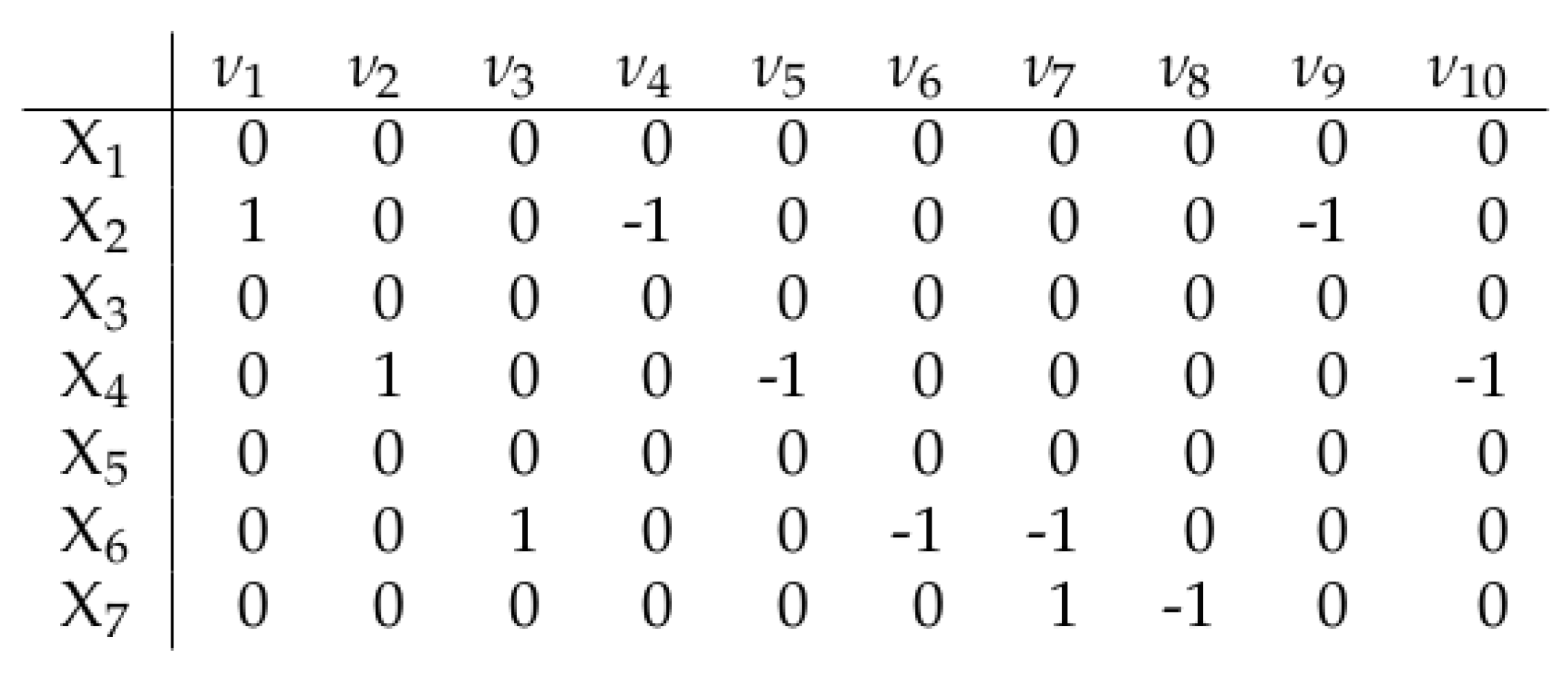
since ${\nu }_{2,2}={\nu }_{2,3}={\nu }_{2,5}={\nu }_{2,6}={\nu }_{2,7}={\nu }_{2,8}={\nu }_{2,10}=0$ (see row 2 of Figure 2), which indicates that the reactions of (1b) contributing to the definition of ${\mathrm{X}}_{{\mathrm{k}|}_{\mathrm{k}=2}}^{\prime }$ are the first, fourth and ninth ones, whose reactants are, respectively: ${\mathrm{X}}_1$ in reaction ${\mathrm{c}}_1;$ ${\mathrm{X}}_2$ in reaction ${\mathrm{c}}_4;$ the pair ${\mathrm{X}}_7,{\mathrm{X}}_2$ in reaction ${\mathrm{c}}_9.$ Indeed, this mirrors the fact that ${\mathrm{X}}_{{\mathrm{k}|}_{\mathrm{k}=2}}$ appears (as a reactant or product or both) only in the first, fourth and ninth reactions of (1b).

The scalar quantities ${\nu }_{\mathrm{k}\mathrm{j}}$ in (3) are in fact related to the stoichiometry of the chemical reactions. They are collected column-wise to form the so-called stoichiometric vectors ${\nu }_{\mathrm{j}},$ with $\mathrm{j}=1,\dots ,{\mathrm{n}}_{\mathrm{r}}.$ For each $\mathrm{j}$-th reaction, the correspondent ${\nu }_{\mathrm{j}}$ is defined as in (4).

$${\nu }_{\mathrm{j}}={\left({\nu }_{1\mathrm{j}},\dots ,{\nu }_{\mathrm{k}\mathrm{j}},\dots ,{\nu }_{{\mathrm{n}}_{\mathrm{s}}\mathrm{j}}\right)}^{\mathrm{T}},{\nu }_{\mathrm{k}\mathrm{j}}=\left\{\begin{array}{cc}-1\hfill & \mathrm{if}{\mathrm{X}}_{\mathrm{k}}\mathrm{is\; a\; reactant};\hfill \\ 0\hfill & \mathrm{if}{\mathrm{X}}_{\mathrm{k}}\mathrm{is\; not\; involved};\hfill \\ 1\hfill & \mathrm{if}{\mathrm{X}}_{\mathrm{k}}\mathrm{is\; a\; product}.\hfill \end{array}\right.$$

(3)

Notice that if ${\mathrm{X}}_{\mathrm{k}}$ is both a reactant and a product in the $\mathrm{j}$-th reaction, then it is obviously ${\nu }_{\mathrm{k}\mathrm{j}}=-1+1=0.$

A stoichiometric matrix $\mathrm{S}=\left({\nu }_{\mathrm{k}\mathrm{j}}\right)$ of dimensions ${\mathrm{n}}_{\mathrm{s}}\times {\mathrm{n}}_{\mathrm{r}}$ can thus be defined; for instance, in the case of set (1b), $\mathrm{S}$ takes the form outlined in Figure 2.

The notation in (2) can be simplified by introducing the so-called propensity functions, whose $\mathrm{j}$-th entry takes the general form (4), where $\mathrm{p},\mathrm{q}\in \{1,\dots ,{\mathrm{n}}_{\mathrm{s}}\}$ and $\mathrm{j}=1,\dots ,{\mathrm{n}}_{\mathrm{r}}.$

$${\mathrm{a}}_{\mathrm{j}}\left(\mathrm{t}\right)={\mathrm{c}}_{\mathrm{j}}{\mathcal{X}}_{\mathrm{j}}\left(\mathrm{t}\right),{\mathcal{X}}_j\left(t\right)=\left\{\begin{array}{cc}{\mathrm{X}}_{\mathrm{p}}\left(\mathrm{t}\right)\hfill & \mathrm{reaction\; j\; monomolecular},\hfill \\ {\mathrm{X}}_{\mathrm{p}}\left(\mathrm{t}\right){\mathrm{X}}_{\mathrm{q}}\left(\mathrm{t}\right)\hfill & \mathrm{reaction\; j\; bimolecular}.\hfill \end{array}\right.$$

(4)

For each $\mathrm{j}$-th reaction, ${\mathrm{a}}_{\mathrm{j}}\left(\mathrm{t}\right)$ expresses the link between the probability ${\mathrm{c}}_{\mathrm{j}}$ and the reactants involved; for instance, the propensity functions corresponding to (1b) are shown in (5), where dependence on time $\mathrm{t}$ has been temporarily discarded, to ease the notation.

$$\begin{array}{cccccc}{\mathrm{a}}_1\hfill & =& {\mathrm{c}}_1{\mathrm{X}}_1,\phantom{separate}\hfill & {\mathrm{a}}_6\hfill & =& {\mathrm{c}}_6{\mathrm{X}}_6,\hfill \\ {\mathrm{a}}_2\hfill & =& {\mathrm{c}}_2{\mathrm{X}}_3,\hfill & {\mathrm{a}}_7\hfill & =& {\mathrm{c}}_7{\mathrm{X}}_6,\hfill \\ {\mathrm{a}}_3\hfill & =& {\mathrm{c}}_3{\mathrm{X}}_5,\hfill & {\mathrm{a}}_8\hfill & =& {\mathrm{c}}_8{\mathrm{X}}_7,\hfill \\ {\mathrm{a}}_4\hfill & =& {\mathrm{c}}_4{\mathrm{X}}_2,\hfill & {\mathrm{a}}_9\hfill & =& {\mathrm{c}}_9{\mathrm{X}}_7{\mathrm{X}}_2,\hfill \\ {\mathrm{a}}_5\hfill & =& {\mathrm{c}}_5{\mathrm{X}}_4,\hfill & {\mathrm{a}}_{10}\hfill & =& {\mathrm{c}}_{10}{\mathrm{X}}_7{\mathrm{X}}_4.\hfill \end{array}$$

(5)

The ODE system can then be written in matrix form:

$${\mathrm{X}}^{\prime }\left(\mathrm{t}\right)=\mathrm{S}\mathrm{a}\left(\mathrm{t}\right),$$

(6)

where:

$$\begin{array}{cc}\hfill {\mathrm{X}}^{\prime }\left(\mathrm{t}\right)& ={\left({\mathrm{X}}_1^{\prime }\left(\mathrm{t}\right),\dots ,{\mathrm{X}}_{\mathrm{k}}^{\prime }\left(\mathrm{t}\right),\dots ,{\mathrm{X}}_{{\mathrm{n}}_{\mathrm{s}}}^{\prime }\left(\mathrm{t}\right)\right)}^{\mathrm{T}},\hfill \\ \hfill \mathrm{a}\left(\mathrm{t}\right)& ={\left({\mathrm{a}}_1\left(\mathrm{t}\right),\dots \dots ,{\mathrm{a}}_{\mathrm{j}}\left(\mathrm{t}\right),\dots \dots ,{\mathrm{a}}_{{\mathrm{n}}_{\mathrm{r}}}\left(\mathrm{t}\right)\right)}^{\mathrm{T}}.\hfill \end{array}$$

The system dimensions obviously depend on the number ${\mathrm{n}}_{\mathrm{s}}$ of $\mathrm{X}$-species involved (i.e., number of differential equations) and the number ${\mathrm{n}}_{\mathrm{r}}$ of reactions considered (i.e., number of parameters). The ODE system for model (1b) is as in (7), with seven equations and ten parameters, and where again dependence on time $\mathrm{t}$ has been temporarily discarded.

$$\begin{array}{ccccc}{\mathrm{X}}_1^{\prime }\hfill & =& 0\hfill & & \\ {\mathrm{X}}_2^{\prime }\hfill & =& {\mathrm{a}}_1-{\mathrm{a}}_4-{\mathrm{a}}_9\hfill & =& {\mathrm{c}}_1{\mathrm{X}}_1-{\mathrm{c}}_4{\mathrm{X}}_2-{\mathrm{c}}_9{\mathrm{X}}_7{\mathrm{X}}_2\hfill \\ {\mathrm{X}}_3^{\prime }\hfill & =& 0\hfill & & \\ {\mathrm{X}}_4^{\prime }\hfill & =& {\mathrm{a}}_2-{\mathrm{a}}_5-{\mathrm{a}}_{10}\hfill & =& {\mathrm{c}}_2{\mathrm{X}}_3-{\mathrm{c}}_5{\mathrm{X}}_4-{\mathrm{c}}_{10}{\mathrm{X}}_7{\mathrm{X}}_4\hfill \\ {\mathrm{X}}_5^{\prime }\hfill & =& 0\hfill & & \\ {\mathrm{X}}_6^{\prime }\hfill & =& {\mathrm{a}}_3-{\mathrm{a}}_6-{\mathrm{a}}_7\hfill & =& {\mathrm{c}}_3{\mathrm{X}}_5-{\mathrm{c}}_6{\mathrm{X}}_6-{\mathrm{c}}_7{\mathrm{X}}_6\hfill \\ {\mathrm{X}}_7^{\prime }\hfill & =& {\mathrm{a}}_7-{\mathrm{a}}_8\hfill & =& {\mathrm{c}}_7{\mathrm{X}}_6-{\mathrm{c}}_8{\mathrm{X}}_7\hfill \end{array}$$

(7)

By defining initial conditions at time $\mathrm{t}={\mathrm{T}}_0:$

$${\mathrm{X}}_{\mathrm{k}}\left({\mathrm{T}}_0\right)={\mathrm{X}}_{\mathrm{k},0}\mathrm{k}=1,\dots ,{\mathrm{n}}_{\mathrm{s}},$$

(8)

the ODE (6) becomes an Initial Value Problem (IVP), whose integration over the time interval $[{\mathrm{T}}_0,\mathrm{T}]$ will yield the solution vector (or state vector):

$$\mathrm{X}\left(\mathrm{t}\right)={\left({\mathrm{X}}_1\left(\mathrm{t}\right),\dots ,{\mathrm{X}}_{\mathrm{k}}\left(\mathrm{t}\right),\dots ,{\mathrm{X}}_{{\mathrm{n}}_{\mathrm{s}}}\left(\mathrm{t}\right)\right)}^{\mathrm{T}}.$$

(9)

3. Simulation

In this section, a complete set of chemical reactions is presented, grouped into three subsets (10a)–(10c) for readability.

Table 2 reports all the $\mathrm{X}$-species considered in such subsets, as well as their correspondences with the differential variables ${\mathrm{X}}_{\mathrm{k}},$ which are as follows: the first sixteen reactions in (10a) involve ${\mathrm{X}}_1$ to ${\mathrm{X}}_{11};$ the next twenty (from 17 to 36) reactions in (10b) involve ${\mathrm{X}}_{12}$ to ${\mathrm{X}}_{20},$ as well as some among ${\mathrm{X}}_1$ to ${\mathrm{X}}_{11};$ finally, the last thirty-one (from 37 to 67) reactions in (10c) involve ${\mathrm{X}}_{21}$ to ${\mathrm{X}}_{37},$ and again some among ${\mathrm{X}}_1$ to ${\mathrm{X}}_{11}.$

$$\begin{array}{ccccccc}\hfill & & {\mathrm{DNA}}_{\mathrm{p}}\hfill & \stackrel{\mathrm{c}1}{⟶}& {\mathrm{RNA}}_{\mathrm{p}}\hfill & +& {\mathrm{DNA}}_{\mathrm{p}}\phantom{movetoleft}\hfill \\ \hfill & & {\mathrm{RNA}}_{\mathrm{p}}\hfill & \stackrel{\mathrm{c}2}{⟶}& 0\hfill & & \\ \hfill & & {\mathrm{miDNA}}_{17}\hfill & \stackrel{\mathrm{c}3}{⟶}& {\mathrm{miRNA}}_{17}\hfill & +& {\mathrm{miDNA}}_{17}\hfill \\ \hfill & & {\mathrm{miRNA}}_{17}\hfill & \stackrel{\mathrm{c}4}{⟶}& 0\hfill & & \\ \hfill & & {\mathrm{DNA}}_{\mathrm{VAPA}}\hfill & \stackrel{\mathrm{c}5}{⟶}& {\mathrm{ceRNA}}_{\mathrm{VAPA}}\hfill & +& {\mathrm{DNA}}_{\mathrm{VAPA}}\hfill \\ \hfill & & {\mathrm{DNA}}_{\mathrm{CNOT}6\mathrm{L}}\hfill & \stackrel{\mathrm{c}6}{⟶}& {\mathrm{ceRNA}}_{\mathrm{CNOT}6\mathrm{L}}\hfill & +& {\mathrm{DNA}}_{\mathrm{CNOT}6\mathrm{L}}\hfill \\ \hfill & & {\mathrm{DNA}}_{\mathrm{PTENP}1}\hfill & \stackrel{\mathrm{c}7}{⟶}& {\mathrm{ceRNA}}_{\mathrm{PTENP}1}\hfill & +& {\mathrm{DNA}}_{\mathrm{PTENP}1}\hfill \\ \hfill & & {\mathrm{ceRNA}}_{\mathrm{VAPA}}\hfill & \stackrel{\mathrm{c}8}{⟶}& 0\hfill & & \\ \hfill & & {\mathrm{ceRNA}}_{\mathrm{CNOT}6\mathrm{L}}\hfill & \stackrel{\mathrm{c}9}{⟶}& 0\hfill & & \\ \hfill & & {\mathrm{ceRNA}}_{\mathrm{PTENP}1}\hfill & \stackrel{\mathrm{c}10}{⟶}& 0\hfill & & \\ \hfill & & {\mathrm{miRNA}}_{17}\hfill & \stackrel{\mathrm{c}11}{⟶}& {\mathrm{lmiRNA}}_{17}\hfill & & \\ {\mathrm{lmiRNA}}_{17}\hfill & +& {\mathrm{RNA}}_{\mathrm{p}}\hfill & \stackrel{\mathrm{c}12}{⟶}& {\mathrm{lmiRNA}}_{17}\hfill & & \\ {\mathrm{lmiRNA}}_{17}\hfill & +& {\mathrm{ceRNA}}_{\mathrm{VAPA}}\hfill & \stackrel{\mathrm{c}13}{⟶}& {\mathrm{lmiRNA}}_{17}\hfill & & \\ {\mathrm{lmiRNA}}_{17}\hfill & +& {\mathrm{ceRNA}}_{\mathrm{CNOT}6\mathrm{L}}\hfill & \stackrel{\mathrm{c}14}{⟶}& {\mathrm{lmiRNA}}_{17}\hfill & & \\ {\mathrm{lmiRNA}}_{17}\hfill & +& {\mathrm{ceRNA}}_{\mathrm{PTENP}1}\hfill & \stackrel{\mathrm{c}15}{⟶}& {\mathrm{lmiRNA}}_{17}\hfill & & \\ \hfill & & {\mathrm{lmiRNA}}_{17}\hfill & \stackrel{\mathrm{c}16}{⟶}& 0\hfill & & \end{array}$$

(10a)

$$\begin{array}{ccccccc}\hfill & & {\mathrm{miDNA}}_{19\mathrm{a}}\hfill & \stackrel{\mathrm{c}17}{⟶}& {\mathrm{miRNA}}_{19\mathrm{a}}\hfill & +& {\mathrm{miDNA}}_{19\mathrm{a}}\phantom{moveleft}\hfill \\ \hfill & & {\mathrm{miDNA}}_{19\mathrm{b}}\hfill & \stackrel{\mathrm{c}18}{⟶}& {\mathrm{miRNA}}_{19\mathrm{b}}\hfill & +& {\mathrm{miDNA}}_{19\mathrm{b}}\hfill \\ \hfill & & {\mathrm{miDNA}}_{214}\hfill & \stackrel{\mathrm{c}19}{⟶}& {\mathrm{miRNA}}_{214}\hfill & +& {\mathrm{miDNA}}_{214}\hfill \\ \hfill & & {\mathrm{miRNA}}_{19\mathrm{a}}\hfill & \stackrel{\mathrm{c}20}{⟶}& 0\hfill & & \\ \hfill & & {\mathrm{miRNA}}_{19\mathrm{b}}\hfill & \stackrel{\mathrm{c}21}{⟶}& 0\hfill & & \\ \hfill & & {\mathrm{miRNA}}_{214}\hfill & \stackrel{\mathrm{c}22}{⟶}& 0\hfill & & \\ \hfill & & {\mathrm{miRNA}}_{19\mathrm{a}}\hfill & \stackrel{\mathrm{c}23}{⟶}& {\mathrm{lmiRNA}}_{19\mathrm{a}}\hfill & & \\ \hfill & & {\mathrm{miRNA}}_{19\mathrm{b}}\hfill & \stackrel{\mathrm{c}24}{⟶}& {\mathrm{lmiRNA}}_{19\mathrm{b}}\hfill & & \\ \hfill & & {\mathrm{miRNA}}_{214}\hfill & \stackrel{\mathrm{c}25}{⟶}& {\mathrm{lmiRNA}}_{214}\hfill & & \\ \hfill & & {\mathrm{lmiRNA}}_{19\mathrm{a}}\hfill & \stackrel{\mathrm{c}26}{⟶}& 0\hfill & & \\ \hfill & & {\mathrm{lmiRNA}}_{19\mathrm{b}}\hfill & \stackrel{\mathrm{c}27}{⟶}& 0\hfill & & \\ \hfill & & {\mathrm{lmiRNA}}_{214}\hfill & \stackrel{\mathrm{c}28}{⟶}& 0\hfill & & \\ {\mathrm{lmiRNA}}_{19\mathrm{a}}\hfill & +& {\mathrm{RNA}}_{\mathrm{p}}\hfill & \stackrel{\mathrm{c}29}{⟶}& {\mathrm{lmiRNA}}_{19\mathrm{a}}\hfill & & \\ {\mathrm{lmiRNA}}_{19\mathrm{b}}\hfill & +& {\mathrm{RNA}}_{\mathrm{p}}\hfill & \stackrel{\mathrm{c}30}{⟶}& {\mathrm{lmiRNA}}_{19\mathrm{b}}\hfill & & \\ {\mathrm{lmiRNA}}_{214}\hfill & +& {\mathrm{RNA}}_{\mathrm{p}}\hfill & \stackrel{\mathrm{c}31}{⟶}& {\mathrm{lmiRNA}}_{214}\hfill & & \\ {\mathrm{lmiRNA}}_{19\mathrm{b}}\hfill & +& {\mathrm{ceRNA}}_{\mathrm{PTENP}1}\hfill & \stackrel{\mathrm{c}32}{⟶}& {\mathrm{lmiRNA}}_{19\mathrm{b}}\hfill & & \\ {\mathrm{lmiRNA}}_{214}\hfill & +& {\mathrm{ceRNA}}_{\mathrm{PTENP}1}\hfill & \stackrel{\mathrm{c}33}{⟶}& {\mathrm{lmiRNA}}_{214}\hfill & & \\ {\mathrm{lmiRNA}}_{19\mathrm{a}}\hfill & +& {\mathrm{ceRNA}}_{\mathrm{VAPA}}\hfill & \stackrel{\mathrm{c}34}{⟶}& {\mathrm{lmiRNA}}_{19\mathrm{a}}\hfill & & \\ {\mathrm{lmiRNA}}_{19\mathrm{a}}\hfill & +& {\mathrm{ceRNA}}_{\mathrm{CNOT}6\mathrm{L}}\hfill & \stackrel{\mathrm{c}35}{⟶}& {\mathrm{lmiRNA}}_{19\mathrm{a}}\hfill & & \\ {\mathrm{lmiRNA}}_{19\mathrm{b}}\hfill & +& {\mathrm{ceRNA}}_{\mathrm{CNOT}6\mathrm{L}}\hfill & \stackrel{\mathrm{c}36}{⟶}& {\mathrm{lmiRNA}}_{19\mathrm{b}}\hfill & \end{array}$$

(10b)

$$\begin{array}{ccccccc}\hfill & & {\mathrm{miDNA}}_{21}\hfill & \stackrel{\mathrm{c}37}{⟶}& {\mathrm{miRNA}}_{21}\hfill & +& {\mathrm{miDNA}}_{21}\hfill \\ \hfill & & {\mathrm{miDNA}}_{22}\hfill & \stackrel{\mathrm{c}38}{⟶}& {\mathrm{miRNA}}_{22}\hfill & +& {\mathrm{miDNA}}_{22}\hfill \\ \hfill & & {\mathrm{miDNA}}_{25}\hfill & \stackrel{\mathrm{c}39}{⟶}& {\mathrm{miRNA}}_{25}\hfill & +& {\mathrm{miDNA}}_{25}\hfill \\ \hfill & & {\mathrm{miDNA}}_{106}\hfill & \stackrel{\mathrm{c}40}{⟶}& {\mathrm{miRNA}}_{106}\hfill & +& {\mathrm{miDNA}}_{106}\hfill \\ \hfill & & {\mathrm{miDNA}}_{205}\hfill & \stackrel{\mathrm{c}41}{⟶}& {\mathrm{miRNA}}_{205}\hfill & +& {\mathrm{miDNA}}_{205}\hfill \\ \hfill & & {\mathrm{DNA}}_{\mathrm{ZEB}2}\hfill & \stackrel{\mathrm{c}42}{⟶}& {\mathrm{ceRNA}}_{\mathrm{ZEB}2}\hfill & +& {\mathrm{DNA}}_{\mathrm{ZEB}2}\hfill \\ \hfill & & {\mathrm{miRNA}}_{21}\hfill & \stackrel{\mathrm{c}43}{⟶}& 0\hfill & & \\ \hfill & & {\mathrm{miRNA}}_{22}\hfill & \stackrel{\mathrm{c}44}{⟶}& 0\hfill & & \\ \hfill & & {\mathrm{miRNA}}_{25}\hfill & \stackrel{\mathrm{c}45}{⟶}& 0\hfill & & \\ \hfill & & {\mathrm{miRNA}}_{106}\hfill & \stackrel{\mathrm{c}46}{⟶}& 0\hfill & & \\ \hfill & & {\mathrm{miRNA}}_{205}\hfill & \stackrel{\mathrm{c}47}{⟶}& 0\hfill & & \\ \hfill & & {\mathrm{ceRNA}}_{\mathrm{ZEB}2}\hfill & \stackrel{\mathrm{c}48}{⟶}& 0\hfill & & \\ \hfill & & {\mathrm{miRNA}}_{21}\hfill & \stackrel{\mathrm{c}49}{⟶}& {\mathrm{lmiRNA}}_{21}\hfill & & \\ \hfill & & {\mathrm{miRNA}}_{22}\hfill & \stackrel{\mathrm{c}50}{⟶}& {\mathrm{lmiRNA}}_{22}\hfill & & \\ \hfill & & {\mathrm{miRNA}}_{25}\hfill & \stackrel{\mathrm{c}51}{⟶}& {\mathrm{lmiRNA}}_{25}\hfill & & \\ \hfill & & {\mathrm{miRNA}}_{106}\hfill & \stackrel{\mathrm{c}52}{⟶}& {\mathrm{lmiRNA}}_{106}\hfill & & \\ \hfill & & {\mathrm{miRNA}}_{205}\hfill & \stackrel{\mathrm{c}53}{⟶}& {\mathrm{lmiRNA}}_{205}\hfill & & \\ {\mathrm{lmiRNA}}_{21}\hfill & +& {\mathrm{RNA}}_{\mathrm{p}}\hfill & \stackrel{\mathrm{c}54}{⟶}& {\mathrm{lmiRNA}}_{21}\hfill & & \\ {\mathrm{lmiRNA}}_{22}\hfill & +& {\mathrm{RNA}}_{\mathrm{p}}\hfill & \stackrel{\mathrm{c}55}{⟶}& {\mathrm{lmiRNA}}_{22}\hfill & & \\ {\mathrm{lmiRNA}}_{25}\hfill & +& {\mathrm{RNA}}_{\mathrm{p}}\hfill & \stackrel{\mathrm{c}56}{⟶}& {\mathrm{lmiRNA}}_{25}\hfill & & \\ {\mathrm{lmiRNA}}_{106}\hfill & +& {\mathrm{RNA}}_{\mathrm{p}}\hfill & \stackrel{\mathrm{c}57}{⟶}& {\mathrm{lmiRNA}}_{106}\hfill & & \\ {\mathrm{lmiRNA}}_{205}\hfill & +& {\mathrm{RNA}}_{\mathrm{p}}\hfill & \stackrel{\mathrm{c}58}{⟶}& {\mathrm{lmiRNA}}_{205}\hfill & & \\ {\mathrm{lmiRNA}}_{106}\hfill & +& {\mathrm{ceRNA}}_{\mathrm{VAPA}}\hfill & \stackrel{\mathrm{c}59}{⟶}& {\mathrm{lmiRNA}}_{106}\hfill & & \\ {\mathrm{lmiRNA}}_{106}\hfill & +& {\mathrm{ceRNA}}_{\mathrm{CNOT}6\mathrm{L}}\hfill & \stackrel{\mathrm{c}60}{⟶}& {\mathrm{lmiRNA}}_{106}\hfill & & \\ {\mathrm{lmiRNA}}_{21}\hfill & +& {\mathrm{ceRNA}}_{\mathrm{PTENP}1}\hfill & \stackrel{\mathrm{c}61}{⟶}& {\mathrm{lmiRNA}}_{21}\hfill & & \\ {\mathrm{lmiRNA}}_{25}\hfill & +& {\mathrm{ceRNA}}_{\mathrm{ZEB}2}\hfill & \stackrel{\mathrm{c}62}{⟶}& {\mathrm{lmiRNA}}_{25}\hfill & & \\ \hfill & & {\mathrm{lmiRNA}}_{21}\hfill & \stackrel{\mathrm{c}63}{⟶}& 0\hfill & & \\ \hfill & & {\mathrm{lmiRNA}}_{22}\hfill & \stackrel{\mathrm{c}64}{⟶}& 0\hfill & & \\ \hfill & & {\mathrm{lmiRNA}}_{25}\hfill & \stackrel{\mathrm{c}65}{⟶}& 0\hfill & & \\ \hfill & & {\mathrm{lmiRNA}}_{106}\hfill & \stackrel{\mathrm{c}66}{⟶}& 0\hfill & & \\ \hfill & & {\mathrm{lmiRNA}}_{205}\hfill & \stackrel{\mathrm{c}67}{⟶}& 0\hfill & \end{array}$$

(10c)

Reactions (10a)–(10c) can then be rewritten in differential form: although their explicit translation in terms of ${\mathrm{X}}_{\mathrm{k}}$ is not provided here, the procedure to obtain the correspondent ODE system is the same as that described in Section 2 for the small model (1a).

The stoichiometric matrix $\mathrm{S}=\left({\nu }_{\mathrm{k}\mathrm{j}}\right)$ associated with (10a)–(10c) has dimensions $37\times 67$ and elements given by (3).

As for the propensity functions related to (10a)–(10c), they are listed in (11), where we set ${\mathrm{a}}_{\mathrm{j}}={\mathrm{a}}_{\mathrm{j}}\left(\mathrm{t}\right)$ and ${\mathrm{X}}_{\mathrm{k}}={\mathrm{X}}_{\mathrm{k}}\left(\mathrm{t}\right)$ for brevity.

$$\begin{array}{ccccccc}{\mathrm{a}}_{\mathrm{j}}\hfill & =& {\mathrm{c}}_{\mathrm{j}}\hfill & {\mathrm{X}}_{\mathrm{j}}\hfill & \hfill & \phantom{movetoleft-5}& \mathrm{j}=1,\dots ,10,\hfill \\ {\mathrm{a}}_{11}\hfill & =& {\mathrm{c}}_{11}\hfill & {\mathrm{X}}_4\hfill & \hfill & & \\ {\mathrm{a}}_{12}\hfill & =& {\mathrm{c}}_{12}\hfill & {\mathrm{X}}_2\hfill & {\mathrm{X}}_{11}\hfill & & \\ {\mathrm{a}}_{\mathrm{j}}\hfill & =& {\mathrm{c}}_{\mathrm{j}}\hfill & {\mathrm{X}}_{\mathrm{j}-5}\hfill & {\mathrm{X}}_{11}\hfill & & \mathrm{j}=13,\dots ,15,\hfill \\ {\mathrm{a}}_{16}\hfill & =& {\mathrm{c}}_{16}\hfill & {\mathrm{X}}_{11}\hfill & \hfill & & \\ \\ {\mathrm{a}}_{\mathrm{j}}\hfill & =& {\mathrm{c}}_{\mathrm{j}}\hfill & {\mathrm{X}}_{\mathrm{j}-5}\hfill & \hfill & \phantom{movetoleft}& \mathrm{j}=17,\dots ,22,\hfill \\ {\mathrm{a}}_{\mathrm{j}}\hfill & =& {\mathrm{c}}_{\mathrm{j}}\hfill & {\mathrm{X}}_{\mathrm{j}-8}\hfill & \hfill & & \mathrm{j}=23,\dots ,28,\hfill \\ {\mathrm{a}}_{\mathrm{j}}\hfill & =& {\mathrm{c}}_{\mathrm{j}}\hfill & {\mathrm{X}}_2\hfill & {\mathrm{X}}_{\mathrm{j}-11}\hfill & & \mathrm{j}=29,\dots ,31,\hfill \\ {\mathrm{a}}_{\mathrm{j}}\hfill & =& {\mathrm{c}}_{\mathrm{j}}\hfill & {\mathrm{X}}_{10}\hfill & {\mathrm{X}}_{\mathrm{j}-13}\hfill & & \mathrm{j}=32,33,\hfill \\ {\mathrm{a}}_{34}\hfill & =& {\mathrm{c}}_{34}\hfill & {\mathrm{X}}_8\hfill & {\mathrm{X}}_{18}\hfill & & \\ {\mathrm{a}}_{\mathrm{j}}\hfill & =& {\mathrm{c}}_{\mathrm{j}}\hfill & {\mathrm{X}}_9\hfill & {\mathrm{X}}_{\mathrm{j}-17}\hfill & & \mathrm{j}=35,36,\hfill \\ \\ {\mathrm{a}}_{\mathrm{j}}\hfill & =& {\mathrm{c}}_{\mathrm{j}}\hfill & {\mathrm{X}}_{\mathrm{j}-16}\hfill & \hfill & \phantom{movetoleft}& \mathrm{j}=37,\dots ,48,\hfill \\ {\mathrm{a}}_{\mathrm{j}}\hfill & =& {\mathrm{c}}_{\mathrm{j}}\hfill & {\mathrm{X}}_{\mathrm{j}-22}\hfill & \hfill & & \mathrm{j}=49,\dots ,53,\hfill \\ {\mathrm{a}}_{\mathrm{j}}\hfill & =& {\mathrm{c}}_{\mathrm{j}}\hfill & {\mathrm{X}}_2\hfill & {\mathrm{X}}_{\mathrm{j}-21}\hfill & & \mathrm{j}=54,\dots ,58,\hfill \\ {\mathrm{a}}_{\mathrm{j}}\hfill & =& {\mathrm{c}}_{\mathrm{j}}\hfill & {\mathrm{X}}_{36}\hfill & {\mathrm{X}}_{\mathrm{j}-51}\hfill & & \mathrm{j}=59,60,\hfill \\ {\mathrm{a}}_{61}\hfill & =& {\mathrm{c}}_{61}\hfill & {\mathrm{X}}_{10}\hfill & {\mathrm{X}}_{33}\hfill & & \\ {\mathrm{a}}_{62}\hfill & =& {\mathrm{c}}_{62}\hfill & {\mathrm{X}}_{32}\hfill & {\mathrm{X}}_{35}\hfill & & \\ {\mathrm{a}}_{\mathrm{j}}\hfill & =& {\mathrm{c}}_{\mathrm{j}}\hfill & {\mathrm{X}}_{\mathrm{j}-30}\hfill & \hfill & & \mathrm{j}=63,\dots ,67.\hfill \end{array}$$

(11)

Given the propensity functions (11) and the $37\times 67$ stoichiometric matrix $\mathrm{S},$ with entries given by Formula (3) applied to reactions (10a)–(10c), the ODE system that we consider has thirty-seven equations and sixty-seven parameters and takes the form shown in (12), where, again, time dependence has been discarded for brevity.

$$\begin{array}{ccc}{\mathrm{X}}_1^{\prime }\hfill & =& 0\hfill \\ {\mathrm{X}}_2^{\prime }\hfill & =& {\mathrm{a}}_1-{\mathrm{a}}_2-{\mathrm{a}}_{12}-{\mathrm{a}}_{29}-{\mathrm{a}}_{30}-{\mathrm{a}}_{31}-{\mathrm{a}}_{54}-{\mathrm{a}}_{55}-{\mathrm{a}}_{56}-{\mathrm{a}}_{57}-{\mathrm{a}}_{58}\hfill \\ {\mathrm{X}}_3^{\prime }\hfill & =& 0\hfill \\ {\mathrm{X}}_4^{\prime }\hfill & =& {\mathrm{a}}_3-{\mathrm{a}}_4-{\mathrm{a}}_{11}\hfill \\ {\mathrm{X}}_{\mathrm{k}}^{\prime }\hfill & =& 0\phantom{{\mathrm{a}}_{12}-{\mathrm{a}}_{29}-{\mathrm{a}}_{30}-{\mathrm{a}}_{31}-{\mathrm{a}}_{54}-{\mathrm{a}}_{55}-{\mathrm{a}}_{56}-{\mathrm{a}}_{57}-{\mathrm{a}}_{58}}\mathrm{k}=5,\dots ,7,\hfill \\ {\mathrm{X}}_8^{\prime }\hfill & =& {\mathrm{a}}_5-{\mathrm{a}}_8-{\mathrm{a}}_{13}-{\mathrm{a}}_{34}-{\mathrm{a}}_{59}\hfill \\ {\mathrm{X}}_9^{\prime }\hfill & =& {\mathrm{a}}_6-{\mathrm{a}}_9-{\mathrm{a}}_{14}-{\mathrm{a}}_{35}-{\mathrm{a}}_{36}-{\mathrm{a}}_{60}\hfill \\ {\mathrm{X}}_{10}^{\prime }\hfill & =& {\mathrm{a}}_7-{\mathrm{a}}_{10}-{\mathrm{a}}_{15}-{\mathrm{a}}_{32}-{\mathrm{a}}_{33}-{\mathrm{a}}_{61}\hfill \\ {\mathrm{X}}_{11}^{\prime }\hfill & =& {\mathrm{a}}_{11}-{\mathrm{a}}_{16}\hfill \\ \\ {\mathrm{X}}_{\mathrm{k}}^{\prime }\hfill & =& 0\phantom{{\mathrm{a}}_{12}-{\mathrm{a}}_{29}-{\mathrm{a}}_{30}-{\mathrm{a}}_{31}-{\mathrm{a}}_{54}-{\mathrm{a}}_{55}-{\mathrm{a}}_{56}-{\mathrm{a}}_{57}-{\mathrm{a}}_{58}}\mathrm{k}=12,\dots ,14,\hfill \\ {\mathrm{X}}_{\mathrm{k}}^{\prime }\hfill & =& {\mathrm{a}}_{\mathrm{k}+2}-{\mathrm{a}}_{\mathrm{k}+5}-{\mathrm{a}}_{\mathrm{k}+8}\phantom{IIIII{\mathrm{a}}_{54}-{\mathrm{a}}_{55}-{\mathrm{a}}_{56}-{\mathrm{a}}_{57}-{\mathrm{a}}_{58}}\mathrm{k}=15,\dots ,17,\hfill \\ {\mathrm{X}}_{\mathrm{k}}^{\prime }\hfill & =& {\mathrm{a}}_{\mathrm{k}+5}-{\mathrm{a}}_{\mathrm{k}+8}\phantom{I{\mathrm{a}}_{30}-{\mathrm{a}}_{31}-{\mathrm{a}}_{54}-{\mathrm{a}}_{55}-{\mathrm{a}}_{56}-{\mathrm{a}}_{57}-{\mathrm{a}}_{58}}\mathrm{k}=18,\dots ,20,\hfill \\ \\ {\mathrm{X}}_{\mathrm{k}}^{\prime }\hfill & =& 0\phantom{{\mathrm{a}}_{12}-{\mathrm{a}}_{29}-{\mathrm{a}}_{30}-{\mathrm{a}}_{31}-{\mathrm{a}}_{54}-{\mathrm{a}}_{55}-{\mathrm{a}}_{56}-{\mathrm{a}}_{57}-{\mathrm{a}}_{58}}\mathrm{k}=21,\dots ,26,\hfill \\ {\mathrm{X}}_{\mathrm{k}}^{\prime }\hfill & =& {\mathrm{a}}_{\mathrm{k}+10}-{\mathrm{a}}_{\mathrm{k}+16}-{\mathrm{a}}_{\mathrm{k}+22}\phantom{iii.{\mathrm{a}}_{54}-{\mathrm{a}}_{55}-{\mathrm{a}}_{56}-{\mathrm{a}}_{57}-{\mathrm{a}}_{58}}\mathrm{k}=27,\dots ,31,\hfill \\ {\mathrm{X}}_{32}^{\prime }\hfill & =& {\mathrm{a}}_{42}-{\mathrm{a}}_{48}-{\mathrm{a}}_{62}\hfill \\ {\mathrm{X}}_{\mathrm{k}}^{\prime }\hfill & =& {\mathrm{a}}_{\mathrm{k}+16}-{\mathrm{a}}_{\mathrm{k}+30}\phantom{{\mathrm{a}}_3-{\mathrm{a}}_{31}-{\mathrm{a}}_{54}-{\mathrm{a}}_{55}-{\mathrm{a}}_{56}-{\mathrm{a}}_{57}-{\mathrm{a}}_{58}}\mathrm{k}=33,\dots ,37.\hfill \end{array}$$

(12)

Before leaving this section, we mention again that unsimplified modeling would result in a discrete and stochastic system, due to intrinsic noise affecting, for each reaction in the system, the probability to occur, as well as the time instant at which it may occur. In other words, the $\mathrm{X}$-species $({\mathrm{n}}_{\mathrm{s}}$ in total) interact through ${\mathrm{n}}_{\mathrm{r}}$ reactions, forming a system whose evolution is characterized by a non-linear Markov process, discrete to mirror the fact that molecules are discrete objects, and whose solution, i.e., the state vector $\mathrm{X}\left(\mathrm{t}\right)$ in Formula (9), is a discrete jump Markov process. In the case of low dimensions, the proper solver should belong to the class of stochastic simulation algorithms [14,15,16]. However, such an approach is unfeasible here, due to the high dimensions of the differential system considered that would result in too slow a simulation. To accelerate the computation, we then considered neglecting the intrinsic stochasticity of the biochemical reactions and obtaining $\mathrm{X}\left(\mathrm{t}\right)$ as the solution of a deterministic ODE, interpretable as the limiting approximation to the stochastic and discrete solution provided by a stochastic simulation. This is indeed equivalent to regarding the time evolution as a continuous process, modeled by the so-called reaction-rate system of ODEs [16] that arises when the Law of Mass Action applies. The latter prescribes that, in a chemical reaction at the equilibrium, the ratio between the concentration of products and reactants is constant; in our case, in which we are considering molecular species in a solution inside the cell, hence subject to a dynamical equilibrium and the Law of Mass Action, such a constant is related to the correspondent ${\mathrm{c}}_{\mathrm{j}}$ for each $\mathrm{j}$-th reaction [3].

4. Numerical Simulation

The ODE system (12), together with the initial conditions ${\mathrm{X}}_{\mathrm{k}}\left({\mathrm{T}}_0\right)={\mathrm{X}}_{\mathrm{k},0}$ reported in

Table 3. Initial conditions ${\mathrm{X}}_{\mathrm{k}}\left({\mathrm{T}}_0\right)={\mathrm{X}}_{\mathrm{k},0},$ where ${\mathrm{T}}_0=0,$ for the IVP correspondent to reactions (10a)–(10c).

k	${\mathbf{X}}_{\mathbf{k},0}$	space	k	${\mathbf{X}}_{\mathbf{k},0}$		k	${\mathbf{X}}_{\mathbf{k},0}$
1	2		5	2		8	0
2	0		6	2		9	0
3	4		7	2		10	0
4	0					11	0
12	2		15	0		18	0
13	0		16	0		19	0
14	2		17	0		20	0
21	2		27	0		33	0
22	4		28	0		34	0
23	2		29	0		35	0
24	2		30	0		36	0
25	0		31	0		37	0
26	2		32	0

, form an IVP made of thirty-seven equations and sixty-seven parameters. In this section, we present the results of its numerical integration over a time interval $[{\mathrm{T}}_0,\mathrm{T}],$ where ${\mathrm{T}}_0=0$ and $\mathrm{T}={10}^5$ and where the time unit is expressed in minutes.

Values of ${\mathrm{c}}_{\mathrm{j}},$ which enter the definition of the propensity functions ${\mathrm{a}}_{\mathrm{j}}$ in (12), are inferred according to what is known in the literature and the already cited Genecard database [3,12,17,18,19,20,21,22]. In a few situations where such bibliographic data were not available, missing values have been filled in by making assumptions about the underlying biology.

Table 4. Coefficients ${\mathrm{c}}_{\mathrm{j}}$ in the chemical reactions in (10a)–(10c).

k	${\mathbf{c}}_{\mathbf{j}}$		j	${\mathbf{c}}_{\mathbf{j}}$		j	${\mathbf{c}}_{\mathbf{j}}$		j	${\mathbf{c}}_{\mathbf{j}}$
1	7.    $\times {10}^{-1}$		5	$8.\times {10}^{-1}$		9	$3.\times {10}^{-3}$		13	$1.\times {10}^{-5}$
2	$3.\times {10}^{-3}$		6	$5.3\times {10}^{-1}$		10	$3.\times {10}^{-3}$		14	$1.\times {10}^{-5}$
3	$1.7\times {10}^{-2}$		7	$9.8\times {10}^{-1}$		11	$3.05\times {10}^{-5}$		15	$1.\times {10}^{-5}$
4	$3.\times {10}^{-4}$		8	$3.\times {10}^{-3}$		12	$1.\times {10}^{-5}$		16	$2.4\times {10}^{-4}$
17	$1.7\times {10}^{-2}$		22	$2.6\times {10}^{-3}$		27	$2.4\times {10}^{-4}$		32	$1.\times {10}^{-5}$
18	$1.7\times {10}^{-2}$		23	$3.05\times {10}^{-5}$		28	$2.4\times {10}^{-4}$		33	$1.\times {10}^{-5}$
19	$1.7\times {10}^{-2}$		24	$3.05\times {10}^{-5}$		29	$1.\times {10}^{-5}$		34	$1.\times {10}^{-5}$
20	$2.4\times {10}^{-4}$		25	$3.05\times {10}^{-5}$		30	$1.\times {10}^{-5}$		35	$1.\times {10}^{-5}$
21	$2.4\times {10}^{-4}$		26	$2.4\times {10}^{-4}$		31	$1.\times {10}^{-5}$		36	$1.\times {10}^{-5}$
37	$1.7\times {10}^{-2}$		45	$2.4\times {10}^{-4}$		53	$3.05\times {10}^{-5}$		61	$1.\times {10}^{-5}$
38	$1.7\times {10}^{-2}$		46	$2.9\times {10}^{-4}$		54	$1.\times {10}^{-5}$		62	$1.\times {10}^{-5}$
39	$1.7\times {10}^{-2}$		47	$1.5\times {10}^{-3}$		55	$1.\times {10}^{-5}$		63	$2.4\times {10}^{-4}$
40	$1.7\times {10}^{-2}$		48	$3.\times {10}^{-3}$		56	$1.\times {10}^{-5}$		64	$2.4\times {10}^{-4}$
41	$1.7\times {10}^{-2}$		49	$3.05\times {10}^{-5}$		57	$1.\times {10}^{-5}$		65	$2.4\times {10}^{-4}$
42	$3.\times {10}^{-1}$		50	$3.05\times {10}^{-5}$		58	$1.\times {10}^{-5}$		66	$2.4\times {10}^{-4}$
43	$2.4\times {10}^{-4}$		51	$3.05\times {10}^{-5}$		59	$1.\times {10}^{-5}$		67	$2.4\times {10}^{-4}$
44	$4.1\times {10}^{-4}$		52	$3.05\times {10}^{-5}$		60	$1.\times {10}^{-5}$

reports on the ${\mathrm{c}}_{\mathrm{j}}$ values employed in the numerical simulations.

All experiments were carried out on a DELL XPS notebook computer, with 7th generation Intel Core i7 processor at 2.8 GHz, and 16 GB RAM at 2400 MHz, running under Ubuntu 20.04.2 LTS operating system. The problem solving environment of Mathematica, version 12.2, is employed to set up the IVP, formed by (12) with the initial conditions in Table 3 and the coefficients ${\mathrm{c}}_{\mathrm{j}}$ in Table 4, integrate it and plot its solutions.

The IVP considered shows some stiffness, which is trapped by the LSODA method [23] used by the numerical differential solver NDSolve [24] available in Mathematica. It is a multi-pass method able to switch from an explicit Adams–Bashforth method [25,26] to an implicit Backward Differentiation Formula (BDF) method [27,28]. The Mathematica implementation of these methods also includes order variation based on local error estimates [29,30].

The simulation provides for the subdivision of the overall integration interval $[{\mathrm{T}}_0,\mathrm{T}]$ into two subintervals, $[{\mathrm{T}}_0,{\mathrm{T}}_1]$ and then $[{\mathrm{T}}_1,\mathrm{T}],$ to highlight an instant of time ${\mathrm{T}}_1$ in which some event may occur, such as the expression of a miRNA, or the duplication or increased expression of a gene.

The IVP is first integrated over the time interval $[{\mathrm{T}}_0,{\mathrm{T}}_1],$ where ${\mathrm{T}}_0=0$ and ${\mathrm{T}}_1=1.5\times {10}^4.$ An intermediate solution is thus obtained, which we call Physiological solution:

$$\mathrm{Xi}\left(\mathrm{t}\right)={\left({\mathrm{Xi}}_1\left(\mathrm{t}\right),\dots ,{\mathrm{Xi}}_{\mathrm{k}}\left(\mathrm{t}\right),\dots ,{\mathrm{Xi}}_{{\mathrm{n}}_{\mathrm{s}}}\left(\mathrm{t}\right)\right)}^{\mathrm{T}},$$

where:

$$\begin{array}{cc}{\mathrm{Xi}}_{\mathrm{k}}\left(\mathrm{t}\right)\mathrm{has\; only\; numerical\; form}\hfill & \mathrm{k}=2,8,9,10,32,\hfill \\ {\mathrm{Xi}}_{\mathrm{k}}\left(\mathrm{t}\right)\mathrm{has\; closed\; form}\hfill & \mathrm{k}=4,11,15,17,18,20,28,30,33,34,36,\hfill \\ \phantom{{\mathrm{Xi}}_{\mathrm{k}}\left(\mathrm{t}\right)}\mathrm{with}\hfill & {\mathrm{Xi}}_{15}\left(\mathrm{t}\right)={\mathrm{Xi}}_{27}\left(\mathrm{t}\right)={\mathrm{Xi}}_{29}\left(\mathrm{t}\right),{\mathrm{Xi}}_{33}\left(\mathrm{t}\right)={\mathrm{Xi}}_{35}\left(\mathrm{t}\right),\hfill \\ {\mathrm{Xi}}_{\mathrm{k}}\left(\mathrm{t}\right)=2\hfill & \mathrm{k}=1,5,6,7,12,14,21,23,24,26,\hfill \\ {\mathrm{Xi}}_{\mathrm{k}}\left(\mathrm{t}\right)=0\hfill & \mathrm{k}=\mathbf{13},\mathbf{16},\mathbf{19},25,31,37,\hfill \\ {\mathrm{Xi}}_{\mathrm{k}}\left(\mathrm{t}\right)=4\hfill & \mathrm{k}=3,22.\hfill \end{array}$$

(13)

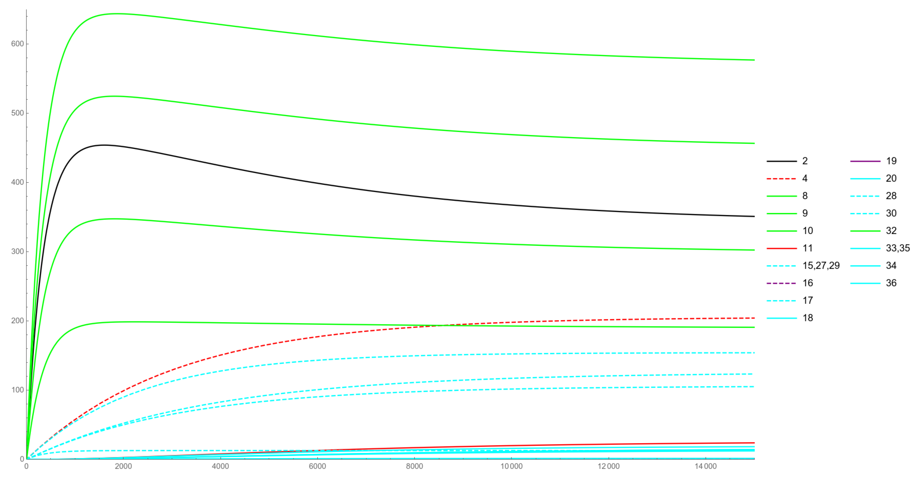
We observe that, for $\mathrm{k}=2,8,9,10,32,$ components ${\mathrm{Xi}}_{\mathrm{k}}\left(\mathrm{t}\right)$ can only be expressed via numerical integration; note that they correspond to ${\mathrm{RNA}}_{\mathrm{p}}$ and the four ceRNAs involved in the model. All the other components of $\mathrm{Xi}\left(\mathrm{t}\right)$ are either constant functions or can be expressed in closed form, in terms of the exponential function; among the latter, it is ${\mathrm{Xi}}_{15}\left(\mathrm{t}\right)={\mathrm{Xi}}_{27}\left(\mathrm{t}\right)={\mathrm{Xi}}_{29}\left(\mathrm{t}\right)$ and ${\mathrm{Xi}}_{33}\left(\mathrm{t}\right)={\mathrm{Xi}}_{35}\left(\mathrm{t}\right).$ The IVP solution to the Physiological case is plotted in Figure 3.

At this point, a modified IVP is built, formed by (12) with the coefficients ${\mathrm{c}}_{\mathrm{j}}$ in Table 4, and with initial conditions provided by the values of the Physiological solution components $\mathrm{Xi}\left(\mathrm{t}\right)$ evaluated at time ${\mathrm{T}}_1.$ One exception to the newly computed initial conditions is ${\mathrm{Xi}}_{13}\left(\mathrm{t}\right),$ whose originally null value is modified so that ${\mathrm{Xi}}_{13}\left({\mathrm{T}}_1\right)=2;$ this corresponds to considering an IVP which we denominate Ectopic Expression problem and whose solution is illustrated in Figure 4.

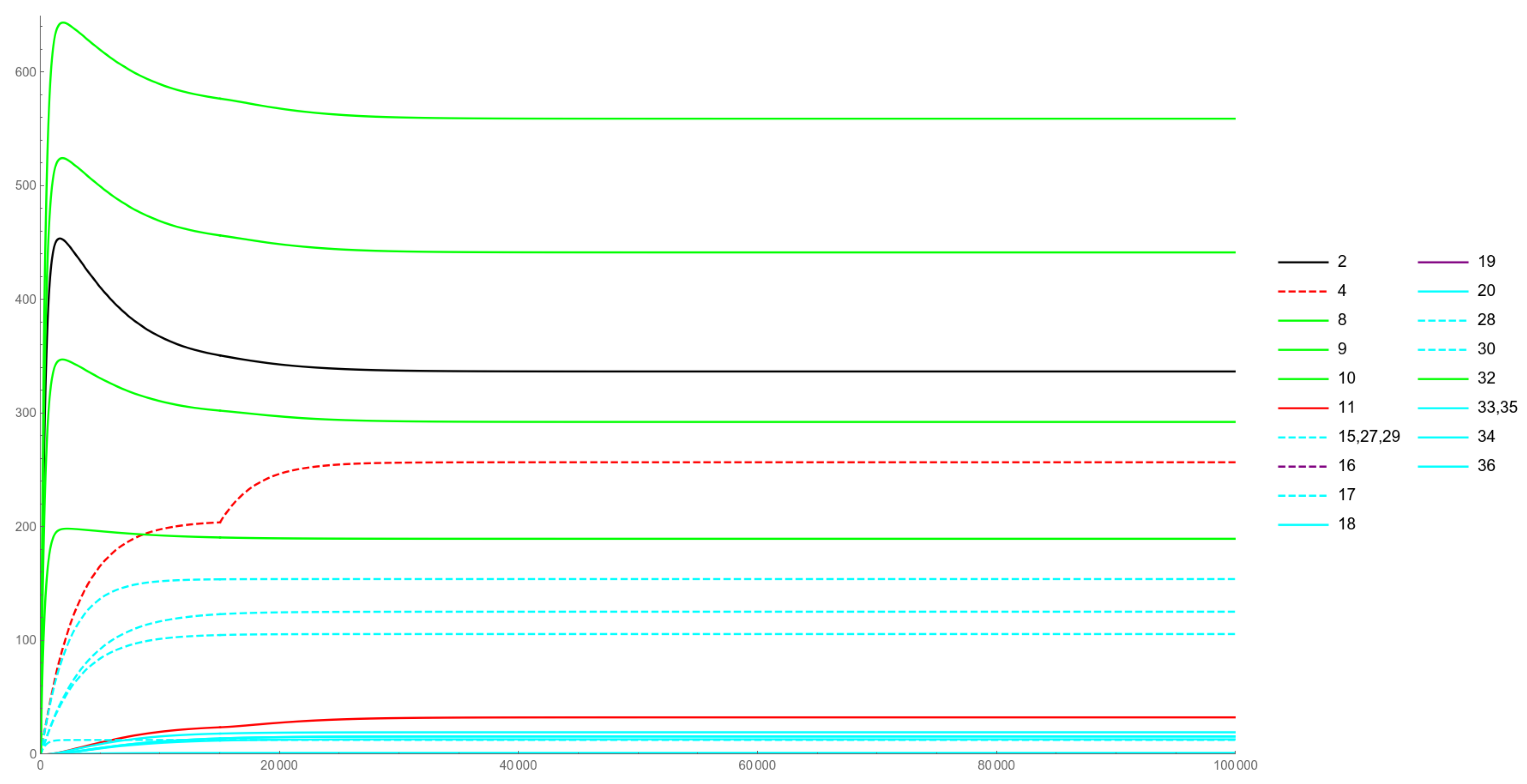
A different experiment is also considered, formed by (12) with the coefficients ${\mathrm{c}}_{\mathrm{j}}$ of Table 4, and with an exception inserted in the new initial conditions (namely, the values of the Physiological solution evaluated at ${\mathrm{T}}_1$): the value of ${\mathrm{Xi}}_3\left(\mathrm{t}\right),$ originally equal to $2,$ is modified to become ${\mathrm{Xi}}_3\left({\mathrm{T}}_1\right)=5;$ this corresponds to forming another IVP, denominated Duplication problem, whose solution is given in Figure 5.

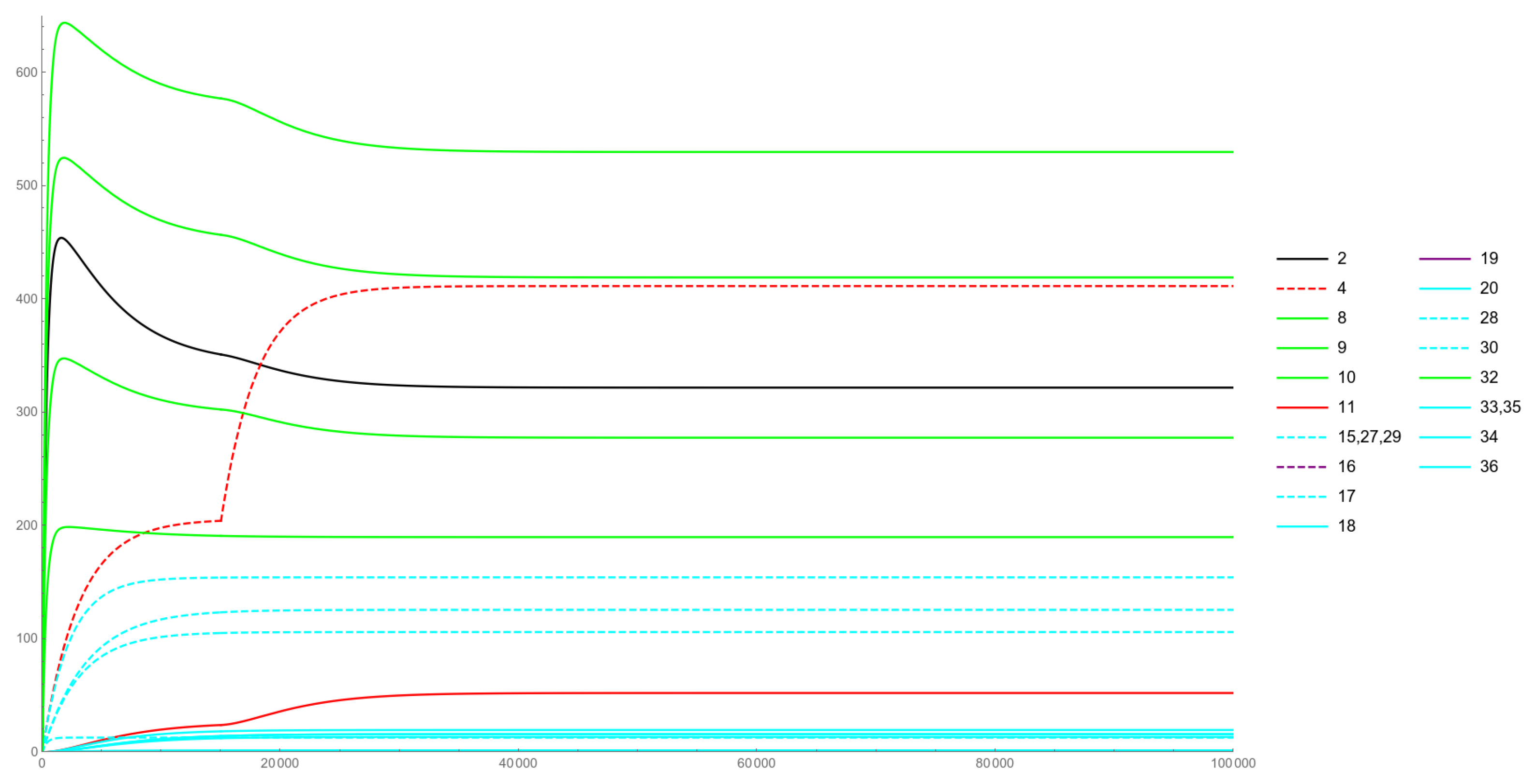
A further experiment is finally carried out; this time, an exception is inserted in the coefficients ${\mathrm{c}}_{\mathrm{j}}$ of Table 4, by setting ${\mathrm{c}}_3=3.4\times {10}^{-2}.$ The new IVP (12), whose new initial conditions are the values of the Physiological solution evaluated at ${\mathrm{T}}_1,$ is named Increased Expression problem; its solution is given in Figure 6.

By integrating each of the three modified IVPs over the time interval $[{\mathrm{T}}_1,\mathrm{T}],$ where ${\mathrm{T}}_1=1.5\times {10}^4$ and $\mathrm{T}={10}^5,$ the corresponding final solution $\mathrm{X}\left(\mathrm{t}\right)$ is obtained, whose components can be outlined as follows, in all the cases considered:

$$\begin{array}{cc}{\mathrm{X}}_{\mathrm{k}}\left(\mathrm{t}\right)\mathrm{has\; only\; numerical\; form}\hfill & \mathrm{k}=2,8,9,10,32,\hfill \\ {\mathrm{X}}_{\mathrm{k}}\left(\mathrm{t}\right)\mathrm{has\; closed\; form}\hfill & \mathrm{k}=4,11,15,\mathbf{16},17,18,\mathbf{19},20,28,30,33,34,36,\hfill \\ \phantom{{\mathrm{X}}_{\mathrm{k}}\left(\mathrm{t}\right)}\mathrm{with}\hfill & {\mathrm{X}}_{15}\left(\mathrm{t}\right)={\mathrm{X}}_{27}\left(\mathrm{t}\right)={\mathrm{X}}_{29}\left(\mathrm{t}\right),{\mathrm{X}}_{33}\left(\mathrm{t}\right)={\mathrm{X}}_{35}\left(\mathrm{t}\right),\hfill \\ {\mathrm{X}}_{\mathrm{k}}\left(\mathrm{t}\right)=2\hfill & \mathrm{k}=1,5,6,7,12,\mathbf{13},14,21,23,24,26,\hfill \\ {\mathrm{X}}_{\mathrm{k}}\left(\mathrm{t}\right)=0\hfill & \mathrm{k}=25,31,37,\hfill \\ {\mathrm{X}}_{\mathrm{k}}\left(\mathrm{t}\right)=4\hfill & \mathrm{k}=3,22.\hfill \end{array}$$

(14)

Observations that are similar to those related to the intermediate Physiological solution $\mathrm{Xi}\left(\mathrm{t}\right)$ can also be made on the solution $\mathrm{X}\left(\mathrm{t}\right)$ obtained at the end of the second integration step. As before, ${\mathrm{X}}_2\left(\mathrm{t}\right),{\mathrm{X}}_8\left(\mathrm{t}\right),{\mathrm{X}}_9\left(\mathrm{t}\right),{\mathrm{X}}_{10}\left(\mathrm{t}\right),{\mathrm{X}}_{32}\left(\mathrm{t}\right)$ cannot be expressed in closed form and require numerical integration, while the remaining components of $\mathrm{X}\left(\mathrm{t}\right)$ are constant or possess an explicit exponential expression; in particular, equalities are verified by the following closed-form components of the solution: ${\mathrm{X}}_{15}\left(\mathrm{t}\right)={\mathrm{X}}_{27}\left(\mathrm{t}\right)={\mathrm{X}}_{29}\left(\mathrm{t}\right)$ and ${\mathrm{X}}_{33}\left(\mathrm{t}\right)={\mathrm{X}}_{35}\left(\mathrm{t}\right).$

5. Discussion

Figure 3, Figure 4, Figure 5 and Figure 6 illustrate the non-constant solution components to the various IVPs considered in Section 4.

The color coding employed is as follows. The green curves represent the levels of the various ceRNAs, while the black curve represents ${\mathrm{RNA}}_{\mathrm{p}}.$ Cyan curves are the considered miRNAs (dashed style) and their lmiRNA counterparts (solid style). Those miRNAs that are subject to change are rendered in red or purple (dashed curves), while their loaded versions are given as solid-style curves in the same red or purple colors.

Figure 3 refers to a Physiological case. Here, the initial conditions reflect the various species that are normally present in the human brain under physiological conditions. After an initial steep increase in the levels of RNAp and ceRNAs, a slight decrease can be observed, due to the action of the lmiRNAs on their targets, after both expression of their miRNA and loading into RISC have occurred. From a biological perspective, our model mirrors what should happen inside a brain cell under physiological conditions: since PTEN is an onco-suppressor gene, it is important that its levels reach an equilibrium and do not drop dramatically, even when miRNAs are present that are capable to down-regulate it.

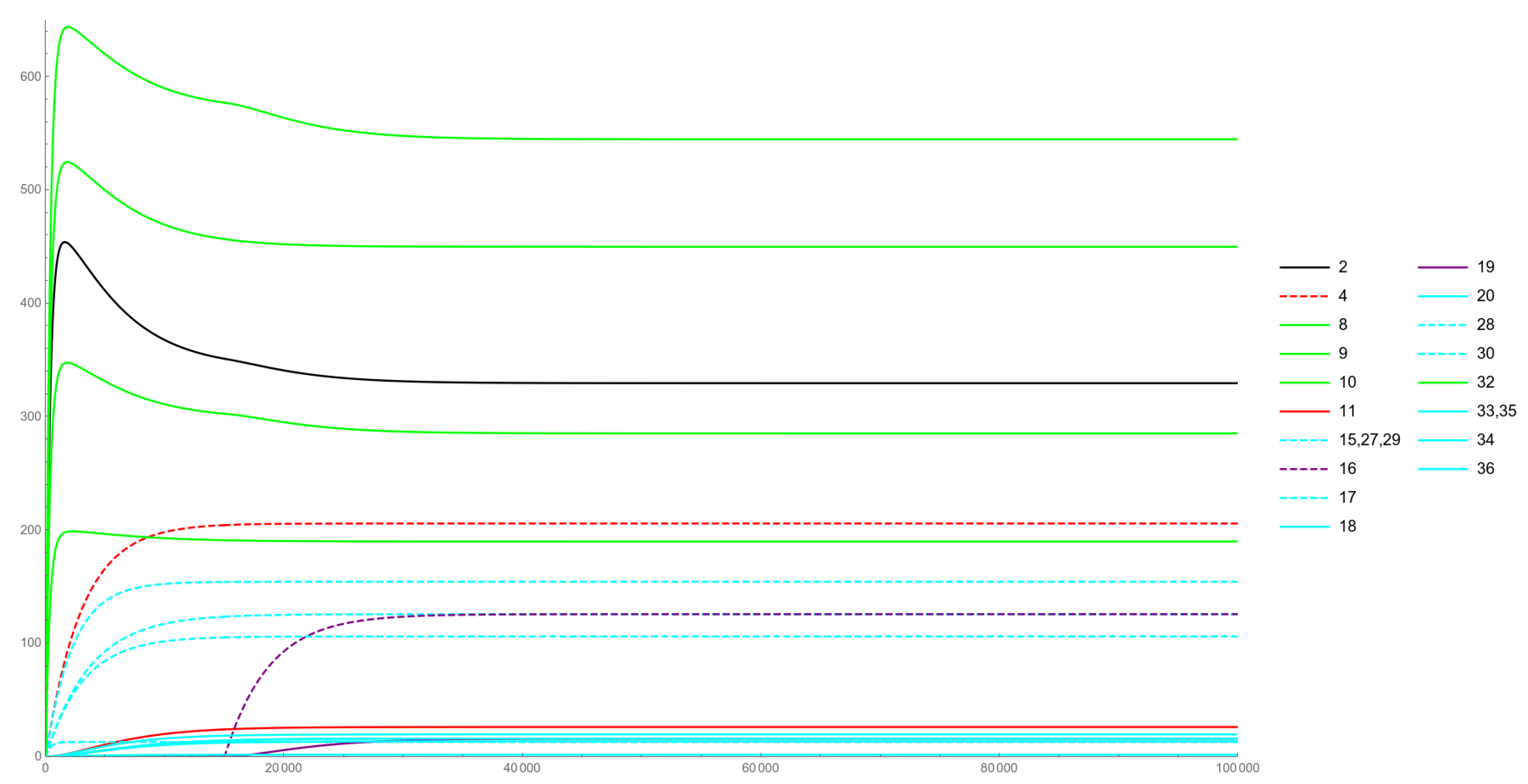
Figure 4 is related to an Ectopic Expression case. The sudden expression of a miRNA and its loaded counterpart are simulated here, assumed to occur at the instant of time ${\mathrm{T}}_1$ and respectively rendered as dashed-purple and solid-purple curves. The ectopic expression of a gene (i.e., the presence of its product in a biological context in which it should not be present) has been observed in many pathological conditions, including tumors. As Figure 4 describes, our model predicts an (obvious) increase in the mRNA levels of the newly appeared miRNA, together with a small overall decrease in the levels of ${\mathrm{RNA}}_{\mathrm{p}}$ and ceRNAs. This may be explained by the levels of the newly inserted lmiRNA, which turn out to be comparable to the other lmiRNAs: in other words, even if the new miRNA gets expressed, only a small fraction of it can be loaded into RISC and can, thus, become capable of affecting ${\mathrm{RNA}}_{\mathrm{p}}$ levels.

Figure 5 illustrates a Duplication case, related to the simulation of the effect of the duplication of a gene: this translates into the presence of an additional copy of the gene being expressed inside the cell, together with an overall increase in the levels of its products. As shown in Figure 5, at the time ${\mathrm{T}}_1$ of duplication, a noticeable leap in the miRNA product can be observed (dashed red curve), as well as a small upsurge in the lmiRNA levels (solid red curve). The overall effect on RNAp (and the targeted ceRNAs) levels remains modest, as in the previous case of ectopic expression of a gene.

Figure 6 refers to an Increased Expression case, that is the simulation of the increased expression of an already present gene, a condition usually referred to as over-expression in biology and that can lead to pathological conditions, similar to those potentially caused by duplications or ectopic expressions. Starting from ${\mathrm{T}}_1,$ a sharp increase can be observed in the miRNA levels, as well as in the related lmiRNA species (dashed-red and solid-red curves in Figure 6). Unlike in cases of ectopic expression and duplication, here the miRNA curve soon overtakes the RNAp curve. However, the overall levels of RNAp are not subject to a more significant decrease than in the previous two simulation cases. This again seems to imply the robustness of the ceRNAs network in acting as off-targets and the loading into RISC as a critical step in regulating the levels of the targeted species.

6. Conclusions

Focus of this work is the modeling of a gene regulatory network, in particular that of the miRNAs of PTEN, and its impact on target species, the latter being mRNAs or ceRNAs. To this aim, a model is designed, related to sixty-seven chemical reactions in which thirty-seven species appear, that describes the regulation of the PTEN gene and involves, in particular, four ceRNAs and nine miRNAs. To deal with the large dimensions involved, the simulations presented relate to a simplified deterministic model, in which the intrinsic stochasticity of biochemical reactions is neglected, and show the behavior of the species considered in some biologically relevant situations, as explained in Section 5.

From a biological perspective, our model, although simplified, is able to mirror parts of the biological subtext that lies behind various alterations and can lead to many pathologies, such as GBM, in our specific case. In addition, our results suggest a role for RISC, not just as a restrictive step, but as a kind of safety mechanism. Loading into RISC, being a biological bottleneck, ensures that alterations (or even fluctuations) in miRNA levels will not be capable to directly (and dramatically) affect the entire network, thereby increasing its robustness.

In the model presented, initial conditions and reaction rates are not experimentally determined, but rather inferred from the literature available on the topic; despite this, the model is capable to behave properly, that is, in a biologically reasonable fashion. The interest remains related to the possibility of testing our model on empirical data, currently not available, due to the complexity of processes involved in obtaining them, making this task an auspicable and advisable future work.

References

- Lee, Y.R.; Chen, M.; Pandolfi, P.P. The functions and regulation of the PTEN tumour suppressor: New modes and prospects. Nat. Rev. Mol. Cell Biol. 2018, 19, 547–562. [Google Scholar] [CrossRef]
- Carracedo, A.; Alimonti, A.; Pandolfi, P.P. PTEN level in tumor suppression: How much is too little? Cancer Res. 2011, 71, 629–633. [Google Scholar] [CrossRef] [Green Version]
- Carletti, M.; Montani, M.; Meschini, V.; Bianchi, M.; Radici, L. Stochastic modelling of PTEN regulation in brain tumors: A model for glioblastoma multiforme. Math. Biosci. Eng. 2015, 12, 965–981. [Google Scholar]
- Karreth, F.A.; Tay, Y.; Perna, D.; Ala, U.; Tan, S.M.; Rust, A.G.; DeNicola, G.; Webster, K.A.; Weiss, D.; Perez–Mancera, P.A.; et al. In vivo identification of tumor–suppressive PTEN ceRNAs in an oncogenic BRAF–induced mouse model of melanoma. Cell 2011, 147, 382–395. [Google Scholar] [CrossRef] [PubMed] [Green Version]
- Sumazin, P.; Yang, X.; Chiu, H.-S.; Chung, W.-J.; Iyer, A.; Llobet-Navas, D.; Rajbhandari, P.; Bansal, M.; Guarnieri, P.; Silva, J.; et al. An extensive microRNA–mediated network of RNA–RNA interactions regulates established oncogenic pathways in glioblastoma. Cell 2011, 147, 370–381. [Google Scholar] [CrossRef] [Green Version]
- Orlic-Milacic, M.; Salmena, L.; Carracedo, A. PTEN Regulation [id: R–HSA–6807070.2, Species: Homo Sapiens], Reactome, Release 17. 2017. Available online: https://reactome.org/PathwayBrowser/#/R-HSA-6807070 (accessed on 23 July 2021).
- Jassal, B.; Matthews, L.; Viteri, G.; Gong, C.; Lorente, P.; Fabregat, A.; Sidiropoulos, K.; Cook, J.; Gillespie, M.; Haw, R.; et al. The reactome pathway knowledgebase. Nucleic Acids Res. 2020, 48, D498–D503. [Google Scholar] [CrossRef] [PubMed]
- Stelzer, G.; Rosen, N.; Plaschkes, I.; Zimmerman, S.; Twik, M.; Fishilevich, S.; Stein, T.I.; Nudel, R.; Lieder, I.; Mazor, Y.; et al. The GeneCards Suite: From gene data mining to disease genome sequence analyses. Curr. Protoc. Bioinform. 2016, 54, 1.30.1–1.30.33. [Google Scholar] [CrossRef] [PubMed]
- Papatheodorou, I.; Moreno, P.; Manning, J.; Muñoz-Pomer Fuentes, A.; George, N.; Fexova, S.; Fonseca, N.A.; Füllgrabe, A.; Green, M.; Huang, N.; et al. Expression Atlas update: From tissues to single cells. Nucleic Acids Res. 2020, 48, D77–D83. [Google Scholar] [CrossRef] [PubMed] [Green Version]
- Poliseno, L.; Pandolfi, P.P. PTEN ceRNA networks in human cancer. Methods 2015, 77–78, 41–50. [Google Scholar] [CrossRef] [PubMed]
- Reichholf, B.; Herzog, V.A.; Fasching, N.; Manzenreither, R.A.; Sowemimo, I.; Ameres, S.L. Time-resolved small RNA sequencing unravels the molecular principles of microRNA homeostasis. Mol. Cell 2019, 75, 756–768. [Google Scholar] [CrossRef] [PubMed]
- Hausser, J.; Syed, A.P.; Selevsek, N.; van Nimwegen, E.; Jaskiewicz, L.; Aebersold, R.; Zavolan, M. Timescales and bottlenecks in miRNA–dependent gene regulation. Mol. Syst. Biol. 2013, 9, 711. [Google Scholar] [CrossRef]
- De, N.; Young, L.; Lau, P.-W.; Meisner, N.-C.; Morrissey, D.V.; MacRae, I.J. Highly complementary target RNAs promote release of guide RNAs from human Argonaute2. Mol. Cell 2013, 50, 344–355. [Google Scholar] [CrossRef] [Green Version]
- Burrage, K.; Tian, T.; Burrage, P. A multi–scaled approach for simulating chemical reaction systems. Prog. Biophys. Mol. Biol. 2004, 85, 217–234. [Google Scholar] [CrossRef]
- Cao, Y.; Li, H.; Petzold, L. Efficient formulation of the stochastic simulation algorithm for chemically reacting systems. J. Chem. Phys. 2004, 121, 4059–4067. [Google Scholar] [CrossRef]
- Gillespie, D.T. Exact stochastic simulation of coupled chemical reactions. J. Chem. Phys. 1977, 81, 2340–2361. [Google Scholar] [CrossRef]
- Guo, Y.; Liu, J.; Elfenbein, S.J.; Ma, Y.; Zhong, M.; Qiu, C.; Ding, Y.; Lu, J. Characterization of the mammalian miRNA turnover landscape. Nucleic Acids Res. 2015, 43, 2326–2341. [Google Scholar] [CrossRef] [PubMed]
- Marzi, M.J.; Ghini, F.; Cerruti, B.; de Pretis, S.; Bonetti, P.; Giacomelli, C.; Gorski, M.M.; Kress, T.; Pelizzola, M.; Muller, H.; et al. Degradation dynamics of microRNAs revealed by a novel pulse–chase approach. Genome Res. 2016, 26, 554–565. [Google Scholar] [CrossRef] [Green Version]
- Price, D.H. Transient pausing by RNA polymerase II. Proc. Natl. Acad. Sci. USA 2018, 115, 4810–4812. [Google Scholar] [CrossRef] [Green Version]
- Sheu-Gruttadauria, J.; MacRae, I.J. Structural Foundations of RNA Silencing by Argonaute. J. Mol. Biol. 2017, 429, 2619–2639. [Google Scholar] [CrossRef] [PubMed]
- Singh, J.; Padgett, R.A. Rates of in situ transcription and splicing in large human genes. Nat. Struct. Mol. Biol. 2009, 16, 1128–1133. [Google Scholar] [CrossRef] [PubMed] [Green Version]
- Van den Berg, A.; Mols, J.; Han, J. RISC-target interaction: Cleavage and translational suppression. Biochim. Biophys. Acta 2008, 1779, 668–677. [Google Scholar] [CrossRef] [PubMed] [Green Version]
- Hindmarsh, A.C.; Petzold, L.R. Livermore Solver for Ordinary Differential Equations (LSODA) for Stiff or Non–Stiff System. Nuclear Energy Agency (NEA) of the Organisation for Economic Co–operation and Development (OECD). 2005. Available online: http://inis.iaea.org/search/search.aspx?orig$_{}$q=RN:41086668 (accessed on 23 July 2021).
- Sofroniou, M.; Knapp, R. Advanced Numerical Differential Equation Solving in Mathematica; WRI Tutorial; Wolfram Research Inc.: Champaign, IL, USA, 2003. [Google Scholar]
- Bashforth, F.; Adams, J.C. An Attempt to Test the Theories of Capillary Action by Comparing the Theoretical and Measured Forms of Drops of Fluid; Cambridge University Press: Cambridge, UK, 1883. [Google Scholar]
- Shampine, L.F. Variable order Adams codes. Comput. Math. Appl. 2002, 44, 749–761. [Google Scholar] [CrossRef] [Green Version]
- Curtiss, C.F.; Hirschfelder, J.O. Integration of stiff equations. Proc. Natl. Acad. Sci. USA 1952, 38, 35–243. [Google Scholar] [CrossRef] [PubMed] [Green Version]
- Petzold, L.R. Automatic Selection of Methods for Solving Stiff and Nonstiff Systems of Ordinary Differential Equations. SIAM J. Sci. Stat. Comput. 1983, 4, 136–148. [Google Scholar] [CrossRef]
- Sofroniou, M.; Spaletta, G. Stiffness Detection Revisited; Series in Applied Sciences; Universitas Studiorum: Mantua, Italy, 2019; Volume 2, pp. 179–203. [Google Scholar]
- Lambert, J.D. Numerical Methods for Ordinary Differential Systems: The Initial Value Problem; John Wiley & Sons: Chichester, UK, 1991. [Google Scholar]
Figure 1.
Proposed model of the miRNA regulatory network for PTEN.
Figure 2.
Stoichiometric matrix for the chemical reactions (1b).
Figure 3.
Physiological case.
Figure 4.
Ectopic Expression case.
Figure 5.
Duplication case.
Figure 6.
Increased Expression case.