Analysis of External Debt Sustainability in Mongolia: an Estimated DSGE Approach

Abstract

In this study, we assess the effects of the structural shocks on the external debt sustainability in Mongolia, based on an estimated small open economy (SOE) dynamic stochastic general equilibrium (DSGE) model with the traded, the non-traded, and the mining sectors. The impulse response results show that the traded sector’s productivity shock, the commodity price shock, the mining output shock, and the foreign interest-rate shock have a decreasing effect on external debt accumulation in Mongolia, whereas the non-traded sector’s productivity shock, the household preference shock, and the government spending shock have an increasing effect on the same. Furthermore, we assess Mongolia’s external debt sustainability under the COVID−19 pandemic shock. Under our assumed pandemic scenario, Mongolia’s external debt will increase by 30% from its steady state over the next 10–28 quarters. Our recommended solution in this study is to develop the traded sector, instead of the mining sector, to maintain sustainability of the external debt and to decrease vulnerability of the economy.

1. Introduction

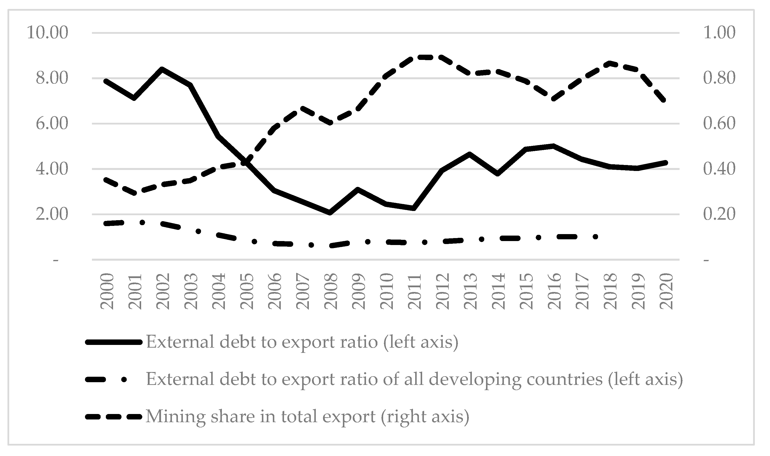
While Mongolia’s mining sector has been experiencing a boom, its external debt has also been increasing substantially over the last decade. In other words, the defining feature of the current state of the Mongolian economy is the recent boom in the mining sector as well as in external indebtedness (Figure 1). Determining the factors responsible for the high growth rate of the country’s external debt is critical for external debt management, because high external debt has a decelerating effect on a country’s economic development, as reported by recent debt–growth nexus literature [1,2,3,4].

The purpose of this study is to assess the factors influencing external debt sustainability in Mongolia by constructing and estimating a small open economy (SOE) dynamic stochastic general equilibrium (DSGE) model that incorporates the most important features of the Mongolian economy. To the best of our knowledge, the study of Li et al. [5] is the only one that has analyzed the external debt sustainability of Mongolia using the DSGE model. The author constructed a medium-scale DSGE model, which has three sectors (traded, non-traded, and resource) and includes several real frictions, such as capital adjustment costs, non-Ricardian households, public investment inefficiency, and absorptive capacity constraints. The model structure applied in Li et al. [5] is similar to that of average low-income countries (LICs) [6], Central African Economic and Monetary Community (CEMAC) and Angola [7], and for average LICs [8]. These DSGE models incorporate features of resource-rich LICs, such as sovereign wealth funds and government capital. With calibrated initial values and parameters based on national accounting data, the authors run model simulations to assess alternative fiscal policy rules under several different scenarios, such as commodity price drop and delay of mining constructions, to assess the sustainability of external debt. However, these DSGE models are absent from important structural shocks, shocks’ identification, and parameter estimation.

In addition to Li et al. [5], there are several other DSGE studies on the Mongolian economy. New Keynesian DSGE (NK-DSGE) models aim to evaluate the effectiveness of monetary policy on macroeconomic variables and determine the monetary policy rules. In this vein, it is found that the contemporaneous inflation responsive rule fulfills the Taylor principle in the recent phase of an inflation targeting period, and the response is weaker than other emerging Asian inflation targeting countries [9]. The NK-DSGE model structure employed by Taguchi and Gunbileg [9] was similar to the one in Gali and Monacelli [10]. Moreover, the importance of the exchange rate pass-through effect in the Mongolian economy was assessed by calibrating parameters for Gali and Monacelli [10] and running model simulations under four different degrees of pass-through effect [11]. In addition to these two SOE NK-DSGE studies with a similar architecture but with different objectives, Doojav and Batmunkh [12] constructs a structural model with NK-DSGE features to assess monetary policy and macroprudential policy effects on the Mongolian economy. The authors concluded that the policy rate has a stronger impact on inflation and exchange rates than the macroprudential policy, and a combination of these two policies reduces the welfare loss caused by the central bank’s participation in the economy. Furthermore, the SOE NK-DSGE model is applied to identify the natural rate of interest in Mongolia by estimating the model using the Bayesian method and filtering the unobserved components of the natural rate of interest, inflation target, equilibrium output growth, and equilibrium exchange rate using the Kalman smoother [13]. To the best of our knowledge, no other study has applied an estimated DSGE model to assess external debt accumulation in Mongolia. By filling this gap and assessing external debt accumulation, we enrich the DSGE studies on the Mongolian economy, in addition to assessing the structural shocks’ impact on external debt accumulation in Mongolia.

Our main contribution to the DSGE literature on the Mongolian economy is to construct an estimable SOE-DSGE model (DSGE models applied in Li et al. [5], Melina et al. [8] and Berg et al. [6,7] are non-estimable, as the authors assume several contingent rules that make a linear approximation of the policy function impossible), augmenting the standard non-traded sector’s DSGE model in textbooks [14,15] with the mining sector [5,8] and the preference shock [16]. The DSGE model applied in Li et al. [5] is non-estimable while the standard non-traded sector DSGE model is absent from the mining sector and the preference shock. Therefore, we build an estimable DSGE model reflecting current features of the Mongolian economy, identify the structural shocks using the Bayesian estimation method and assess the structural shocks’ effect on the external debt sustainability of Mongolia. Finally, we assess Mongolia’s external debt sustainability under the COVID−19 pandemic shock by incorporating multiple structural shocks into our estimated DSGE model.

2. The Model

The general philosophy of the mining sector’s inclusion in the DSGE model is similar to that of Li et al. [5], Melina et al. [8] and Berg et al. [6,7], but the investment decision making process shifts from firms to households along with Uribe and Schmitt-Grohe [14]. We modified the DSGE model by incorporating recent achievements in the emerging market real business cycle (RBC) literature, such as a preference shock [16], to improve the structural shocks’ identification procedure. Finally, we employ portfolio adjustment cost [17] for closing the economy and incorporating financial friction into the DSGE model.

2.1. The Household’s Intertemporal Optimization

Households maximize their lifetime utility function subject to their budget constraints. Following the open economy DSGE literature [16,17,18], the household’s preference function is non-separable with respect to consumption and labor, as follows:

$$\underset{{\mathrm{c}}_{\mathrm{t}}{, \mathrm{i}}_{\mathrm{t}}{, \mathrm{h}}_{\mathrm{t}}{, \mathrm{k}}_{\mathrm{t}}{, \mathrm{b}}_{\mathrm{t}}}{\max }{\mathrm{E}}_0{{\displaystyle \sum }}_{\mathrm{t}=0}^{\infty }{\mathsf{\nu }}_{\mathrm{t}}{\mathsf{\beta }}^{\mathrm{t}}\frac{{\left({\mathrm{c}}_{\mathrm{t}}-{ \mathsf{\theta }}_{\mathrm{L}}{\mathsf{\omega }}^{-1}{\mathrm{h}}_{\mathrm{t}}^{\mathsf{\omega }}\right)}^{1-\mathsf{\sigma }}}{1 - \mathsf{\sigma }},$$

(1)

where ${\mathrm{v}}_{\mathrm{t}}$ is the preference shock, which follows the AR (1) process (Equation (2)),

$$\ln \left({\mathrm{v}}_{\mathrm{t}}\right)=\left(1 -{ \mathsf{\rho }}_{\mathrm{v}}\right)\ln \left(\mathrm{v}\right){+\mathsf{\rho }}_{\mathrm{v}}\ln \left({\mathrm{v}}_{\mathrm{t}-1}\right){+\mathsf{\epsilon }}_{\mathrm{t}}^{\mathrm{v}}{; \mathsf{\epsilon }}_{\mathrm{t}}^{\mathrm{v}}\sim \mathrm{NID}\left({0,\mathsf{\sigma }}_{\mathrm{v}}^2\right),$$

(2)

${\mathsf{\beta }}^{\mathrm{t}}$ is the discount factor, ${\mathrm{c}}_{\mathrm{t}}$ is the basket of consumption at time $\mathrm{t}$,${ \mathrm{w}}_{\mathrm{t}}$ is the wage rate, and ${\mathrm{h}}_{\mathrm{t}}$ is hours worked. Households’ period budget constraint and motion of capital are specified as follows:

$${\mathrm{p}}_{\mathrm{t}}{\mathrm{c}}_{\mathrm{t}}{+\mathrm{p}}_{\mathrm{t}}{\mathrm{i}}_{\mathrm{t}}{+\mathrm{b}}_{\mathrm{t}}{=\mathrm{r}}_{\mathrm{t}}^{\mathrm{k}}{\mathrm{p}}_{\mathrm{t}}{\mathrm{k}}_{\mathrm{t}-1}{+\mathrm{r}}_{\mathrm{t}-1}^{*}{\mathrm{b}}_{\mathrm{t}-1}{+\mathrm{p}}_{\mathrm{t}}{\mathrm{w}}_{\mathrm{t}}{\mathrm{h}}_{\mathrm{t}}-{ \mathrm{p}}_{\mathrm{t}}{\mathrm{t}}_{\mathrm{t}}{+\mathrm{p}}_{\mathrm{t}}{\mathsf{\Omega }}_{\mathrm{t}} \frac{{\mathsf{\theta }}_{\mathrm{D}}}{2}{\left({\mathrm{b}}_{\mathrm{t}}- \mathrm{b}\right)}^2,$$

(3)

$${\mathrm{k}}_{\mathrm{t}}=\left(1 - \mathsf{\delta }\right){\mathrm{k}}_{\mathrm{t}-1}+\left[1 -\frac{{\mathsf{\theta }}_{\mathrm{I}}}{2}{\left(\frac{{\mathrm{i}}_{\mathrm{t}}}{{\mathrm{i}}_{\mathrm{t}-1}}- 1\right)}^2\right]{\mathrm{i}}_{\mathrm{t}},$$

(4)

where ${\mathrm{p}}_{\mathrm{t}}$ is general price—unit consumption basket in terms of the tradable good’s price, ${\mathrm{i}}_{\mathrm{t}}$ is the investment at time $\mathrm{t}$, ${\mathrm{b}}_{\mathrm{t}}$ is a one-period foreign bond (asset) dominated in the tradable good’s price, whose gross interest rate is ${\mathrm{r}}_{\mathrm{t}}^{*}$, which follows the AR(1) process (Equation (5)),

$${\mathrm{r}}_{\mathrm{t}}^{*}=\left(1 -{ \mathsf{\rho }}^{\mathrm{rf}}\right)\frac{1}{\mathsf{\beta }}{+\mathsf{\rho }}^{\mathrm{rf}}{\mathrm{r}}_{\mathrm{t}-1}^{*}{+\mathsf{\epsilon }}_{\mathrm{t}}^{\mathrm{rf}}{, \mathsf{\epsilon }}_{\mathrm{t}}^{\mathrm{rf}}\sim \mathrm{NID}\left({0,\mathsf{\sigma }}_{\mathrm{rf}}^2\right),$$

(5)

${\mathrm{r}}_{\mathrm{t}}^{\mathrm{k}}$ is the rental rate of capital, ${\mathrm{k}}_{\mathrm{t}}$ is the stock of capital at time $\mathrm{t}$, ${\mathrm{t}}_{\mathrm{t}}$ is the government’s lump-sum tax, and ${\mathsf{\Omega }}_{\mathrm{t}}$ is the total corporate profit. The term $\frac{{\mathsf{\theta }}_{\mathrm{D}}}{2}{\left({\mathrm{b}}_{\mathrm{t}}-\mathrm{b}\right)}^2$ is the convex portfolio adjustment cost; the change in foreign asset holdings relative to its steady state value requires adjustment cost. This expression is the key mechanism for closing our model to ensure a unique steady state. In the capital accumulation equation, the term $\left[1 -\frac{{\mathsf{\theta }}_{\mathrm{I}}}{2}{\left(\frac{{\mathrm{i}}_{\mathrm{t}}}{{\mathrm{i}}_{\mathrm{t} - 1}}- 1\right)}^2\right]{\mathrm{i}}_{\mathrm{t}}$ is the investment adjustment cost employed in the DSGE model [19]. With the investment adjustment cost, investment making is now a separate decision from the next period’s capital stock decision, and the investment making decision depends on Tobin’s q ratio [20]. We can write the budget constraint of the household (Equation (3)) in terms of the domestic general price level by dividing both sides by ${\mathrm{p}}_{\mathrm{t}}$ to satisfy the same price unit as the other expressions.

$${\mathrm{c}}_{\mathrm{t}}{+\mathrm{i}}_{\mathrm{t}}+\frac{{\mathrm{b}}_{\mathrm{t}}}{{\mathrm{p}}_{\mathrm{t}}}{=\mathrm{r}}_{\mathrm{t}}^{\mathrm{k}}{\mathrm{k}}_{\mathrm{t} - 1}+\frac{{\mathrm{r}}_{\mathrm{t} - 1}^{*}{\mathrm{b}}_{\mathrm{t} - 1}}{{\mathrm{p}}_{\mathrm{t}}}{+\mathrm{w}}_{\mathrm{t}}{\mathrm{h}}_{\mathrm{t}}-{ \mathrm{t}}_{\mathrm{t}}{+\mathsf{\Omega }}_{\mathrm{t}}-\frac{{\mathsf{\theta }}_{\mathrm{D}}}{{2\mathrm{p}}_{\mathrm{t}}}{\left({\mathrm{b}}_{\mathrm{t}}- \mathrm{b}\right)}^2.$$

(6)

The Lagrangian function associated with the household’s intertemporal optimization problem is as follows:

$$\mathrm{L}={\mathrm{E}}_0\left\{{{\displaystyle \sum }}_{\mathrm{t}=0}^{\mathsf{\infty }}{\mathsf{\beta }}^{\mathrm{t}}\left\{\left(\frac{{\left({\mathrm{c}}_{\mathrm{t}}-{\mathsf{\theta }}_{\mathrm{L}}{\omega }^{-1}{\mathrm{h}}_{\mathrm{t}}^{\omega }\right)}^{1-\mathsf{\sigma }}}{1-\mathsf{\sigma }}\right){\mathrm{v}}_{\mathrm{t}}-{\mathrm{q}}_{\mathrm{t}}{\mathsf{\lambda }}_{\mathrm{t}}\left({\mathrm{k}}_{\mathrm{t}}-\left(1-\mathsf{\delta }\right){\mathrm{k}}_{\mathrm{t}-1}-\left[1-\frac{{\mathsf{\theta }}_{\mathrm{I}}}{2}{\left(\frac{{\mathrm{i}}_{\mathrm{t}}}{{\mathrm{i}}_{\mathrm{t}-1}}-1\right)}^2\right]{\mathrm{i}}_{\mathrm{t}}\right)-{\mathsf{\lambda }}_{\mathrm{t}}\left({\mathrm{c}}_{\mathrm{t}}+{\mathrm{i}}_{\mathrm{t}}+\frac{{\mathrm{b}}_{\mathrm{t}}}{{\mathrm{p}}_{\mathrm{t}}}-{\mathrm{r}}_{\mathrm{t}}^{\mathrm{k}}{\mathrm{k}}_{\mathrm{t}-1}-\frac{{\mathrm{r}}_{\mathrm{t}-1}^{*}{\mathrm{b}}_{\mathrm{t}-1}}{{\mathrm{p}}_{\mathrm{t}}}-{\mathrm{w}}_{\mathrm{t}}{\mathrm{h}}_{\mathrm{t}}+{\mathrm{t}}_{\mathrm{t}}-{\mathsf{\Omega }}_{\mathrm{t}}+\frac{{\mathsf{\theta }}_{\mathrm{D}}}{{2\mathrm{p}}_{\mathrm{t}}}{\left({\mathrm{b}}_{\mathrm{t}}-\mathrm{b}\right)}^2\right)\right\}\right\},$$

(7)

where ${\mathsf{\lambda }}_{\mathrm{t}}$ is the Lagrangian multiplier for the household’s budget constraint, and ${\mathrm{q}}_{\mathrm{t}}$ is Tobin’s marginal $\mathrm{q}$ ratio. By taking the first derivatives from the Lagrangian function with respect to consumption ${\mathrm{c}}_{\mathrm{t}}$, external debt ${\mathrm{b}}_{\mathrm{t}}$, capital ${\mathrm{k}}_{\mathrm{t}}$ and investment ${\mathrm{i}}_{\mathrm{t}}$, we can write the following first order conditions (FOCs).

The FOC with respect to consumption:

$${\mathsf{\lambda }}_{\mathrm{t} }={\left({\mathrm{c}}_{\mathrm{t}}-\frac{{\mathsf{\theta }}_{\mathrm{L}}{\mathrm{h}}^{\mathsf{\omega }}}{\mathsf{\omega }}\right)}^{- \mathsf{\sigma }}{\mathrm{v}}_{\mathrm{t}}.$$

(8)

The FOC with respect to foreign bond:

$${\mathsf{\lambda }}_{\mathrm{t}}\left({1+\mathsf{\theta }}_{\mathrm{D}}\left({\mathrm{b}}_{\mathrm{t} }- \mathrm{b}\right)\right)=\mathsf{\beta }\left(\frac{{\mathsf{\lambda }}_{\mathrm{t}+1}{\mathrm{r}}_{\mathrm{t}}^{*}{\mathrm{p}}_{\mathrm{t}}}{{\mathrm{p}}_{\mathrm{t}+1}}\right).$$

(9)

The FOC with respect to capital:

$${\mathsf{\lambda }}_{\mathrm{t}}{\mathrm{q}}_{\mathrm{t}}{=\mathsf{\beta }\mathsf{\lambda }}_{\mathrm{t}+1}\left({\mathrm{r}}_{\mathrm{t}+1}^{\mathrm{k}}+\left(1 - \mathsf{\delta }\right){\mathrm{q}}_{\mathrm{t}+1}\right).$$

(10)

The FOC with respect to labor:

$${\mathsf{\theta }}_{\mathrm{L}}{\mathrm{h}}_{\mathrm{t}}^{\mathsf{\omega } - 1}{=\mathrm{w}}_{\mathrm{t}}.$$

(11)

The FOC with respect to investment:

$${1=\mathrm{q}}_{\mathrm{t}}\left[1 -\frac{{\mathsf{\theta }}_{\mathrm{I}}}{2}{\left(\frac{{\mathrm{i}}_{\mathrm{t}}}{{\mathrm{i}}_{\mathrm{t} - 1}}- 1\right)}^2-{ \mathsf{\theta }}_{\mathrm{I}}\left(\frac{{\mathrm{i}}_{\mathrm{t}}}{{\mathrm{i}}_{\mathrm{t} - 1}}\right)\left(\frac{{\mathrm{i}}_{\mathrm{t}}}{{\mathrm{i}}_{\mathrm{t} - 1}}- 1\right)\right]{+\mathsf{\theta }}_{\mathrm{I}}\mathsf{\beta }\frac{{ \mathsf{\lambda }}_{\mathrm{t}+1}}{{\mathsf{\lambda }}_{\mathrm{t}}}{\mathrm{q}}_{\mathrm{t}+1}\left[{\left(\frac{{\mathrm{i}}_{\mathrm{t}+1}}{{\mathrm{i}}_{\mathrm{t}}}\right)}^2\left(\frac{{\mathrm{i}}_{\mathrm{t}+1}}{{\mathrm{i}}_{\mathrm{t}}}- 1\right)\right].$$

(12)

2.2. The Household′s Intra-Temporal Decision

The household’s consumption basket consists of tradable good ${\mathrm{c}}_{\mathrm{t}}^{\mathrm{T}}$ and non-tradable good ${\mathrm{c}}_{\mathrm{t}}^{\mathrm{N}}$ as follows:

$${\mathrm{c}}_{\mathrm{t}}={\left[{\mathsf{\alpha }}^{\frac{1}{\mathsf{ϵ}}}{\mathrm{c}}_{\mathrm{t}}^{\mathrm{T}}{}^{\frac{\mathsf{ϵ}- 1}{\mathsf{ϵ}}}+{\left(1 - \mathsf{\alpha }\right)}^{\frac{1}{\mathsf{ϵ}}}{\mathrm{c}}_{\mathrm{t}}^{\mathrm{N}}{}^{\frac{\mathsf{ϵ}- 1}{\mathsf{ϵ}}}\right]}^{\frac{\mathsf{ϵ}}{\mathsf{ϵ}- 1}},$$

(13)

where $\mathsf{\alpha }$ indicates the share of tradable good in the consumption basket, and $\mathsf{ϵ}$ is the substitution elasticity between tradable and non-tradable goods. Households maximize the consumption basket by choosing an optimal mix of tradable and non-tradable goods subject to total expenditure as follows:

$$\underset{{\mathrm{c}}_{\mathrm{t}}^{\mathrm{T}}{,\mathrm{c}}_{\mathrm{t}}^{\mathrm{N}}}{\max }{\left[{\mathsf{\alpha }}^{\frac{1}{\mathsf{ϵ}}}{\mathrm{c}}_{\mathrm{t}}^{\mathrm{T}}{}^{\frac{\mathsf{ϵ}- 1}{\mathsf{ϵ}}}+{\left(1 - \mathsf{\alpha }\right)}^{\frac{1}{\mathsf{ϵ}}}{\mathrm{c}}_{\mathrm{t}}^{\mathrm{N}}{}^{\frac{\mathsf{ϵ}- 1}{\mathsf{ϵ}}}\right]}^{\frac{\mathsf{ϵ}}{\mathsf{ϵ}-1}}$$

(14)

Subject to:

$${\mathrm{p}}_{\mathrm{t}}^{\mathrm{T}}{\mathrm{c}}_{\mathrm{t}}^{\mathrm{T}}{+\mathrm{p}}_{\mathrm{t}}^{\mathrm{N}}{\mathrm{c}}_{\mathrm{t}}^{\mathrm{N}}{=\mathrm{A}}_{\mathrm{t}},$$

(15)

where ${\mathrm{p}}_{\mathrm{t}}^{\mathrm{T}}$ and ${\mathrm{p}}_{\mathrm{t}}^{\mathrm{N}}$ are prices of tradable and non-tradable goods, respectively, and ${\mathrm{A}}_{\mathrm{t}}$ is a given level of expenditure. As our economy is small, the tradable good’s price is taken exogenously. Therefore, we can normalize ${\mathrm{p}}^{\mathrm{T} }=1$, or the tradable good’s price is the numeraire of the model. The household’s intra-temporal optimization decision gives us the following consumption rules,

$${\mathrm{c}}_{\mathrm{t}}^{\mathrm{N}}=\left(1 - \mathsf{\alpha }\right){\left(\frac{{\mathrm{p}}_{\mathrm{t}}^{\mathrm{N}}}{{\mathrm{p}}_{\mathrm{t}}}\right)}^{-\mathsf{ϵ}}{\mathrm{c}}_{\mathrm{t}},$$

(16)

$${\mathrm{c}}_{\mathrm{t}}^{\mathrm{T}}=\mathsf{\alpha }{\left(\frac{{\mathrm{p}}_{\mathrm{t}}^{\mathrm{T}}}{{\mathrm{p}}_{\mathrm{t}}}\right)}^{-\mathsf{ϵ}}{\mathrm{c}}_{\mathrm{t}}{=\mathsf{\alpha } \mathrm{p}}_{\mathrm{t}}^{\mathsf{ϵ}}{\mathrm{c}}_{\mathrm{t}}.$$

(17)

By substituting these two consumption rules into the general consumption basket Equation (13) and considering tradable good’s price is the numeraire, we obtain the general price index rule as follows:

$${\mathrm{p}}_{\mathrm{t}}={\left[{\mathsf{\alpha }\mathrm{p}}_{\mathrm{t}}^{{\mathrm{T}}^{\mathsf{ϵ}}}+\left(1 - \mathsf{\alpha }\right){\mathrm{p}}_{\mathrm{t}}^{{\mathrm{N}}^{1-\mathsf{ϵ}}}\right]}^{\frac{1}{1-\mathsf{ϵ}}}={\left[\mathsf{\alpha }+\left(1 - \mathsf{\alpha }\right){\mathrm{p}}_{\mathrm{t}}^{{\mathrm{N}}^{1-\mathsf{ϵ}}}\right]}^{\frac{1}{1-\mathsf{ϵ}}}.$$

(18)

If we assume that the foreign country has the same general price rule as our economy, then ${\mathrm{p}}_{\mathrm{t}}$ is interpreted as a measure of the real exchange rate (the real exchange rate is rate at which one country’s consumption basket will be exchanged for another; therefore, the ratio of domestic consumption price index to foreign price, which is the numeraire of the model or equal to one, indicates the real exchange rate as long as the foreign country (rest of the world) follows the same price index rule), a higher ${\mathrm{p}}_{\mathrm{t}}$ means that our economy is experiencing real appreciation. The total investment is also divided into tradable and non-tradable goods with the same rule (Equations (16) and (17)) as consumption,

$${\mathrm{i}}_{\mathrm{t}}^{\mathrm{N}}=\left(1 - \mathsf{\alpha }\right){\left(\frac{{\mathrm{p}}_{\mathrm{t}}^{\mathrm{N}}}{{\mathrm{p}}_{\mathrm{t}}}\right)}^{-\mathsf{ϵ}}{\mathrm{i}}_{\mathrm{t}},$$

(19)

$${\mathrm{i}}_{\mathrm{t}}^{\mathrm{T}}=\mathsf{\alpha }{\left(\frac{{\mathrm{p}}_{\mathrm{t}}^{\mathrm{T}}}{{\mathrm{p}}_{\mathrm{t}}}\right)}^{-\mathsf{ϵ}}{\mathrm{i}}_{\mathrm{t}}{=\mathsf{\alpha } \mathrm{p}}_{\mathrm{t}}^{\mathsf{ϵ}}{\mathrm{i}}_{\mathrm{t}}.$$

(20)

2.3. Firms

In this DSGE model, the production sector has three types of firms: non-tradable goods producing firms, tradable goods producing firms, and mining firms. The first two firms employ the Cobb–Douglas technology [18], whereas the mining firms’ output is exogenously defined [5,8].

2.3.1. Tradable Good Producing Firm

The representative tradable good producing firm’s production technology is as follows:

$${\mathrm{y}}_{\mathrm{t}}^{\mathrm{T}}{=\mathrm{A}}_{\mathrm{t}}^{\mathrm{T}}{\mathrm{k}}_{\mathrm{t}}^{{\mathrm{T}}^{{\mathsf{\alpha }}_{\mathrm{T}}}}{\mathrm{h}}_{\mathrm{t}}^{{\mathrm{T}}^{1-{\mathsf{\alpha }}_{\mathrm{T}}}},$$

(21)

where ${\mathrm{k}}_{\mathrm{t}}^{\mathrm{T}}$ and ${\mathrm{h}}_{\mathrm{t}}^{\mathrm{T}}$ are the capital stock and labor employed in the tradable sector, respectively and ${\mathrm{A}}_{\mathrm{t}}^{\mathrm{T}}$ is the total factor productivity, which follows the AR(1) process (Equation (22)):

$$\ln \left({\mathrm{A}}_{\mathrm{t}}^{\mathrm{T}}\right)=\left(1-{\mathsf{\rho }}_{\mathrm{T}}\right)\ln \left({\mathrm{A}}^{\mathrm{T}}\right)+{\mathsf{\rho }}_{\mathrm{T}}\ln \left({\mathrm{A}}_{\mathrm{t}-1}^{\mathrm{T}}\right)+{\mathsf{\epsilon }}_{\mathrm{t}}^{\mathrm{AT}}$$

(22)

where ${\mathsf{\epsilon }}_{\mathrm{t}}^{\mathrm{AT}}\sim {\mathrm{NID}(0,\mathsf{\sigma }}_{\mathrm{AT}}^2)$ is the technology shock in the tradable sector. The tradable good producing firm’s decision is to maximize its profit subject to the given technology,

$$\underset{{\mathrm{k}}_{\mathrm{t}}^{\mathrm{T}}{,\mathrm{h}}_{\mathrm{t}}^{\mathrm{T}}}{\max (}{\mathrm{A}}_{\mathrm{t}}^{\mathrm{T}}{\mathrm{k}}_{\mathrm{t}}^{{\mathrm{T}}^{{\mathsf{\alpha }}_{\mathrm{T}}}}{\mathrm{h}}_{\mathrm{t}}^{{\mathrm{T}}^{1-{\mathsf{\alpha }}_{\mathrm{T}}}}-{ \mathrm{p}}_{\mathrm{t}}{\mathrm{w}}_{\mathrm{t}}{\mathrm{h}}_{\mathrm{t}}^{\mathrm{T}}-{ \mathrm{p}}_{\mathrm{t}}{\mathrm{r}}_{\mathrm{t}}^{\mathrm{K}}{\mathrm{k}}_{\mathrm{t}}^{\mathrm{T}}).$$

(23)

The FOC with respect to capital:

$$\begin{array}{l}{\mathsf{A}}_{\mathrm{T}}{\mathrm{A}}_{\mathrm{t}}^{\mathrm{T}}{\mathrm{k}}_{\mathrm{t}}^{{\mathrm{T}}^{{\mathsf{\alpha }}_{\mathrm{T}}-1}}{\mathrm{h}}_{\mathrm{t}}^{{\mathrm{T}}^{1-{\mathsf{\alpha }}_{\mathrm{T}}}}{=\mathrm{p}}_{\mathrm{t}}{\mathrm{r}}_{\mathrm{t}}^{\mathrm{K}} \\ {\mathsf{\alpha }}_{\mathrm{T}}{\mathrm{y}}_{\mathrm{t}}^{\mathrm{T}}={\mathrm{p}}_{\mathrm{t}}{\mathrm{r}}_{\mathrm{t}}^{\mathrm{K}}{\mathrm{k}}_{\mathrm{t}}^{\mathrm{T}}.\end{array}$$

(24)

The FOC with respect to labor:

$$(1 -{ \mathsf{\alpha }}_{\mathrm{T}}{)\mathrm{y}}_{\mathrm{t}}^{\mathrm{T}}{=\mathrm{p}}_{\mathrm{t}}{\mathrm{w}}_{\mathrm{t}}{\mathrm{h}}_{\mathrm{t}}^{\mathrm{T}}.$$

(25)

2.3.2. Non-Tradable Good Producing Firm

The representative non-tradable good producing firm’s production technology has the following form:

$${\mathrm{y}}_{\mathrm{t}}^{\mathrm{N}}{=\mathrm{A}}_{\mathrm{t}}^{\mathrm{N}}{\mathrm{k}}_{\mathrm{t}}^{{\mathrm{N}}^{{\mathsf{\alpha }}_{\mathrm{N}}}}{\mathrm{h}}_{\mathrm{t}}^{{\mathrm{N}}^{1-{\mathsf{\alpha }}_{\mathrm{N}}}},$$

(26)

where ${\mathrm{k}}_{\mathrm{t}}^{\mathrm{N}}$ and ${\mathrm{h}}_{\mathrm{t}}^{\mathrm{N}}$ are the capital stock and labor employed in the non-tradable sector, respectively, and ${\mathrm{A}}_{\mathrm{t}}^{\mathrm{N}}$ is the total factor productivity, which follows the AR(1) process (Equation (27)):

$$\ln \left({\mathrm{A}}_{\mathrm{t}}^{\mathrm{N}}\right)=\left(1 -{ \mathsf{\rho }}_{\mathrm{T}}\right)\ln \left({\mathrm{A}}^{\mathrm{N}}\right){+\mathsf{\rho }}_{\mathrm{T}}\ln \left({\mathrm{A}}_{\mathrm{t}-1}^{\mathrm{N}}\right){+\mathsf{\epsilon }}_{\mathrm{t}}^{\mathrm{AN}},$$

(27)

where ${\mathsf{\epsilon }}_{\mathrm{t}}^{\mathrm{AN}}\sim {\mathrm{NID}(0,\mathsf{\sigma }}_{\mathrm{AN}}^2)$ is the technology shock in the non-tradable sector. The non-tradable good producing firm’s decision is to maximize its profit subject to the given technology,

$$\underset{{\mathrm{k}}_{\mathrm{t}}^{\mathrm{N}}{,\mathrm{h}}_{\mathrm{t}}^{\mathrm{N}}}{\max (}{\mathrm{A}}_{\mathrm{t}}^{\mathrm{N}}{\mathrm{k}}_{\mathrm{t}}^{{\mathrm{N}}^{{\mathsf{\alpha }}_{\mathrm{N}}}}{\mathrm{h}}_{\mathrm{t}}^{{\mathrm{N}}^{1-{\mathsf{\alpha }}_{\mathrm{N}}}}-{ \mathrm{p}}_{\mathrm{t}}{\mathrm{w}}_{\mathrm{t}}{\mathrm{h}}_{\mathrm{t}}^{\mathrm{N}}-{ \mathrm{p}}_{\mathrm{t}}{\mathrm{r}}_{\mathrm{t}}^{\mathrm{K}}{\mathrm{k}}_{\mathrm{t}}^{\mathrm{N}}).$$

(28)

The FOC with respect to capital:

$${\mathsf{\alpha }}_{\mathrm{N}}{\mathrm{y}}_{\mathrm{t}}^{\mathrm{N}}{=\mathrm{p}}_{\mathrm{t}}{\mathrm{r}}_{\mathrm{t}}^{\mathrm{K}}{\mathrm{k}}_{\mathrm{t}}^{\mathrm{N}}.$$

(29)

The FOC with respect to labor:

$$(1 -{ \mathsf{\alpha }}_{\mathrm{N}}{)\mathrm{y}}_{\mathrm{t}}^{\mathrm{N}}{=\mathrm{p}}_{\mathrm{t}}{\mathrm{w}}_{\mathrm{t}}{\mathrm{h}}_{\mathrm{t}}^{\mathrm{N}}.$$

(30)

2.3.3. Mining Firm

Production function and motion of price in the mining sector are defined as in [5,8]:

$$\frac{{\mathrm{y}}_{\mathrm{t}}^{\mathrm{M}}}{{\mathrm{y}}^{\mathrm{M}}}={\left(\frac{{\mathrm{y}}_{\mathrm{t}-1}^{\mathrm{M}}}{{\mathrm{y}}^{\mathrm{M}}}\right)}^{{\mathsf{\rho }}_{\mathrm{M}}}{\mathrm{e}}^{{\mathsf{\epsilon }}_{\mathrm{t}}^{\mathrm{M}}},$$

(31)

where ${\mathrm{y}}_{\mathrm{t}}^{\mathrm{M}}$ is the mining output at time t, ${\mathrm{y}}^{\mathrm{M}}$ is the steady-state mining production, and ${\mathsf{\epsilon }}_{\mathrm{t}}^{\mathrm{M}}\sim {\mathrm{NID}(0,\mathsf{\sigma }}_{\mathrm{M}}^2)$ is the exogenous shock on mining production. The price of the goods in the mining sector is taken exogenously as follows:

$$\frac{{\mathrm{p}}_{\mathrm{t}}^{\mathrm{M}}}{{\mathrm{p}}^{\mathrm{M}}}={\left(\frac{{\mathrm{p}}_{\mathrm{t}-1}^{\mathrm{M}}}{{\mathrm{p}}^{\mathrm{M}}}\right)}^{{\mathsf{\rho }}_{\mathrm{PM}}}{\mathrm{e}}^{{\mathsf{\epsilon }}_{\mathrm{t}}^{\mathrm{PM}}},$$

(32)

where ${\mathrm{p}}_{\mathrm{t}}^{\mathrm{M}}$ is the mining production price at time $\mathrm{t}$, ${\mathrm{p}}^{\mathrm{M}}$ is the steady-state mining production price, and ${\mathsf{\epsilon }}_{\mathrm{t}}^{\mathrm{PM}}\sim {\mathrm{NID}(0,\mathsf{\sigma }}_{\mathrm{PM}}^2)$ is the exogenous shock on mining price. We assume that the steady-state mining sector’s price is equal to the tradable good sector′s price, which is equal to unity, as stated earlier. Therefore, the mining sector production price (commodity price) is defined as follows:

$${\mathrm{p}}_{\mathrm{t}}^{\mathrm{M} }{=\mathrm{p}}_{\mathrm{t}-1}^{\mathrm{M}}{}^{{\mathsf{\rho }}_{\mathrm{PM}}}{\mathrm{e}}^{{\mathsf{\epsilon }}_{\mathrm{t}}^{\mathrm{PM}}}.$$

(33)

2.4. Government

Government spending is financed by setting a lump-sum tax on household income (The households are the ultimate owner of labor, capital and firm. Therefore, lump-sum tax indicates all type of taxes) and a royalty rate on mining output.

$${\mathrm{g}}_{\mathrm{t}}{=\mathrm{t}}_{\mathrm{t}}+\mathrm{ro}*\frac{{\mathrm{p}}_{\mathrm{t}}^{\mathrm{M}}}{{\mathrm{p}}_{\mathrm{t}}}{\mathrm{y}}_{\mathrm{t}}^{\mathrm{M}}$$

(34)

where $\mathrm{ro}$ is the fixed royalty rate. The Government spending consists of both tradable and non-tradable goods, and the spending rule is similar to households′ consumption and investment bundles, as follows:

$${\mathrm{g}}_{\mathrm{t}}^{\mathrm{T}}=\mathsf{\alpha }{\left({\mathrm{p}}_{\mathrm{t}}\right)}^{\mathsf{\epsilon }}{\mathrm{g}}_{\mathrm{t}},$$

(35)

$${\mathrm{g}}_{\mathrm{t}}^{\mathrm{N}}=\left(1 - \mathsf{\alpha }\right){\left(\frac{{\mathrm{p}}_{\mathrm{t}}^{\mathrm{N}}}{{\mathrm{p}}_{\mathrm{t}}}\right)}^{-\mathsf{\epsilon }}{\mathrm{g}}_{\mathrm{t}}.$$

(36)

The total government spending ${\mathrm{g}}_{\mathrm{t}}$ follows the AR(1) process (Equation (37)),

$$\ln \left({\mathrm{g}}_{\mathrm{t}}\right)=\left(1 -{ \mathsf{\rho }}_{\mathrm{g}}\right)\ln \left(\mathrm{g}\right){+\mathsf{\rho }}_{\mathrm{g}}\ln \left({\mathrm{g}}_{\mathrm{t}-1}\right){+\mathsf{\epsilon }}_{\mathrm{t}}^{\mathrm{g}}$$

(37)

where $\mathrm{g}$ is the steady-state government spending, and ${\mathsf{\epsilon }}_{\mathrm{t}}^{\mathrm{g}}\sim {\mathrm{NID}(0,\mathsf{\sigma }}_{\mathrm{g}}^2)$ is the government spending shock.

2.5. Market Clearing

The market clearing condition for the non-tradable goods sector is defined as follows:

$${\mathrm{y}}_{\mathrm{t}}^{\mathrm{N}}{=\mathrm{c}}_{\mathrm{t}}^{\mathrm{N}}{+\mathrm{i}}_{\mathrm{t}}^{\mathrm{N}}{+\mathrm{g}}_{\mathrm{t}}^{\mathrm{N}}.$$

(38)

In this market clearing identity, we substitute the demand rules Equation (16), Equation (19) and Equation (36) into the market clearing condition Equation (38),

$${\mathrm{y}}_{\mathrm{t}}^{\mathrm{N}}=\left(1 - \mathsf{\alpha }\right){\left(\frac{{\mathrm{p}}_{\mathrm{t}}^{\mathrm{N}}}{{\mathrm{p}}_{\mathrm{t}}}\right)}^{-\mathsf{\epsilon }}\left({\mathrm{c}}_{\mathrm{t}}{+\mathrm{i}}_{\mathrm{t}}{+\mathrm{g}}_{\mathrm{t}}\right).$$

(39)

Market clearing for the capital stock is

$${\mathrm{k}}_{\mathrm{t}-1}{=\mathrm{k}}_{\mathrm{t}}^{\mathrm{T}}{+\mathrm{k}}_{\mathrm{t}}^{\mathrm{N}}.$$

(40)

The capital allocation decision between tradable and non-tradable sectors is decided in the period t, but the total capital stock amount is predetermined in the period $\mathrm{t}-1$. The labor market clearing condition is

$${\mathrm{h}}_{\mathrm{t}}{=\mathrm{h}}_{\mathrm{t}}^{\mathrm{T}}{+\mathrm{h}}_{\mathrm{t}}^{\mathrm{N}}.$$

(41)

We can rearrange the household budget constraint (Equation (3)) and define the gross domestic product (GDP), trade balance, and external debt, such that GDP at time $\mathrm{t}$ is ${\mathrm{gdp}}_{\mathrm{t}}=\frac{{\mathrm{p}}_{\mathrm{t}}^{\mathrm{N}}{\mathrm{y}}_{\mathrm{t}}^{\mathrm{N}}{+\mathrm{y}}_{\mathrm{t}}^{\mathrm{T}}{+\mathrm{p}}_{\mathrm{t}}^{\mathrm{M}}{\mathrm{y}}_{\mathrm{t}}^{\mathrm{M}}}{{\mathrm{p}}_{\mathrm{t}}}$, trade balance at time $\mathrm{t}$ is ${\mathrm{tb}}_{\mathrm{t}}$= $\frac{{\mathrm{b}}_{\mathrm{t}}}{{\mathrm{p}}_{\mathrm{t}}}-\frac{{\mathrm{r}}_{\mathrm{t}-1}^{*}{\mathrm{b}}_{\mathrm{t}-1}}{{\mathrm{p}}_{\mathrm{t}}}+\frac{{\mathsf{\theta }}_{\mathrm{D}}}{{2\mathrm{p}}_{\mathrm{t}}}{\left({\mathrm{b}}_{\mathrm{t}}- \mathrm{b}\right)}^2$, and the total external debt stock at time t is ${\mathrm{d}}_{\mathrm{t}}=-{\mathrm{b}}_{\mathrm{t}}$. The DSGE model’s non-linear equilibriums and steady state relations are shown in Appendix A.1 and Appendix A.2, respectively (see Appendix A).

3. Calibration and Estimation

We calibrate structural deep parameters based on the related SOE-DSGE literature, while the persistency parameters and associated standard deviations for the structural shocks are estimated using the Bayesian estimation method (data and computer code exit in Supplementary File). With this estimation, we can materialize the structural shocks for impulse response analysis. The calibrated parameter values and their short meanings are listed in

Table 1. Structural Parameter Calibration.

Greek Symbol	Short Definition	Calibrated Value
$\mathsf{\beta }$	Discount factor	0.99
${\mathsf{\alpha }}_{\mathrm{T}}$	Capital share in tradable	0.4
${\mathsf{\alpha }}_{\mathrm{N}}$	Capital share in non-tradable	0.33
$\mathsf{\omega }$	Frisch elasticity	1.6
$\mathsf{\sigma }$	Intertemporal elasticity	2
$\mathsf{\epsilon }$	Substitution elasticity between traded and non-traded	1.44
${\mathsf{\theta }}_{\mathrm{D}}$	Portfolio adjustment cost	0.001
$\mathsf{\delta }$	Quarterly depreciation	0.025
${\mathsf{\theta }}_{\mathrm{I}}$	Investment adjustment cost	2.48
$\mathsf{\alpha }$	Share of tradable	0.58
$\mathrm{G}$	Government spending share	0.13
$\mathrm{M}$	Mining share in GDP	0.21
$\mathrm{ro}$	Royalty rate	0.2

Source: Author′s estimation and calibration.

.

We calibrate the tradable good share based on the long-term (1992–2019) average of trade openness, which is the ratio of import value to nominal GDP [9]. The Government spending share is estimated using expenditure-based GDP over the period 2006Q1–2021Q1. The mining share is calibrated using the average sectoral composition of GDP data over the period 2006Q1–2021Q1. The royalty rate implies the total government income from mining production in this model; therefore, we use the effective government income from the mining sector to calibrate the effective royalty rate. The effective royalty rate is the average ratio of the government’s mining income to the export value of mining production over the period 2008–2017. All quarterly data were seasonally adjusted using the X−12 adjustment procedure in our calibration process. We estimate persistency parameters and their standard deviations using a Bayesian estimation method based on the Mongolian macroeconomic quarterly series over the period 2006Q1–2021Q1. The observed variables for our estimation are seasonally adjusted trade balance to GDP ratio, seasonally adjusted GDP growth, seasonally adjusted government spending growth, seasonally adjusted mining output growth, commodity price index growth, and foreign interest rate. We calculate the Mongolian-specific value-weighted commodity price index based on the export value and physical amount of coal and copper, which are the main exported commodities of Mongolia. The foreign interest rate is the federal fund’s short-term interest rate (fed rate) [13]. The Bayesian estimation results are presented in

Table 2. Parameter estimation result.

Parameters		Prior			Posterior
Greek	Short Definition	Density	Mean	SD	Mean	90% Interval
${\mathsf{\rho }}_{\mathrm{T}}$	Traded sector’s pers.	Beta	0.6	0.1	0.7589	0.7061–0.8307
${\mathsf{\rho }}_{\mathrm{N}}$	Non-traded sector’s pers.	Beta	0.6	0.1	0.5825	0.5582–0.6246
${\mathsf{\rho }}_{\mathrm{v}}$	Preference shock pers.	Beta	0.6	0.1	0.795	0.7715–0.8197
${\mathsf{\rho }}_{\mathrm{g}}$	Government spending pers.	Beta	0.6	0.1	0.8681	0.8595–0.8759
${\mathsf{\rho }}^{\mathrm{rf}}$	Foreign interest rate pers.	Beta	0.6	0.1	0.9462	0.936–0.9554
${\mathsf{\rho }}_{\mathrm{M}}$	Mining output pers.	Beta	0.6	0.1	0.9471	0.943–0.9639
${\mathsf{\rho }}_{\mathrm{PM}}$	Mining price pers.	Beta	0.6	0.1	0.9703	0.9684–0.9707
${\mathsf{\sigma }}_{\mathrm{AT}}$	SD of traded sector’s tech.	IG	0.01	Inf.	0.1296	0.1265–0.1446
${\mathsf{\sigma }}_{\mathrm{AN}}$	SD of non-traded sector’s tech.	IG	0.01	Inf.	0.0048	0.0031–0.006
${\mathsf{\sigma }}_{\mathrm{v}}$	SD of preference shock	IG	0.01	Inf.	0.3929	0.3755–0.4523
${\mathsf{\sigma }}_{\mathrm{g}}$	SD of government spending	IG	0.01	Inf.	0.1606	0.1502–0.1769
${\mathsf{\sigma }}_{\mathrm{rf}}$	SD of foreign interest rate	IG	0.01	Inf.	0.0015	0.0014–0.0015
${\mathsf{\sigma }}_{\mathrm{M}}$	SD of mining output	IG	0.01	Inf.	0.0959	0.0933–0.0982
${\mathsf{\sigma }}_{\mathrm{PM}}$	SD of mining price	IG	0.01	Inf.	0.2567	0.2428–0.2703

Source: Author’s estimation. Note*: SD—standard deviation, IG—inverse gamma, pers.—persistence, tech.—technology.

.

The posterior mean and its 90% interval of the Bayesian estimation result show that the persistency parameters for foreign interest rate, mining output, and mining price are close to 1, and the associated intervals are narrow. The non-traded sector’s technological shock and the government spending shock have the lowest standard deviations, while the shocks of mining output and price have the highest standard deviations. The Bayesian impulse response functions for external debt are exhibited in Figure 2.

The traded sector’s shock has a decreasing effect on external debt dynamics for the next quarters, while the non-traded sector’s shock has an increasing effect between the next 10 through 21 quarters. The traded sector’s productivity growth increases non-mining exported goods, which earn foreign currency to the country and raise the country’s potential to repay its external debt dominated in foreign currency. Similarly, the non-traded sector’s improvement creates an import substitution effect for the country, but the absolute values of the non-traded sector’s influence on external debt are smaller than those of the traded sector. This result implies that export-oriented development [21], or growth in traded sector’s productivity, is stronger than the import-substitution strategy in terms of the external debt decreasing measure.

The preference shock increases external debt for the succeeding periods. The expansion in the household’s consumption follows growth in import volume, which increases external debt in the Mongolian case, because the country’s domestic production potential is limited and the excess demand is fulfilled by foreign goods. The absolute influence of the preference shock on external debt is as large as that of the shock of the traded sector. The preference shock also implies households’ expectations about their future. For example, during a crisis, such as the current COVID−19 pandemic, a household may have a negative expectation about its future, and the economy, consequently, experiences a negative preference shock, which has a decreasing effect on the external debt balance.

The government spending shock has an increasing effect on external debt for the next periods. Although the absolute influence is smaller than the preference and the traded sector’s technology shocks, the duration of its impact is longer. This is because government expenditure that is already expanded is extremely rigid. Therefore, the next period’s government expenditure is financed by external debt if the government is limited to raise domestic debt and tax income. This logic works for the Mongolian economy. Because, the Mongolian domestic bond market is an infant and the private sector is weak in overcoming the excess tax burden on its income and profit.

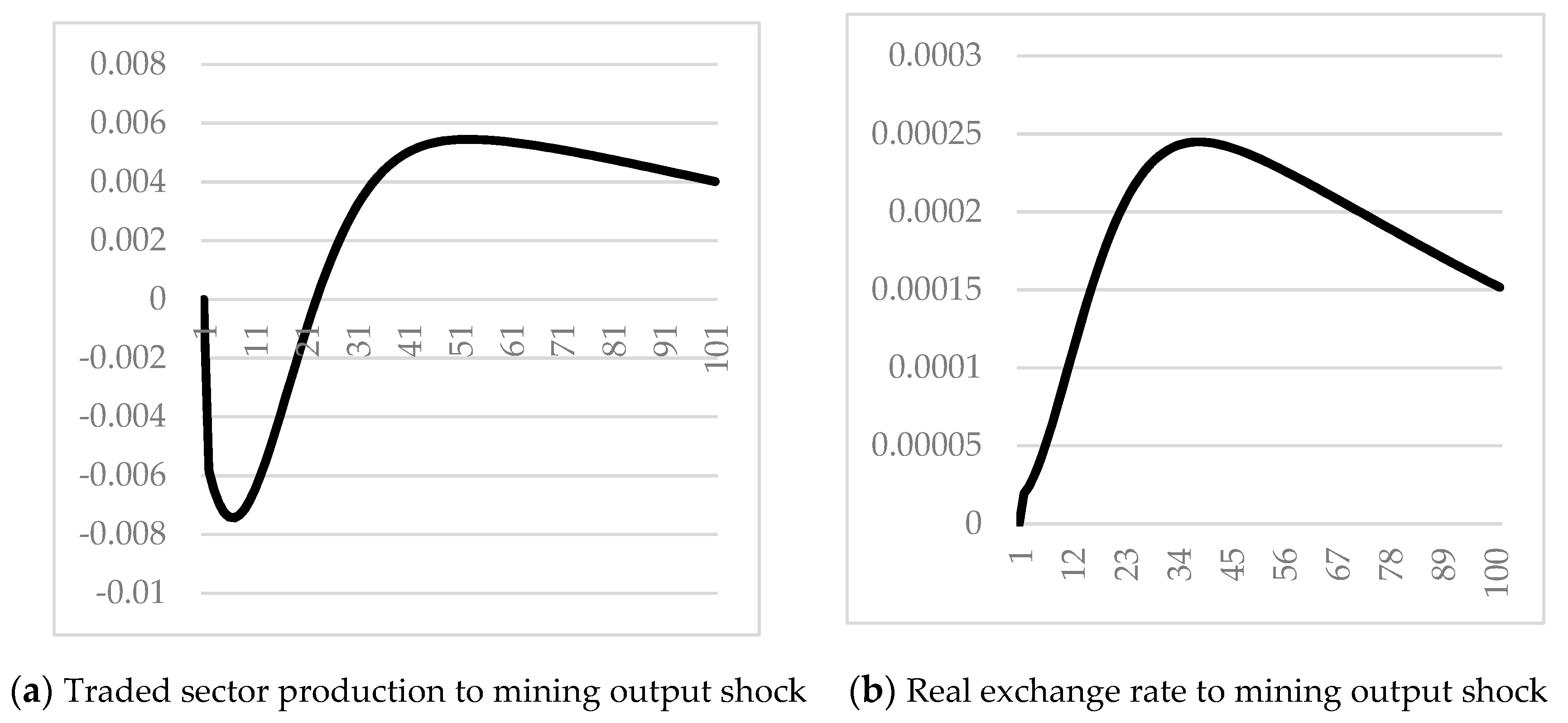
The mining sector’s shocks, both output and price, have a decreasing effect on the external debt dynamics. The mining price is higher than the output in terms of the absolute influence on external debt. Mining exports bring the country foreign currency revenue and increase its potential to repay its external debt. Even though the mining expansion has a decreasing effect on external debt, the price effect is greater than the volume effect because the increased mining production crowds out the traded sector’s output and increases the real exchange rate, as shown in Figure 3. This is the Dutch-disease effect of the mining boom [22].

Foreign interest rate shocks have a decreasing effect on external debt accumulation. The increased interest rate on foreign borrowing discourages the country from borrowing abroad because of higher debt services. Consequently, the positive foreign interest rate shock has a negative influence on the external debt dynamics of Mongolia.

4. COVID−19 Impact on External Debt of Mongolia

The earliest COVID−19 cases were reported in December 2019 in Wuhan, China; the disease has since been spreading unabated worldwide. In Mongolia, the pandemic outbreak had been mild until March 2021, thanks to early preventive measures implemented by the Government of Mongolia (GoM). However, the country’s economy was hit because of strict policy responses, including border closure and domestic lockdown, to the pandemic. The most challenging matter for Mongolia during the pandemic outbreak and the great lockdown is external debt sustainability, as the country’s external debt amount had already reached a high level before the COVID−19 shock jolted the country’s economy. Therefore, we assess the external debt dynamics of Mongolia with respect to pandemic shocks based on the estimated SOE-DSGE model constructed in this study.

The household’s preference declines because of preventive measures, whereas mining production and price falls because of border-closing policies. Similarly, the GoM approved a law on the one-time forgiveness of pension-backed debts on 10 January 2020, following the recommendations of the National Security Council of Mongolia. There were 229.4 thousand pensioners who had taken loans worth MNT 763.3 billion at the time of loan cancelation. Further, the GoM provided MNT 300,000 of support to each citizen ahead of another nationwide strict lockdown in April 2021. Cancelation of pension-backed loans and cash provision to each citizen indicates that budget spending is increasing significantly in Mongolia. Regarding the tax policy, the personal income tax and social security tax were fully or partially waived-off in 2020. Finally, the GoM declared the implementation of a fiscal stimulus package of MNT 10 trillion until 2023 to recover the economy from recession.

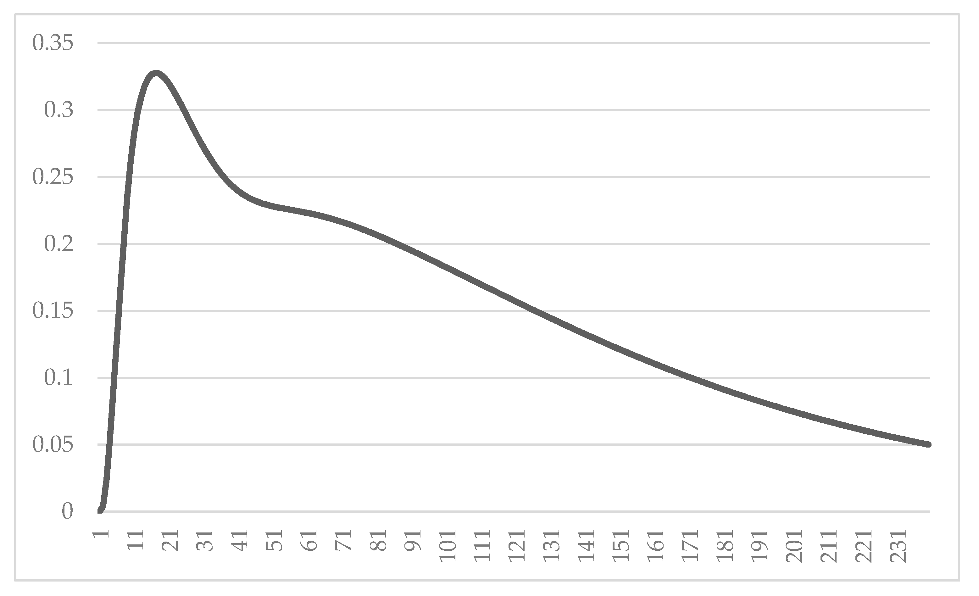
Based on real facts and policy responses, we postulated a scenario. During the COVID−19 pandemic, households’ preferences decreased by one standard deviation for four consecutive quarters, mining production and mining price declined by one standard deviation for four consecutive quarters, government spending increased by one standard deviation for eight consecutive quarters, foreign interest rate decreased by one standard deviation for four consecutive quarters, and the traded and non-traded sectors’ productivity decreased by one standard deviation for four consecutive quarters. The external debt dynamics in this scenario are shown in Figure 4.

Simulation results under the combined shocks from the COVID−19 pandemic shows that the Mongolian external debt will increase by 30% from its steady state over the next 10–28 quarters. Therefore, the country needs to pay greater attention to external debt sustainability for the next several years. In the long term, the country needs to change its basic economic structure, as the mining price and production have the highest impact on its external debt dynamics. In other words, Mongolia needs to develop the traded sector whose development lowers the external debt burden, as mentioned earlier, and decrease its dependency on the mining sector in the long term, as the mining price is volatile, which increases the economy’s vulnerability.

5. Conclusions

In this study, we constructed an SOE-DSGE model that incorporates the most pronounced features of the recent Mongolian economy, namely the external indebtedness and the mining boom. We estimated the DSGE model using the Bayesian estimation method and identified seven structural shocks: the traded and the non-traded sectors’ productivity shocks; the preference shock; the government spending shock; the foreign interest rate shock; the mining output shock; and the mining price shock. The estimation results show that the non-traded sector’s technological shock and the government spending shock have the lowest standard deviation, whereas the shocks for mining output and price have the highest standard deviation.

The traded sector’s productivity, mining price and output, and foreign interest rate have a decreasing effect on external debt, while the non-traded sector’s productivity, household preference, and government spending have an increasing impact on external debt accumulation in Mongolia. In terms of absolute influence, the mining shocks and the traded sector’s productivity shock rank the highest.

The mining price’s influence is greater than the output’s influence as the increased mining production crowd outs the traded sector’s output and increases the real exchange rate. Consequently, the country’s traded sector’s competitiveness decreases significantly, and external debt dynamics depend on the commodity price.

Further, we assess the external debt dynamics of Mongolia with respect to the pandemic shocks based on the estimated SOE-DSGE model. Under our assumed pandemic scenario, Mongolian external debt will increase by 30% from its steady-state over the next 10–28 quarters. Therefore, the country needs to pay greater attention to external debt sustainability for the next several years.

By defining the influences of the structural shocks on external debt evolution, the GoM will be able to formulate a more reasonable and long-term external debt management policy. Our recommended solution in this study is to develop the traded sector instead of the mining sector. The traded sector’s development lowers external debt burden, whereas the mining sector’s prices are extremely volatile, which may increase the economy’s vulnerability and external debt risk.

References

- Abdelaziz, H.; Rim, B.; Majdi, K. External debt, investment, and economic growth. J. Econ. Integr. 2019, 34, 725–745. [Google Scholar] [CrossRef]
- Guei, K.M. External debt and growth in emerging economies. Int. Econ. J. 2019, 33, 236–251. [Google Scholar] [CrossRef]
- Reinhart, C.M.; Rogoff, K.S. Growth in a time of debt. Am. Econ. Rev. 2010, 100, 573–578. [Google Scholar] [CrossRef] [Green Version]
- Turan, T.; Yanikkaya, H. External debt, growth and investment for developing countries: Some evidence for the debt overhang hyphothesis. Port. Econ. J. 2020, 1–23. [Google Scholar] [CrossRef]
- Li, B.G.; Gupta, P.; Yu, J. From natural resource boom to sustainable economic growth: Lessons from Mongolia. Int. Econ. 2017, 151, 7–25. [Google Scholar] [CrossRef]
- Berg, A.; Portillo, R.A.; Buffie, E.F.; Pattillo, C.A.; Zanna, L.-F. Public investment, growth, and debt sustainability: Putting together the pieces. IMF Work. Pap. 2012, 2012, 144. [Google Scholar] [CrossRef]
- Berg, A.; Portillo, R.; Yang, S.-C.S.; Zanna, L.-F. Public investment in resource-abundant developing countries. IMF Econ. Rev. 2013, 61, 92–129. [Google Scholar] [CrossRef]
- Melina, G.; Yang, S.-C.S.; Zanna, L.-F. Debt sustainability, public investment, and natural resources in developing countries: The DIGNAR model. Econ. Model. 2016, 52, 630–649. [Google Scholar] [CrossRef] [Green Version]
- Taguchi, H.; Gunbileg, G. Monetary policy rule and taylor principle in mongolia: GMM and DSGE approaches. Int. J. Financ. Stud. 2020, 8, 71. [Google Scholar] [CrossRef]
- Gali, J.; Monacelli, T. Monetary policy and exchange rate volatility in a small open economy. Rev. Econ. Stud. 2005, 72, 707–734. [Google Scholar] [CrossRef]
- Buyandelger, O.-E. Exchange Rate pass-through effect and monetary policy in mongolia: Small open economy dsge model. Procedia Econ. Financ. 2015, 26, 1185–1192. [Google Scholar] [CrossRef] [Green Version]
- Doojav, G.-O.; Batmunkh, U. Monetary and macroprudential policy in a commodity exporting economy: A structural model analysis. Cent. Bank Rev. 2018, 18, 107–128. [Google Scholar] [CrossRef]
- Doojav, G.-O.; Gantumur, M. Measuring the natural rate of interest in a commodity exporting economy: Evidence from Mongolia. Int. Econ. 2020, 161, 199–218. [Google Scholar] [CrossRef]
- Uribe, M.; Schmitt-Grohé, S. Open Economy Macroeconomics; Princeton University Press: Princeton, NJ, USA, 2017. [Google Scholar]
- Wickens, M. Macroeconomic Theory: A Dynamic General Equilibrium Approach; Princeton University Press: Princeton, NJ, USA, 2012. [Google Scholar]
- García-Cicco, J.; Pancrazi, R.; Uribe, M. Real business cycles in emerging countries? Am. Econ. Rev. 2010, 100, 2510–2531. [Google Scholar] [CrossRef] [Green Version]
- Schmitt-Grohé, S.; Uribe, M. Closing small open economy models. J. Int. Econ. 2003, 61, 163–185. [Google Scholar] [CrossRef] [Green Version]
- Schmitt-Grohé, S.; Uribe, M. How important are terms-of-trade shocks? Int. Econ. Rev. 2018, 59, 85–111. [Google Scholar] [CrossRef] [Green Version]
- Christiano, L.J.; Eichenbaum, M.; Evans, C.L. Nominal rigidities and the dynamic effects of a shock to monetary policy. J. Political Econ. 2005, 113, 1–45. [Google Scholar] [CrossRef] [Green Version]
- Hayashi, F. Tobin’s marginal q and average q: A neoclassical interpretation. Econometrica 1982, 50, 213–224. [Google Scholar] [CrossRef]
- Ahmed, Q.M.; Butt, M.S.; Alam, S.; Kazmi, A.A. Economic growth, export, and external debt causality: The case of Asian countries with comments. Pak. Dev. Rev. 2000, 39, 591–608. [Google Scholar] [CrossRef] [Green Version]
- Corden, W.M. Booming sector and Dutch disease economics: Survey and consolidation. Oxf. Econ. Pap. 1984, 36, 359–380. [Google Scholar] [CrossRef]
Figure 1.
Mongolia’s external debt ratio and mining share dynamic. Source: Author’s estimation based on publicly available data of the Bank of Mongolia, the National Statistical Office, and World Development Indicators, World Bank.
Figure 2.
External debt responses to structural shocks. Source: Author’s estimation. Note: The shocks are the positive unit standard deviations. The vertical axis represents the log deviation from the steady state.
Figure 3.
Mining output shock’s impact on the traded sector’s production and real exchange rate. Source: Author’s estimation. Note: The shocks are the positive unit standard deviations. The vertical axis represents the log deviation from the steady state.
Figure 4.
External debt deviation from its steady state under COVID−19 shocks. Source: Author’s estimation. Note: The vertical axis represents the log deviation from the steady state.