
Long-Term Evolution of the SUHI Footprint and Urban Expansion Based on a Temperature Attenuation Curve in the Yangtze River Delta Urban Agglomeration


Abstract
:1. Introduction
- (1)
- To analyze the spatiotemporal changes and influences in the YRDUA FP from 2005 to 2018.
- (2)
- To explore the developmental characteristics of the cities according to FP temperature attenuation curves.
- (3)
- To reveal the spatial overlay effect of the FP between the adjacent cities.
2. Materials and Methods
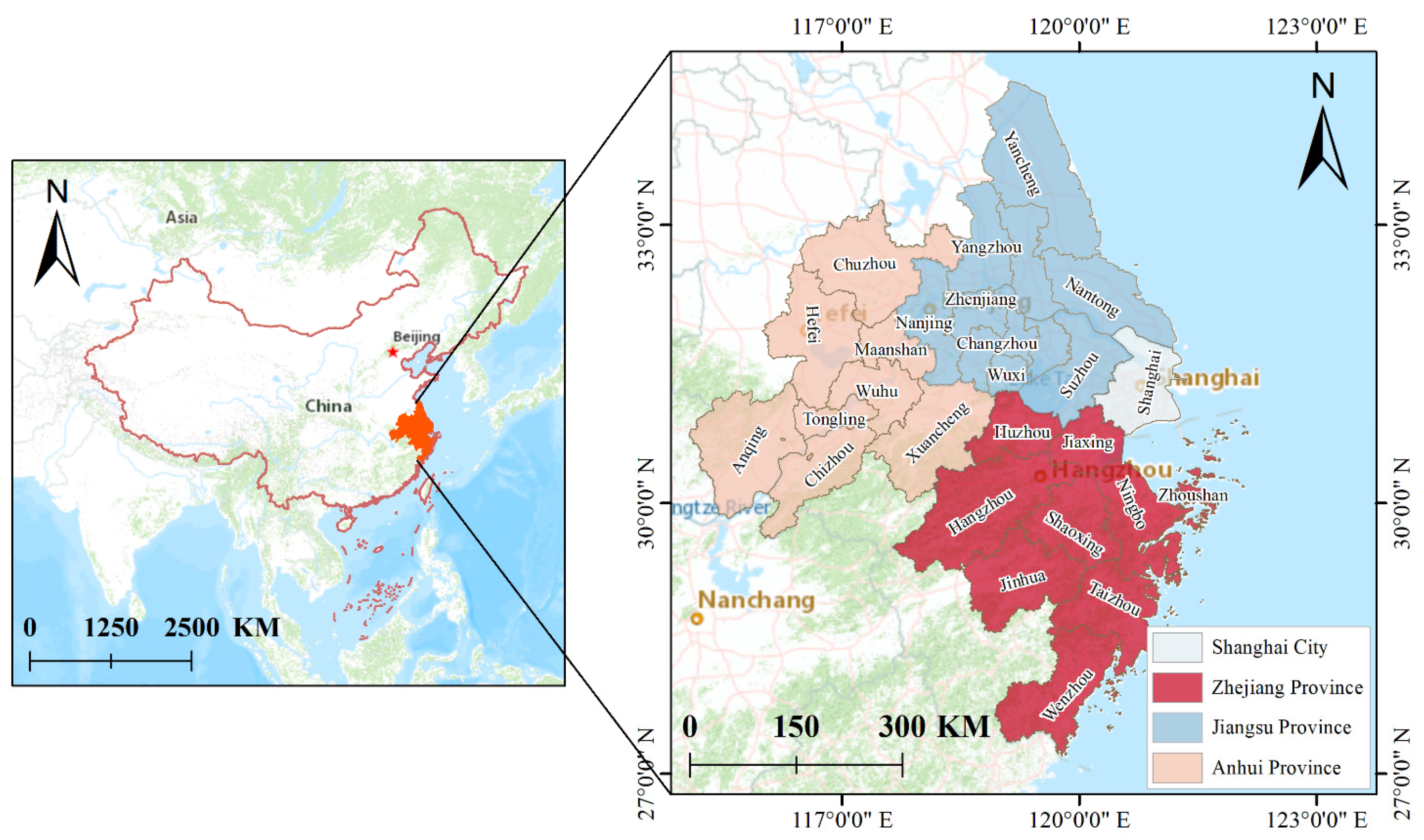
2.1. Study Area
2.2. Data
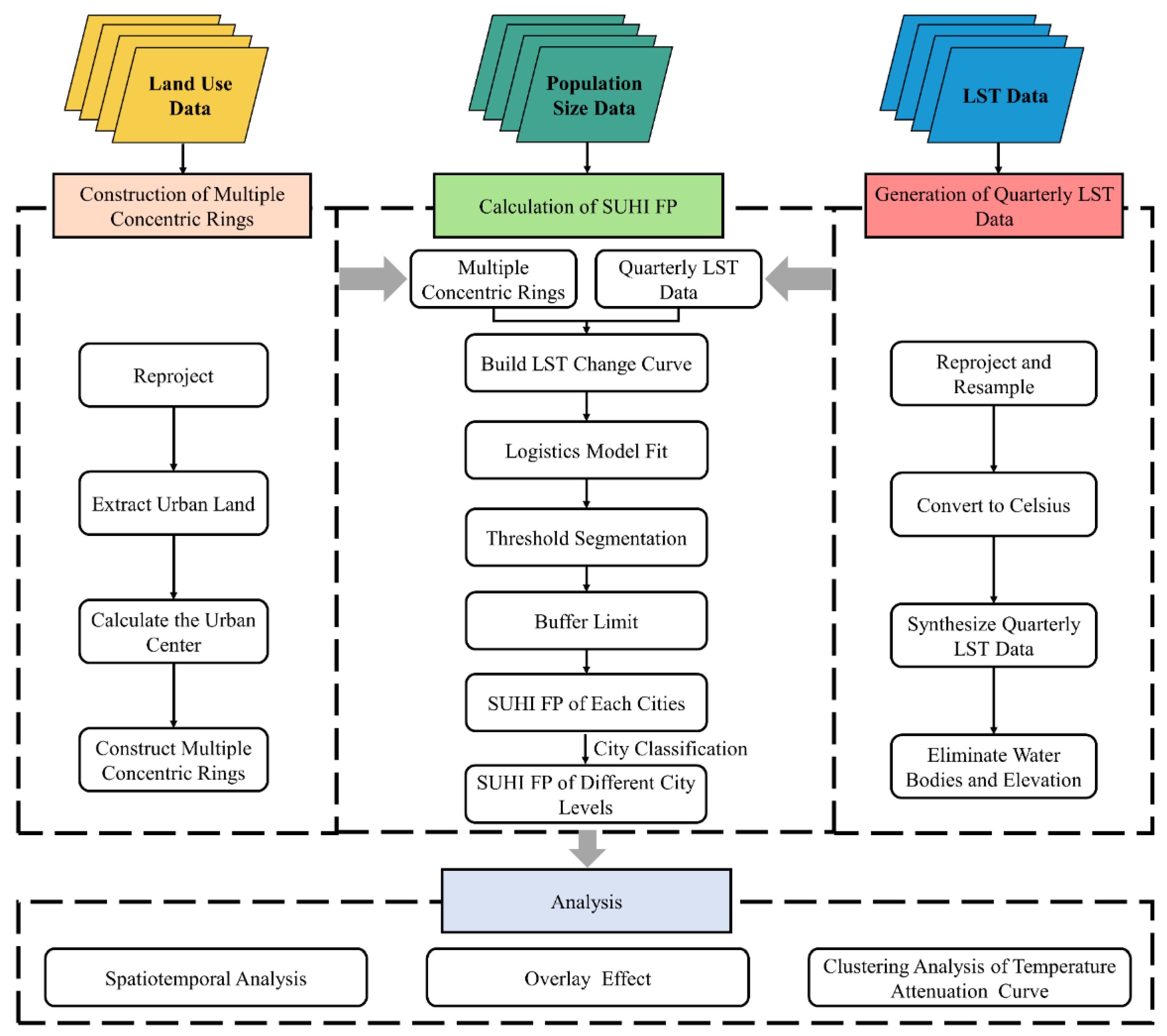
2.3. Method
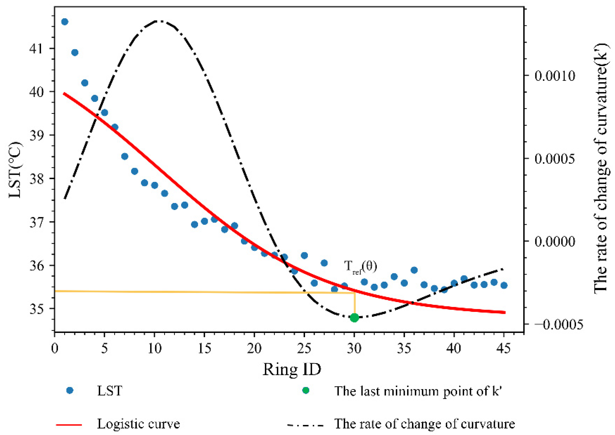
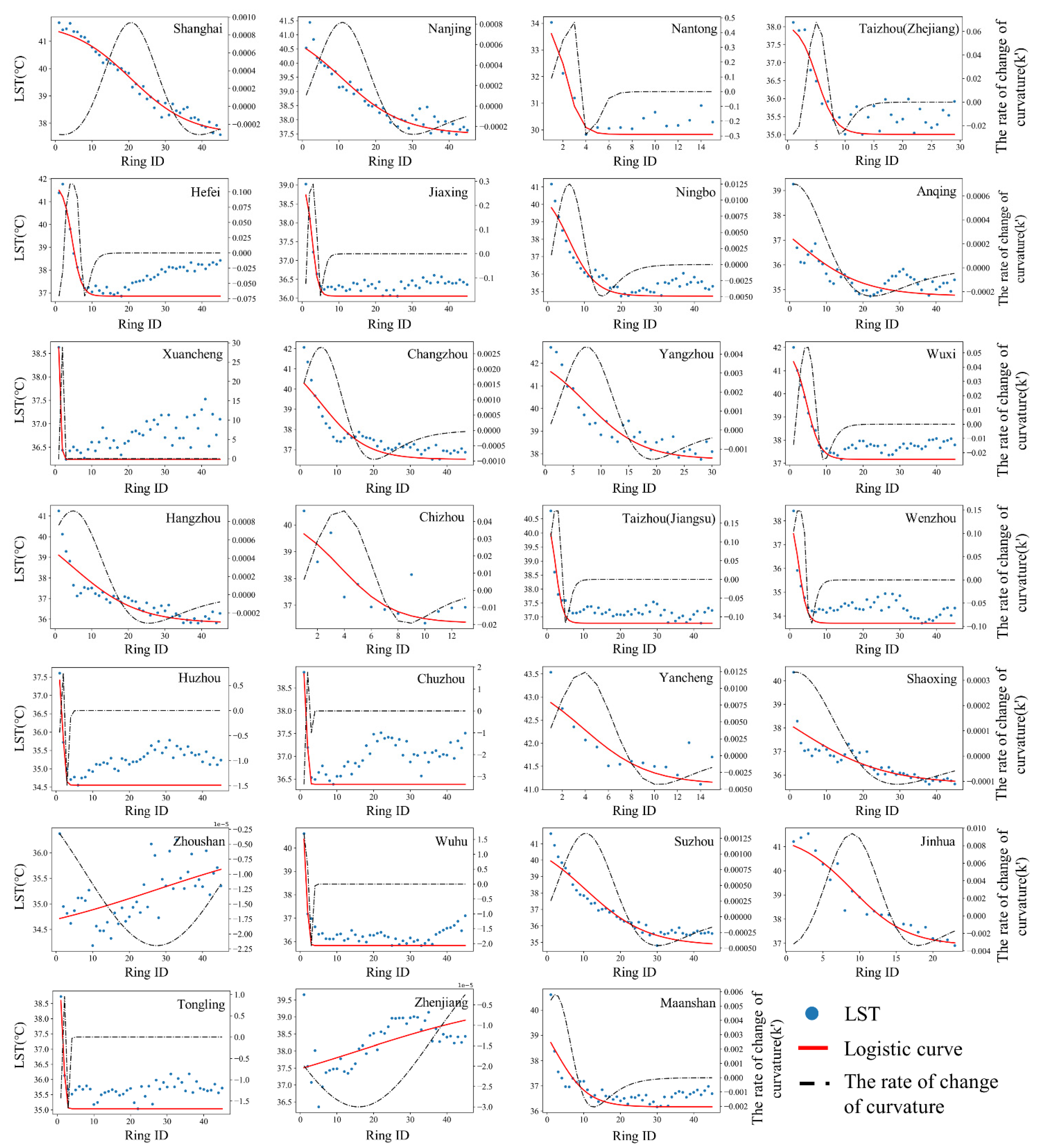
2.3.1. Calculation of the SUHI FP
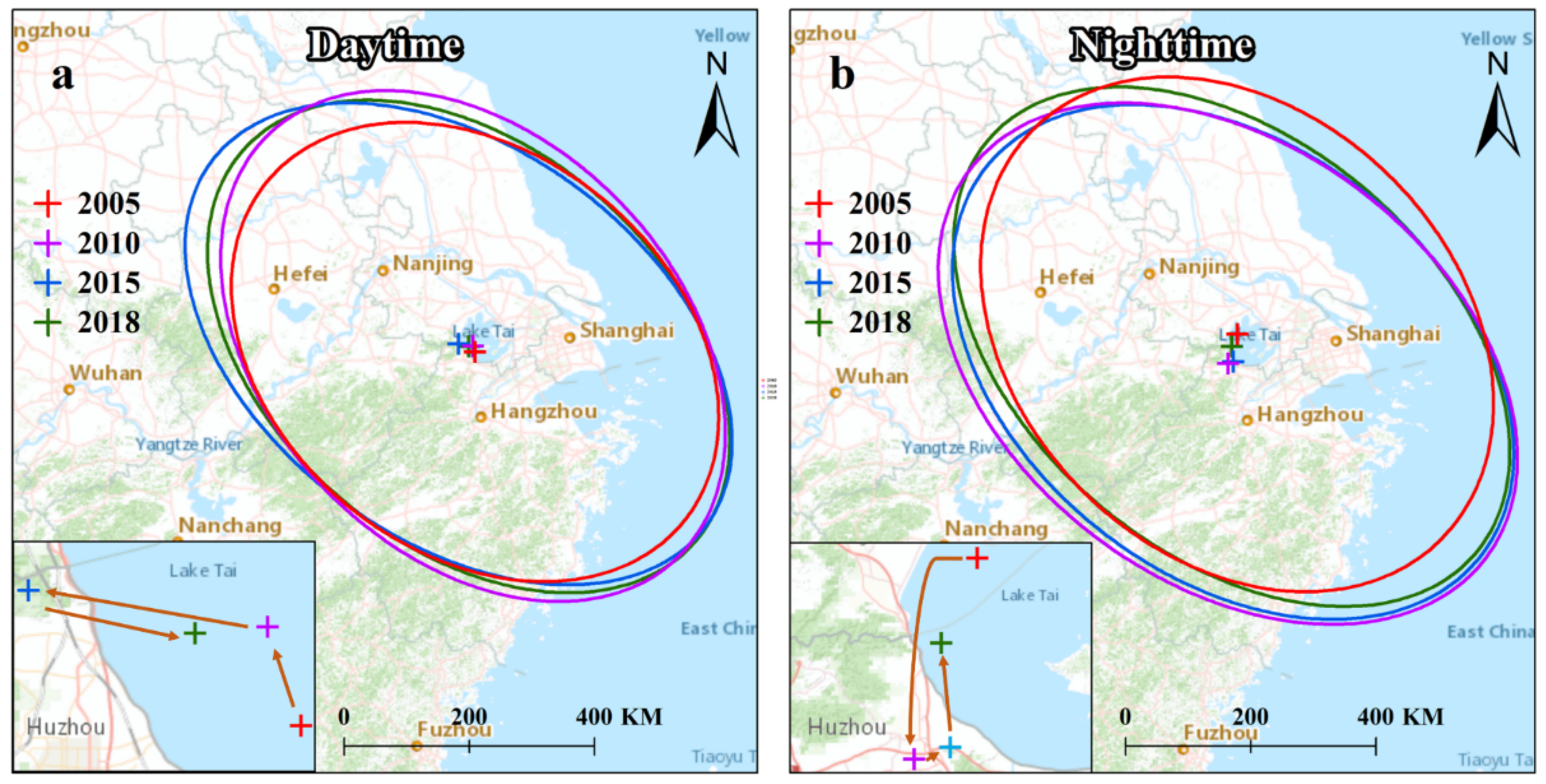
2.3.2. Standard Deviational Ellipse (SDE)
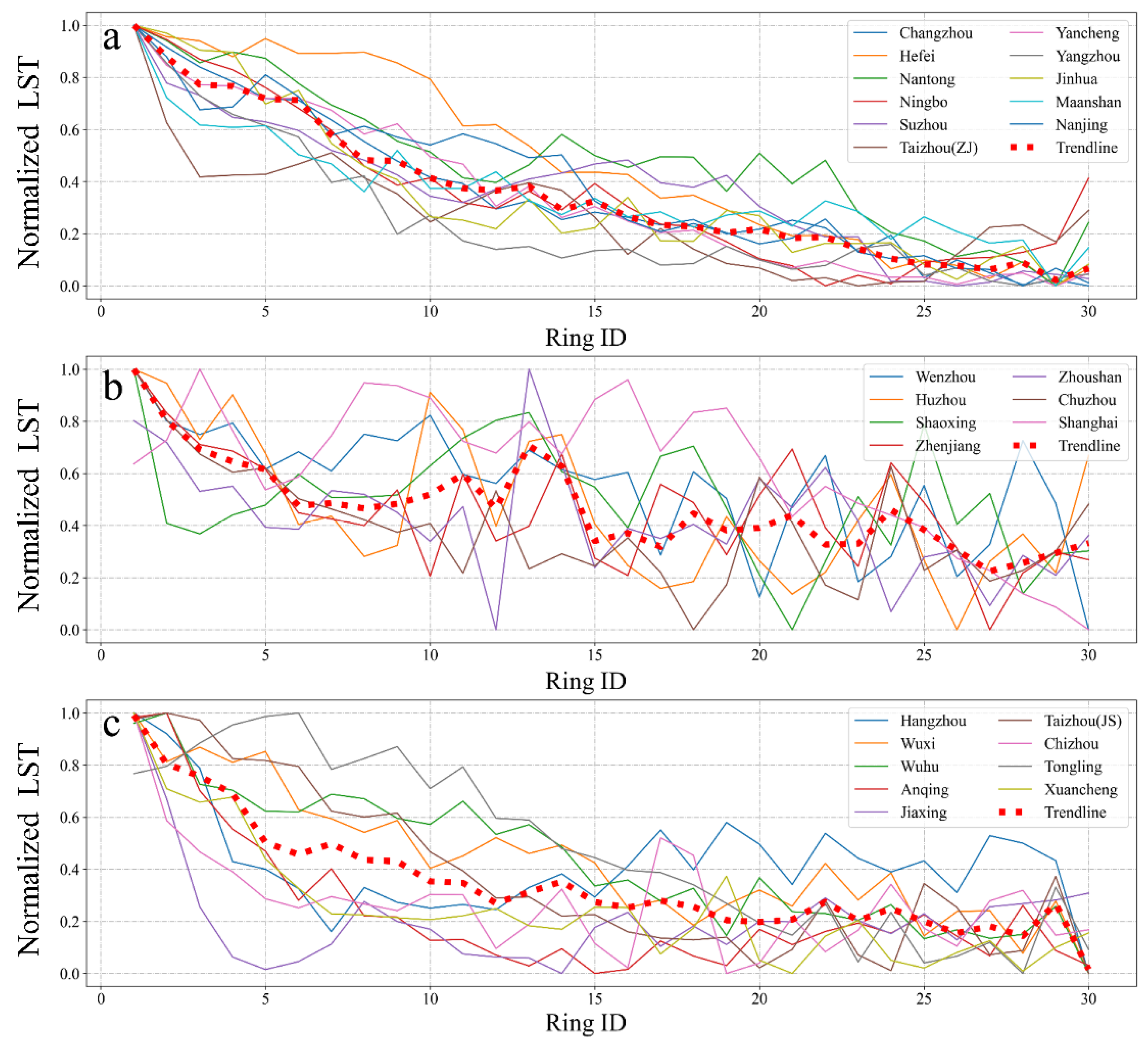
2.3.3. Clustering of UHI Attenuation Curve
3. Result
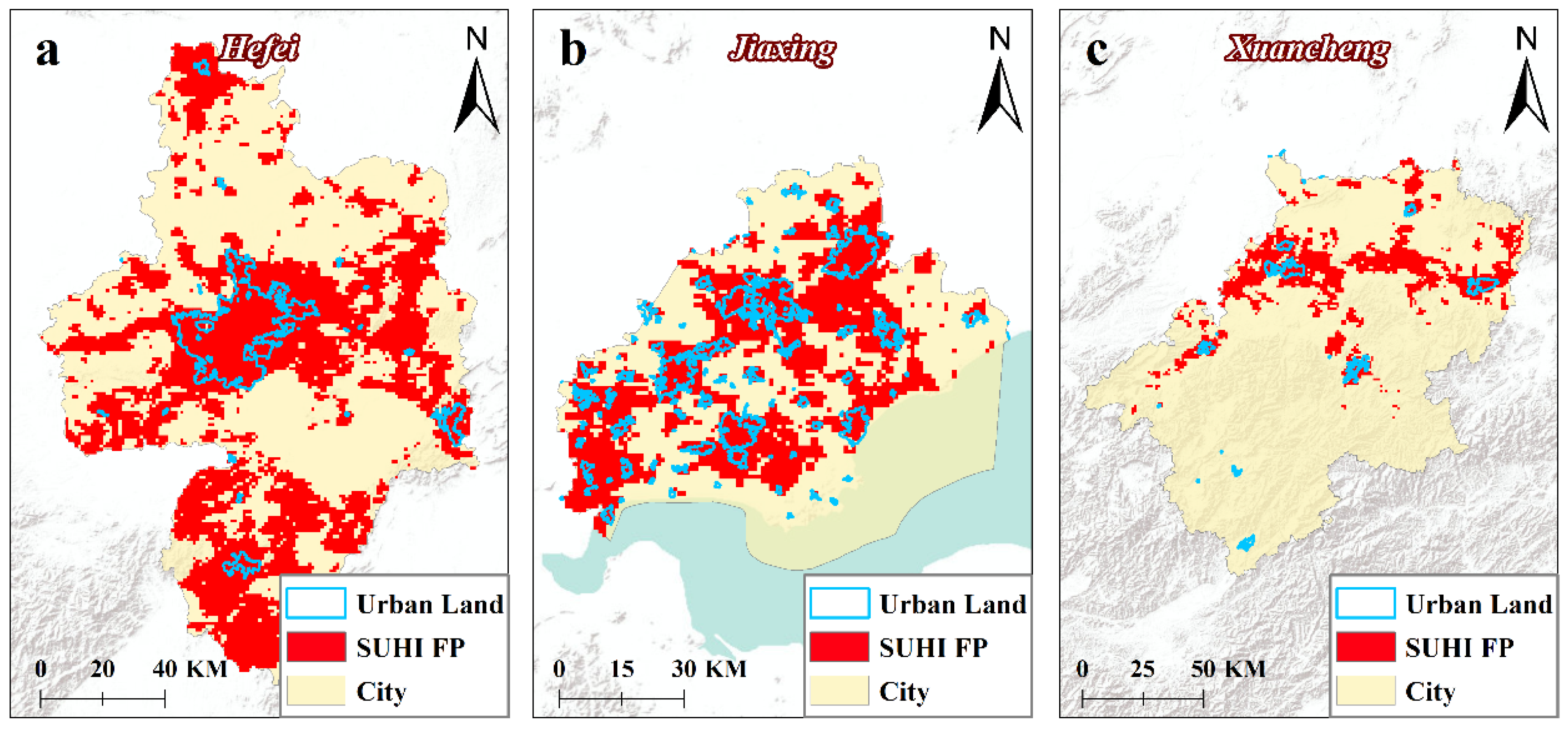
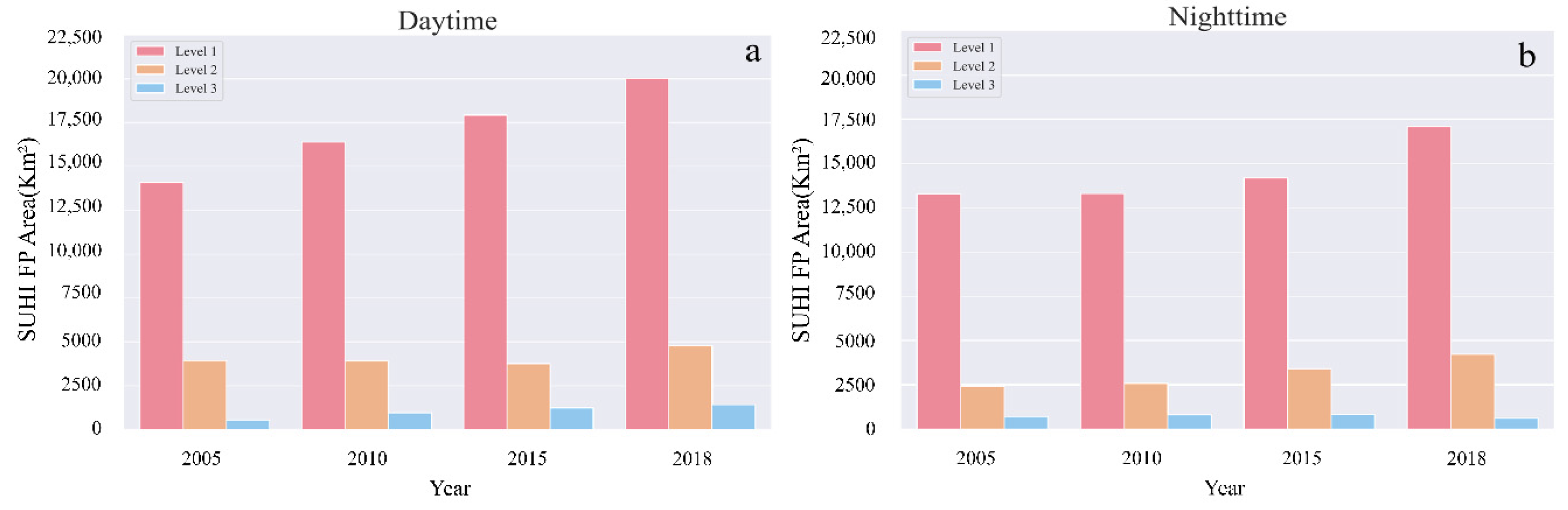
3.1. The Results of SUHI FP
3.2. Spatiotemporal Changes of SUHI FP
3.3. The Correlation between SUHI FP and Urban Development
3.4. Overlay Effect of SUHI FP
4. Discussion
4.1. Relationship between SUHI FP and Land Use
4.2. Limitations
5. Conclusions
Author Contributions
Funding
Institutional Review Board Statement
Informed Consent Statement
Data Availability Statement
Acknowledgments
Conflicts of Interest
Abbreviations
| UHI | Urban heat island |
| SUHI | Surface urban heat island |
| SUHI FP | Surface urban heat island footprint |
| YRDUA | Yangtze River Delta urban agglomeration |
| SED | Standard deviation ellipse |
| LST | Land surface temperature |
| AUHI | Atmospheric urban heat island |
| SUHII | Surface urban heat island intensity |
| RESDC | Resource and Environment Data Cloud |
| Var | Variance |
| CV | Coefficient of variation |
| SSAP | Sum of slopes of adjacent points |
References
- Madanian, M.; Soffianian, A.R.; Koupai, S.S.; Pourmanafi, S.; Momeni, M. The study of thermal pattern changes using Landsat-derived land surface temperature in the central part of Isfahan province. Sustain. Cities Soc. 2018, 39, 650–661. [Google Scholar] [CrossRef]
- Mohammad, P.; Goswami, A. A Spatio-Temporal Assessment and Prediction of Surface Urban Heat Island Intensity Using Multiple Linear Regression Techniques Over Ahmedabad City, Gujarat. J. Indian Soc. Remote Sens. 2021, 49, 1091–1108. [Google Scholar]
- Voogt, J.A.; Oke, T.R. Thermal remote sensing of urban climates. Remote Sens. Environ. 2003, 86, 370–384. [Google Scholar] [CrossRef]
- He, B.J. Potentials of meteorological characteristics and synoptic conditions to mitigate urban heat island effects. Urban Clim. 2018, 24, 26–33. [Google Scholar] [CrossRef]
- Zhou, D.; Bonafoni, S.; Zhang, L.; Wang, R. Remote sensing of the urban heat island effect in a highly populated urban agglomeration area in East China. Sci. Total Environ. 2018, 628–629, 415–429. [Google Scholar] [CrossRef]
- Lin, C.-Y.; Chen, F.; Huang, J.C.; Chen, W.-C.; Liou, Y.-A.; Chen, W.-N.; Liu, S.-C. Urban heat island effect and its impact on boundary layer development and land–sea circulation over northern Taiwan. Atmos. Environ. 2008, 42, 5635–5649. [Google Scholar] [CrossRef]
- Seto, K.C.; Golden, J.S.; Alberti, M.; Turner, B.L. Sustainability in an urbanizing planet. Proc. Natl. Acad. Sci. USA 2017, 114, 8935–8938. [Google Scholar] [CrossRef] [Green Version]
- Shahmohamadi, P.; Maulud, K.N.A.; Tawil, N.M.; Abdullah, N.A.G. The Impact of Anthropogenic Heat on Formation of Urban Heat Island and Energy Consumption Balance. Urban Stud. Res. 2011, 2011, 497524. [Google Scholar] [CrossRef] [Green Version]
- Howard, L. The Climate of London: Deduced from Meteorological Observations, Made at Different Places in the Neighborhood of the Metropolis; Harvey and Darton: London, UK, 1818. [Google Scholar]
- Mills, G. Luke Howard and the climate of London. Weather 2008, 63, 153–157. [Google Scholar] [CrossRef]
- Zhang, Q.; Xu, D.; Zhou, D.; Yang, Y.; Rogora, A. Associations between urban thermal environment and physical indicators based on meteorological data in Foshan City. Sustain. Cities Soc. 2020, 60, 102288. [Google Scholar] [CrossRef]
- Estoque, R.C.; Murayama, Y.; Myint, S.W. Effects of landscape composition and pattern on land surface temperature: An urban heat island study in the megacities of Southeast Asia. Sci. Total Environ. 2017, 577, 349–359. [Google Scholar] [CrossRef]
- Ferguson, B.; Fisher, K.; Golden, J.; Hair, L.; Haselbach, L.; Hitchcock, D.; Kaloush, K.; Pomerantz, M.; Tran, N.; Waye, D. Reducing Urban Heat Islands: Compendium of Strategies-Cool Pavements; The National Academies of Sciences, Engineering, and Medicine: Washington, DC, USA, 2008. [Google Scholar]
- Smoliak, B.V.; Snyder, P.K.; Twine, T.E.; Mykleby, P.M.; Hertel, W.F. Dense network observations of the Twin Cities canopy-layer urban heat island. J. Appl. Meteorol. Climatol. 2015, 54, 1899–1917. [Google Scholar] [CrossRef]
- Schwarz, N.; Schlink, U.; Franck, U.; Großmann, K. Relationship of land surface and air temperatures and its implications for quantifying urban heat island indicators—An application for the city of Leipzig (Germany). Ecol. Indic. 2012, 18, 693–704. [Google Scholar] [CrossRef]
- Mirzaei, P.A.; Haghighat, F. Approaches to study urban heat island–abilities and limitations. Build. Environ. 2010, 45, 2192–2201. [Google Scholar] [CrossRef]
- Deilami, K.; Kamruzzaman, M.; Liu, Y. Urban heat island effect: A systematic review of spatio-temporal factors, data, methods, and mitigation measures. Int. J. Appl. Earth Obs. Geoinf. 2018, 67, 30–42. [Google Scholar] [CrossRef]
- Weng, Q. Thermal infrared remote sensing for urban climate and environmental studies: Methods, applications, and trends. ISPRS J. Photogramm. Remote Sens. 2009, 64, 335–344. [Google Scholar] [CrossRef]
- Hu, L.; Brunsell, N.A. A new perspective to assess the urban heat island through remotely sensed atmospheric profiles. Remote Sens. Environ. 2015, 158, 393–406. [Google Scholar] [CrossRef]
- Renard, F.; Alonso, L.; Fitts, Y.; Hadjiosif, A.; Comby, J. Evaluation of the effect of urban redevelopment on surface urban heat islands. Remote Sens. 2019, 11, 299. [Google Scholar] [CrossRef] [Green Version]
- Meng, Q.; Zhang, L.; Sun, Z.; Meng, F.; Wang, L.; Sun, Y. Characterizing spatial and temporal trends of surface urban heat island effect in an urban main built-up area: A 12-year case study in Beijing, China. Remote Sens. Environ. 2018, 204, 826–837. [Google Scholar] [CrossRef]
- Deng, C.; Wu, C. BCI: A biophysical composition index for remote sensing of urban environments. Remote Sens. Environ. 2012, 127, 247–259. [Google Scholar] [CrossRef]
- Rizwan, A.M.; Dennis, L.Y.C.; Chunho, L.I.U. A review on the generation, determination and mitigation of Urban Heat Island. J. Environ. Sci. 2008, 20, 120–128. [Google Scholar] [CrossRef]
- Stewart, I.D. A systematic review and scientific critique of methodology in modern urban heat island literature. Int. J. Climatol. 2011, 31, 200–217. [Google Scholar] [CrossRef]
- Zhou, D.; Zhao, S.; Zhang, L.; Sun, G.; Liu, Y. The footprint of urban heat island effect in China. Sci. Rep. 2015, 5, 2–12. [Google Scholar] [CrossRef]
- Qiao, Z.; Wu, C.; Zhao, D.; Xu, X.; Yang, J.; Feng, L.; Sun, Z.; Liu, L. Determining the boundary and probability of surface urban heat island footprint based on a logistic model. Remote Sens. 2019, 11, 1368. [Google Scholar] [CrossRef] [Green Version]
- Wang, J.; Huang, B.; Fu, D.; Atkinson, P.M. Spatiotemporal variation in surface urban heat island intensity and associated Determinants across major Chinese cities. Remote Sens. 2015, 7, 3670–3689. [Google Scholar] [CrossRef] [Green Version]
- Li, Z.; Liu, L.; Dong, X.; Liu, J. The study of regional thermal environments in urban agglomerations using a new method based on metropolitan areas. Sci. Total Environ. 2019, 672, 370–380. [Google Scholar] [CrossRef]
- Anniballe, R.; Bonafoni, S.; Pichierri, M. Spatial and temporal trends of the surface and air heat island over Milan using MODIS data. Remote Sens. Environ. 2014, 150, 163–171. [Google Scholar] [CrossRef]
- Santamouris, M.; Paraponiaris, K.; Mihalakakou, G. Estimating the ecological footprint of the heat island effect over Athens, Greece. Clim. Chang. 2007, 80, 265–276. [Google Scholar] [CrossRef]
- Tran, H.; Uchihama, D.; Ochi, S.; Yasuoka, Y. Assessment with satellite data of the urban heat island effects in Asian mega cities. Int. J. Appl. Earth Obs. Geoinf. 2006, 8, 34–48. [Google Scholar] [CrossRef]
- Yang, Q.; Huang, X.; Tang, Q. The footprint of urban heat island effect in 302 Chinese cities: Temporal trends and associated factors. Sci. Total Environ. 2019, 655, 652–662. [Google Scholar] [CrossRef] [PubMed]
- Peng, J.; Liu, Q.; Xu, Z.; Lyu, D.; Wu, J. How to effectively mitigate urban heat island effect? A perspective of waterbody patch size threshold. Landsc. Urban Plan. 2020, 202, 103873. [Google Scholar] [CrossRef]
- Liu, Y.; Fang, X.; Xu, Y.; Zhang, S.; Luan, Q. Assessment of surface urban heat island across China’s three main urban agglomerations. Theor. Appl. Climatol. 2018, 133, 473–488. [Google Scholar] [CrossRef]
- Li, J.; Wang, F.; Fu, Y.; Guo, B.; Zhao, Y.; Yu, H. A Novel SUHI Referenced Estimation Method for Multicenters Urban Agglomeration using DMSP/OLS Nighttime Light Data. IEEE J. Sel. Top. Appl. Earth Obs. Remote Sens. 2020, 13, 1416–1425. [Google Scholar] [CrossRef]
- Huang, Q.; Lu, Y. The Effect of Urban Heat Island on Climate Warming in the Yangtze River Delta Urban Agglomeration in China. Int. J. Environ. Res. Public Heal. 2015, 12, 8773–8789. [Google Scholar] [CrossRef] [Green Version]
- Li, B.; Liu, Z.; Nan, Y.; Li, S.; Yang, Y. Comparative Analysis of Urban Heat Island Intensities in Chinese, Russian, and DPRK Regions across the Transnational Urban Agglomeration of the Tumen River in Northeast Asia. Sustainability 2018, 10, 2637. [Google Scholar] [CrossRef] [Green Version]
- Pal, S.; Xueref-Remy, I.; Ammoura, L.; Chazette, P.; Gibert, F.; Royer, P.; Dieudonné, E.; Dupont, J.-C.; Haeffelin, M.; Lac, C. Spatio-temporal variability of the atmospheric boundary layer depth over the Paris agglomeration: An assessment of the impact of the urban heat island intensity. AtmEn 2012, 63, 261–275. [Google Scholar] [CrossRef]
- Yu, Z.W.; Yao, Y.; Yang, G.; Wang, X.; Vejre, H. Strong contribution of rapid urbanization and urban agglomeration development to regional thermal environment dynamics and evolution. For. Ecol. Manag. 2019, 446, 214–225. [Google Scholar] [CrossRef]
- Chen, M.; Zhou, Y.; Hu, M.; Zhou, Y. Influence of urban scale and urban expansion on the urban heat island effect in metropolitan areas: Case study of Beijing–Tianjin–Hebei urban agglomeration. Remote Sens. 2020, 12, 3491. [Google Scholar] [CrossRef]
- Guo, A.; Yang, J.; Xiao, X.; Xia, J.; Jin, C.; Li, X. Influences of urban spatial form on urban heat island effects at the community level in China. Sustain. Cities Soc. 2020, 53, 101972. [Google Scholar] [CrossRef]
- Zhou, B.; Rybski, D.; Kropp, J.P. The role of city size and urban form in the surface urban heat island. Sci. Rep. 2017, 7, 4791. [Google Scholar] [CrossRef]
- Fang, C.; Yao, S.M.; Liu, S.H. China’s Urban Agglomeration Development Report; Science Press: Beijing, China, 2011. [Google Scholar]
- Shen, Z.; Xu, X. Influence of the Economic Efficiency of Built-Up Land (EEBL) on Urban Heat Islands (UHIs) in the Yangtze River Delta Urban Agglomeration (YRDUA). Remote Sens. 2020, 12, 3944. [Google Scholar] [CrossRef]
- Yu, Z.W.; Gao, J.; Wang, L.; Vejre, H. Suitability of regional development based on ecosystem service benefits and losses: A case study of the Yangtze River Delta urban agglomeration, China. Ecol. Indic. 2019, 107, 105579. [Google Scholar]
- Yan, J.W.; Tao, F.; Zhang, S.Q.; Lin, S.; Zhou, T. Spatiotemporal distribution characteristics and driving forces of pm2.5 in three urban agglomerations of the yangtze river economic belt. Int. J. Environ. Res. Public Health 2021, 18, 2222. [Google Scholar] [CrossRef] [PubMed]
- Du, H.; Wang, D.; Wang, Y.; Zhao, X.; Qin, F.; Jiang, H.; Cai, Y. Influences of land cover types, meteorological conditions, anthropogenic heat and urban area on surface urban heat island in the Yangtze River Delta Urban Agglomeration. Sci. Total Environ. 2016, 571, 461–470. [Google Scholar] [CrossRef]
- Cheval, S.; Dumitrescu, A. The July urban heat island of Bucharest as derived from modis images. Theor. Appl. Climatol. 2009, 96, 145–153. [Google Scholar] [CrossRef]
- Anniballe, R.; Bonafoni, S. A stable gaussian fitting procedure for the parameterization of remote sensed thermal images. Algorithms 2015, 8, 82–91. [Google Scholar] [CrossRef] [Green Version]
- Quan, J.; Chen, Y.; Zhan, W.; Wang, J.; Voogt, J.; Wang, M. Multi-temporal trajectory of the urban heat island centroid in Beijing, China based on a Gaussian volume model. Remote Sens. Environ. 2014, 149, 33–46. [Google Scholar] [CrossRef]
- Lefever, D.W. Measuring Geographic Concentration by Means of the Standard Deviational Ellipse. Am. J. Sociol. 1926, 32, 88–94. [Google Scholar] [CrossRef]
- Wang, Z.; Liu, M.; Liu, X.; Meng, Y.; Zhu, L.; Rong, Y. Spatio-temporal evolution of surface urban heat islands in the Chang-Zhu-Tan urban agglomeration. Phys. Chem. Earth 2020, 117, 102865. [Google Scholar] [CrossRef]
- Zhou, D.; Xiao, J.; Bonafoni, S.; Berger, C.; Deilami, K.; Zhou, Y.; Frolking, S.; Yao, R.; Qiao, Z.; Sobrino, J.A. Satellite remote sensing of surface urban heat islands: Progress, challenges, and perspectives. Remote Sens. 2019, 11, 48. [Google Scholar] [CrossRef] [Green Version]
- Hoan, N.T.; Liou, Y.A.; Nguyen, K.A.; Sharma, R.C.; Tran, D.P.; Liou, C.L.; Cham, D.D. Assessing the effects of land-use types in surface urban heat islands for developing comfortable living in Hanoi City. Remote Sens. 2018, 10, 1965. [Google Scholar] [CrossRef] [Green Version]


| Data | Resolution | Year | URL |
|---|---|---|---|
| MOD11A2 | 1 km | 2005, 2010, 2015, and 2018 | https://ladsweb.modaps.eosdis.nasa.gov/ |
| Land-use data | 30 m | 2005, 2010, 2015, and 2018 | http://www.resdc.cn |
| DEM | 90 m | \ | http://www.gscloud.cn |
| Population data | \ | 2005, 2010, 2015, and 2018 | http://www.mohurd.gov.cn |
| City Level | City Name |
|---|---|
| Level 1 | Shanghai, Nanjing, Hangzhou, Suzhou, Hefei, Wuxi, Ningbo, Changzhou, Wenzhou, Yancheng, Nantong, Wuhu, Yangzhou, Taizhou (ZJ) |
| Level 2 | Shaoxing, Taizhou (JS), Zhenjiang, Jinhua, Anqing, Ma’anshan, Huzhou, Zhoushan, Jiaxing |
| Level 3 | Tongling, Chuzhou, Chizhou, Xuancheng |
| Time | Year | Standard Deviation Ellipse Range (km2) | Major Axis (m) | Minor Axis (m) | Center of Gravity Coordinates | Center of Gravity Moving Distance (m) | Direction of Movement |
|---|---|---|---|---|---|---|---|
| Day | 2005 | 429,703.01 | 429,346.17 | 318,592.84 | (120°07′ E, 31°01′ N) | ||
| 2010 | 485,163.19 | 469,885.70 | 328,679.17 | (120°06′ E, 31°05′ N) | 10,044.24 | northwest | |
| 2015 | 482,801.36 | 490,496.55 | 313,337.07 | (119°53′ E, 31°07′ N) | 23,257.10 | northwest | |
| 2018 | 475,779.29 | 477,480.21 | 317,196.35 | (120°02′ E, 31°05′ N) | 16,559.18 | southeast | |
| Night | 2005 | 509,465.55 | 3,650,919.71 | 461,815.62 | (120°03′ E, 31°16′ N) | ||
| 2010 | 563,916.79 | 515,661.74 | 348,118.94 | (119°56′ E, 30°54′ N) | 49,089.05 | southwest | |
| 2015 | 540,783.54 | 502,414.05 | 342,640.69 | (120°00′ E, 30°55′ N) | 8815.38 | northeast | |
| 2018 | 528,632.51 | 510,257.64 | 32,9794.37 | (119°59′ E, 31°07′ N) | 24,417.73 | northwest |
| City | Population Size Category | Clustering Category | City | Population Size Category | Clustering Category |
|---|---|---|---|---|---|
| Changzhou | 1 | 1 | Anqing | 2 | 3 |
| Hangzhou | 1 | 3 | Huzhou | 2 | 2 |
| Hefei | 1 | 1 | Jiaxing | 2 | 3 |
| Nanjing | 1 | 1 | Jinhua | 2 | 1 |
| Nantong | 1 | 1 | Ma’anshan | 2 | 1 |
| Ningbo | 1 | 1 | Shaoxing | 2 | 2 |
| Shanghai | 1 | 3 | Taizhou (JS) | 2 | 3 |
| Suzhou | 1 | 1 | Zhenjiang | 2 | 2 |
| Taizhou (ZJ) | 1 | 1 | Zhoushan | 2 | 2 |
| Wenzhou | 1 | 2 | Chizhou | 3 | 3 |
| Wuxi | 1 | 3 | Chuzhou | 3 | 2 |
| Wuhu | 1 | 3 | Tongling | 3 | 3 |
| Yancheng | 1 | 1 | Xuancheng | 3 | 3 |
| Yangzhou | 1 | 1 |
| Level | Type | Daytime | Nighttime | ||||||
|---|---|---|---|---|---|---|---|---|---|
| 2005 | 2010 | 2015 | 2018 | 2005 | 2010 | 2015 | 2018 | ||
| Level 1 | Farmland | 51.676 | 42.715 | 39.884 | 37.592 | 53.413 | 39.689 | 37.148 | 35.025 |
| Forest | 4.547 | 5.386 | 3.589 | 3.66 | 4.985 | 4.662 | 3.971 | 3.75 | |
| Grassland | 0.146 | 0.142 | 0.124 | 0.359 | 0.306 | 0.222 | 0.152 | 0.719 | |
| Water | 2.946 | 3.355 | 2.096 | 2.85 | 4.395 | 4.031 | 2.726 | 4.398 | |
| Built-up land | 40.669 | 48.22 | 54.266 | 55.482 | 36.873 | 51.192 | 55.98 | 55.803 | |
| Unused lands | 0.018 | 0.095 | 0.041 | 0.058 | 0.028 | 0.076 | 0.021 | 0.304 | |
| Level 2 | Farmland | 60.199 | 50.941 | 47.785 | 47.067 | 49.941 | 44.412 | 46.536 | 45.358 |
| Forest | 7.425 | 10.879 | 7.323 | 4.931 | 6.981 | 5.913 | 6.478 | 3.675 | |
| Grassland | 1.862 | 1.181 | 1.338 | 0.967 | 2.901 | 3.1 | 2.308 | 2.325 | |
| Water | 5.879 | 6.358 | 3.789 | 4.222 | 10.062 | 11.487 | 6.319 | 9.896 | |
| Built-up land | 22.99 | 30.632 | 39.724 | 42.761 | 30.11 | 35.083 | 38.318 | 38.689 | |
| Unused lands | 0.005 | 0.009 | 0.043 | 0.053 | 0 | 0.004 | 0.039 | 0.059 | |
| Level 3 | Farmland | 56.036 | 52.058 | 47.783 | 53.314 | 49.948 | 45.746 | 46.536 | 45.358 |
| Forest | 9.136 | 9.36 | 12.801 | 8.167 | 9.821 | 8.46 | 12.729 | 8.439 | |
| Grassland | 5.342 | 5.487 | 5.892 | 5.434 | 5.213 | 5.597 | 4.28 | 4.584 | |
| Water | 7.692 | 5.829 | 2.609 | 4.17 | 8.869 | 7.51 | 5.94 | 8.017 | |
| Built-up land | 21.795 | 27.177 | 31.870 | 28.375 | 17.927 | 28.473 | 26.716 | 32.44 | |
| Unused lands | 0 | 0.089 | 0.044 | 0.539 | 0 | 0.012 | 0.046 | 0.773 | |
Publisher’s Note: MDPI stays neutral with regard to jurisdictional claims in published maps and institutional affiliations. |
© 2021 by the authors. Licensee MDPI, Basel, Switzerland. This article is an open access article distributed under the terms and conditions of the Creative Commons Attribution (CC BY) license (https://creativecommons.org/licenses/by/4.0/).
Share and Cite
Tao, F.; Hu, Y.; Tang, G.; Zhou, T. Long-Term Evolution of the SUHI Footprint and Urban Expansion Based on a Temperature Attenuation Curve in the Yangtze River Delta Urban Agglomeration. Sustainability 2021, 13, 8530. https://doi.org/10.3390/su13158530
Tao F, Hu Y, Tang G, Zhou T. Long-Term Evolution of the SUHI Footprint and Urban Expansion Based on a Temperature Attenuation Curve in the Yangtze River Delta Urban Agglomeration. Sustainability. 2021; 13(15):8530. https://doi.org/10.3390/su13158530
Chicago/Turabian StyleTao, Fei, Yuchen Hu, Guoan Tang, and Tong Zhou. 2021. "Long-Term Evolution of the SUHI Footprint and Urban Expansion Based on a Temperature Attenuation Curve in the Yangtze River Delta Urban Agglomeration" Sustainability 13, no. 15: 8530. https://doi.org/10.3390/su13158530