
CFD Prediction of Performance of Wind Turbines Integrated in the Existing Civil Infrastructure

1
Faculty of Science, Engineering and Computing, Kingston University, London SW15 3DW, UK
2
Institute of Hydrodynamics and Control Processes, St Petersburg State Marine Technical University, 190121 St. Petersburg, Russia
*
Author to whom correspondence should be addressed.
Sustainability 2021, 13(15), 8514; https://doi.org/10.3390/su13158514
Submission received: 15 June 2021
/
Revised: 20 July 2021
/
Accepted: 27 July 2021
/
Published: 30 July 2021
(This article belongs to the Special Issue Design and Optimization of Renewable Energy Systems)
Abstract
:Power generation from wind energy is almost entirely performed in rural locations or at sea, and very little attention has been given to the use of wind turbines in urban locations. Since the re-emergence of wind turbines, the majority of their applications are in large commercial wind farms in rural areas or out at sea, and there is an increasing focus on the use of wind turbines within an urban environment possibly using existing structures, such as bridges and viaducts. There are very few existing buildings which have been designed from the ground-up to include wind turbines in the structure. In order to estimate the wind resources and the performance of a turbine at a particular site, a CFD model is designed and CFD calculations are performed. In order to simplify the modelling of a wind turbine actuator, disc theory is applied. Actuator disc theory is used, as it allows the aerodynamic behaviour of a wind turbine to be analyzed by just considering the energy extraction process without a specific wind turbine design. The power output of wind turbines installed beneath an already existing civil infrastructure is determined and analyzed.
1. Introduction
As conventional fossil fuel supplies diminish and cause concern over environmental pollution rises, renewable energy sources have proved more attractive, such as wind, solar, or geothermal sources [1]. The attractiveness of renewable sources has increased due to the increase in costs associated with fossil fuel consumption and the growing awareness and public desire for green methods of energy production. They also allow for the possibility of effective de-centralization of energy production and an increase in self-sufficiency, which is particularly attractive for remote populations. The method of renewable energy production used varies across the globe in order to utilize the most effective method for the specific location [2].
Integration of wind turbines in buildings has been studied for many years and is expected to be well-developed in the near future [3]. Turbines are located in high points of the building in order to take advantages of higher speeds. There are existing buildings which have been designed from the ground-up to include wind turbines in the structure, although more are proposed in the future.
The world’s leading example of a building-integrated wind energy conversion system is probably the 50-storey, 240 m high Bahrain World Trade Center (Manama, Bahrain), which uses three large turbines of 29 m diameter each between two towers to generate approximately 1100–1300 MWh per year. These two towers are shaped specifically to accelerate and direct the air flow to the fixed direction turbines, allowing them to operate between 270 and 360 degrees, although they are restricted to operate only between 285 and 345 degrees to ensure no damage is caused [4]. Fixed-direction turbines have been used in order to ease the integration into the building, although this restricts the amount of time that they can operate; however, the shape of the building which faces the dominating prevailing wind is used to overcome this restriction. Results of the Computational Fluid Dynamics (CFD) analysis performed in [4] show how the towers create an S-shaped streamline through the centre.
One of the world’s first buildings with a fully integrated wind turbine system is the 43 storey Strata building located in Elephant and Castle (London, UK), which was completed in 2010. At the top of the tower, three 9 m diameter Horizontal Axis Wind Turbines (HAWTs) are located, which are enclosed in order to increase their efficiency through the venture effect. They provide 8% of the building’s energy needs and exceed UK building regulations by 13%. The three 9 m turbines are rated at 19 kW and expected to produce 50 MWh each year.
An example of a way to integrate wind power generation into existing structures is the addition of a wind turbine to the Bolte Bridge in Melbourne (Australia), as proposed in [5]. The Bolte Bridge is in a prize location to take advantage of wind energy generation in an urban environment, as it is unobstructed by the surrounding buildings. This idea has not been considered or developed into a viable proposition.
Two small turbines have been added to the top of the EMSD Headquarters Building in Hong Kong, which are a 1 kW HAWT and a 1.5 kW Vertical Axis Wind Turbine (VAWT). These are mainly to provide operational experience and demonstrate the application of small wind turbines rather than as an effective energy generation proposal.
The Oklahoma Medical Research Facility (Oklahoma City, OK, USA) has had an array of VAWTs included into the roof of a new research tower and was opened in 2012. This is currently the largest building-integrated wind turbine system in the US, with 18 turbines rated at 4.5 kW each produced by Venger Wind.
Obviously, not all proposed ideas are followed through—for example, the Freedom Tower in New York was at one stage supposed to include the world’s first urban wind farm; however, wind energy is now produced for the tower at a different location.
The Zona Eylica Canaria Socied ad Anynima (ZECSA) is a Spanish company that looks to promote the use of renewable energy generation, particularly in an urban environment for the Plan for Exploitation of Public Infrastructures for Renewable Energies (PAINPER in Spanish initials). The Canary Islands possess optimum conditions for large-scale exploitation of renewable energies, especially wind energy. The Canaries are situated at a point where Trade Winds, constant east winds, make these islands an interesting area for the development of wind infrastructures. Along with these general currents, there exist local winds owing to differential warming, sea breeze, or vale-mountain flows. In addition, particular orographic conditions of terrains would affect local winds and create small locations with good conditions for wind power.
ZESCA proposed a study into energy production using wind turbines implemented into the structure of the Juncal Viaduct in Galdar, Gran Canaria. This viaduct is part of the dual carriageway which connects the three main populations of Santa Maria de Guia, Goldar and Agaete. The designed structure, with a direction of North–South, had a span of 250 m long and a height of 63 m, with a slope of 0.52%. The Juncal Viaduct has a platform with a total length of 11 m and a camber of 1.42%. It is supported by two doubled pillars of 46.60 m and 33.80 m, respectively. The energy production from the wind farm would not be very high due to conditions of the location, characterized by geographical and spacing conditions. It is not possible to choose an ideal site for the wind turbine as it must be adapted to the existing conditions.
Different arrangements of various sizes of HAWTs to find the most effective arrangement were used in [6]. In this location, the air is channelled along a valley to the wind turbines, and this would increase the turbulence of the air reaching the wind turbines. Due to this, it is possible that the use of VAWTs would be more suited to this particular application as they out-perform HAWTs in turbulent airflow [7]. The actuator disc theory and analytical wake model were applied in [8] to assess power output generated by the wind farm.
The study presents an assessment of the expected power output from a wind turbine placed in an existing viaduct, and describes CFD results used to model the wind flow through a turbine for a range of resistances of disc representing turbine rotor. The use of VAWTs to HAWTs at this specific location is compared against the results computed in [6] for different configurations based on HAWTs.
During the research of [6], different arrangements of various sizes of HAWTs have been used to find the most effective arrangement. In this location, the air is channelled along a valley to the wind turbines, and this would increase the turbulence of the air reaching the wind turbines. Due to this, it is possible that the use of VAWTs would be more suited to this particular application, as they out-perform HAWTs in turbulent airflow. This study attempts to re-create the CFD model created during the study in [6] in order to compare the use of VAWTs to HAWTs at this specific location. The methodology exploitees the actuator disc theory and CFD calculations to find the maximum power output of the wind farm.
2. Actuator Disc
Actuator disc theory has been largely used in wind turbine studies. In fact, in order to analyze the wind flow quantitatively, a resistance coefficient is introduced in the actuator disc. This would give the disc a porosity which would diffuse the wind incident in its upstream surface.
A porous disc was applied in [9] to analyze the effect of turbine resistance and shrouding in order to calculate the maximum power extracted from a given rotor diameter and from a given area of stream. The same procedure was used in [10] to study the performance of a building-mounted ducted cross-flow wind turbine. The theory of actuator disc in the study of wake flow in tidal turbines in both numerical and experimental procedures was introduced in [11]. This study came to the conclusion that a porous disc instead of the real blade model could be a validated and accurate way for tidal turbines modelling. The main reason for using an actuator disc is its more simple design which avoids complex meshing, which would require high computational effort.
A CFD package to study the behavior of tidal energy converters was used in [12]. A simplified computational domain was designed to locate the converter with the aim of decreasing computational times. The study confirms again that actuator disc models offer an economically viable analysis tool in terms of mesh size and solution timescales. In fact, as mesh size is reduced, generation time for a turbine model would be reduced as well. Simulation of actuator discs in the study of wind flows is a potentially economically viable analysis tool [13].
In order to use actuator disc theory, a frozen body in disc shape of the correct diameter for the chosen wind turbine is created. The disc is then set as a porous domain consisting of both the fluid (air is treated as ideal gas) and the solid (steel). The resistance of the blades to the flow is given in terms or porosity for the disc with a value from 0 to 1, where 0 represents a solid wall and a value of 1 gives no resistance. For this study, the disc representing the turbine is given a porosity of 9 or 90%, this means that there is only a 10% reduction in the available flow area.
In order to measure the power generated by the turbine, the momentum extraction is to be simulated. This is done by giving the disc a thrust term opposing the normal flow. This loss model is defined by a liner or quadratic loss coefficient which takes into account the pressure gradient across the disc. In this case, a quadratic loss coefficient is used, ranging from 0 to 8 kg/m, allowing the pressure drop to be measured for a variety of different turbine characteristics. The power is calculated by
where and are the static pressures immediately upstream and downstream of the rotor, respectively, u is the one-dimensional wind speed immediately upstream of the rotor, and is the air density, is the efficiency of the turbine, and A is the flow area. The disc has a drag coefficient, k, giving the relationship between the pressure drop across the disc to the induced velocity immediately upstream of the disc [14].
3. Configurations of Wind Turbines
Initially, a full-size domain of the valley and the surrounding area as was done in the [6] study was created and meshed (Figure 1a). In order to reduce the processing requirements, a much smaller and less complicated domain was required. This was done by taking the straight section of the valley where the viaduct is located (Figure 1b). Dimension restrictions due to the presence of the irregular terrain, pillars, and viaduct platform are taken into account. Distance between pillars is 119.25 m, while maximum height between the ground and bottom surface of the viaduct is 60.90 m. Altogether it makes a total available surface of approximately 5900 m. However, due to the geometric characteristics of wind turbines, not all the surface available would be occupied.
Three different models are used in CFD calculations. The first model, single HAWT, is the same as the one used in the [6] study. It includes a single 46 m diameter HAWT mounted below the viaduct with an area of 1661.9 m (Figure 2a). The second model, single VAWT, is a large VAWT mounted below the viaduct in a similar manner to the previous HAWT. It is 44 m tall by 36 m wide with a total area of 1584 m (Figure 2b). In order to take advantage of different wind directions and the higher wind speeds above the viaduct, the third model uses two VAWTs mounted on top of the viaduct supports, above the roadway. They both measure 35 m tall by 20 m wide and each have an area of 700 m, giving a combined area of 1400 m (Figure 2c).
CFD models used in the study are similar to those designed in [6]. An unstructured finite volume incompressible solver is used to carry out CFD calculations [15]. They are based on Reynolds-averaged Navier–Stokes (RANS) equations and Shear Stress Transport (SST) turbulence model [16]. Details of the numerical methods and finite-difference schemes are provided in [17,18].
4. Wind Data
In order to provide comparable results to those in the study performed in [6], the same wind data are used. The raw data were taken from the IDAE (Instituto para la Diversificacion Ahorro de Energia, atlaseolico.idae.es/meteosim) and the ITC (Instituto Tecnologico de Canarias). Figure 3 shows the wind rose at 80 m at point (432450, 3109650) taken from IDEA [6]. It shows the predominant wind direction is towards the north-east with a 30% frequency, and a 25% frequency in the east-north-east direction.
Taking the wind direction to be north-east, the ITC and IDEA wind data at a variety of different heights are given in Table 1 and Table 2, where z is the height, v is the wind speed, c is the form factor, and C is the scale factor. Wind data provided by IDAE are more complete as Weibull constant, C, has been added, which is useful for the calculation of the wind resource at different speeds. Using data given by ITC, the Weibull distribution for the wind inlet at 40 m high are calculated.
Wind frequency is calculated by the equation proposed in [19]. To calculate the wind height variation in a short-term period (minutes and hours), the model proposed in [20] is applied. These equations contain a number of constants depending on wind speed and surface roughness [21]. The chosen roughness length is fixed at 0.1 m as the assessed area, due to the absence of woods and the presence of only a few trees and crops [22].
5. Domain
In order to produce the most accurate results, it is important to use a domain size which has no effect on the simulations (the simulation is independent of the domain size). To reduce the computing time required to process a problem, the smallest possible domain size which still allows the simulation to be independent should be used. As one dimension, the length of the valley, has been set by the physical geometry, only the domain height and width can be varied. Each domain gets progressively larger until no change is recorded in the results. The smallest domain that allows for a domain-independent solution is used in order to speed-up the computational time.
The length and width of each domain used in CFD calculations are presented in Table 3. The computed results are shown in Table 4.
The size of the domain has a large impact on the pressures recorded and the induced velocity. For the first two domain (domains 1 and 2) sizes, the percentage difference was over acceptable limits at 3.93% and 2.46% for and 4.64% for , meaning they were not independent. By domain three, much smaller percentage differences were calculated with the exception of and the generated power at 2.07% and 2.12%, respectively. After domain 3, all percentage differences fall below 1%; hence, domain 3 is used in order to reduce the processing time, whilst allowing for domain independence. Plots of this data are given in Figure 4.
6. Mesh
An unstructured hybrid mesh has been created using pyramid and tetrahedral elements and an inflation layer over the ground of the model and around the turbine. In order to reduce the processing time, the mesh is biased, allowing it to be finer towards the regions expected to undergo the greatest changes in wind velocity and pressure gradient, such as the viaduct edges, bridge, and the porous disc, whilst also allowing the mesh to be coarser in the outlying regions.
Wall functions are used to simulate the mean wind profile and the turbulent kinetic energy, as this allows further simplification of the mesh and simulation. As a result, a yplus coordinate of between 30 to 300 is used, as the first node distance does not need to intercept the viscous sub-layer. At 10% stream-wise length, using an initial velocity of 4 m/s from the ITC data, the Reynolds number is , and the flow is turbulent. The first node distance is calculated as
As a hybrid mesh and inflation layer are being used, it is important that the inflation layer extends above the maximum boundary layer thickness. The boundary layer thickness at a 100% characteristic length is m, where .
The inflation uses 39 layers with a growth rate kept at 20% to ensure a smooth transition. The inflation layer first node distance is 0.0165 m and the final node is at 16.841 m, ensuring that the 100% boundary layer thickness of 7.52 m is included. The same method is used to calculate the inflation layer for each of the different turbine models.
To ensure that the most accurate result is achieved using the set-up chosen, the resolution of the mesh should be increased to check that the element size does not influence the results (mesh-independent solution). It then allows the smallest usable mesh to be identified, saving on processing time. To check the independence, five different values are monitored using configuration A from [6]. This allows the results to be validated against their findings: pressure immediately before the turbine, ; pressure immediately after the turbine, ; induced velocity, ; mass flow rate through the turbine, ; power generated by the turbine at 8 kg/m, P. Monitoring these values allows the effect of increasing the mesh resolution to be studied and comparisons between each resolution step to be made. If the difference between each resolution is less than 2% for consecutive meshes, then the study is independent. The coarsest resolution which displays this relationship with the following meshes are used. The percentage difference between each mesh is calculated by
Number of cells and nodes used in CFD calculations is presented in Table 5. The maximum values of the yplus coordinate are also included to provide a better insight into details of CFD simulations. Figure 5 shows the typical mesh and how the inflation is observed in one of the configurations (single HAWT) used in CFD calculations. To minimize computational time, the mesh is predefined to be coarser in the region of the flow domain and more refined in the porous flow domain to capture sudden changes of the wind velocity.
The results computed are shown in Table 6. It shows that there is a small difference in the pressures and the mass flow rates through the wind turbine between all six meshes tested. There is a range of 0.01% to 0.40% for , 0.47% to 1.11% for and 0.06% to 0.31% for the mass flow rate. The velocity and power generated, however, change significantly for each increase in mesh resolution, further increases were not possible due to a restriction on the processing power available. As a result, the third mesh is used as it represents the best balance of mesh independence and processing time. Plots of this data are given in Figure 6.
Transition modelling allows to use a model to predict the change from laminar and turbulent flows in fluids and their respective effects on the overall solution. The complexity and lack of understanding of the underlining physics of the problems makes simulating the interaction between laminar and turbulent flow difficult and very case-specific. Transition does have the wide range of turbulence options available for most CFD applications for various reasons. Transition involves a wide range of scales where the energy and momentum transfer are strongly influenced by inertial or non-linear effects that are unique to the simulation. Transition also occurs by different means, such as natural and bypass, and modelling all possibilities is difficult. Most CFD simulations use Reynolds-averaged Navier–Stokes equations, in which averaging eliminates linear disturbance.
7. Results and Discussion
A number of CFD simulations were carried out for various configurations of wind turbines and several simulated rotor resistances.
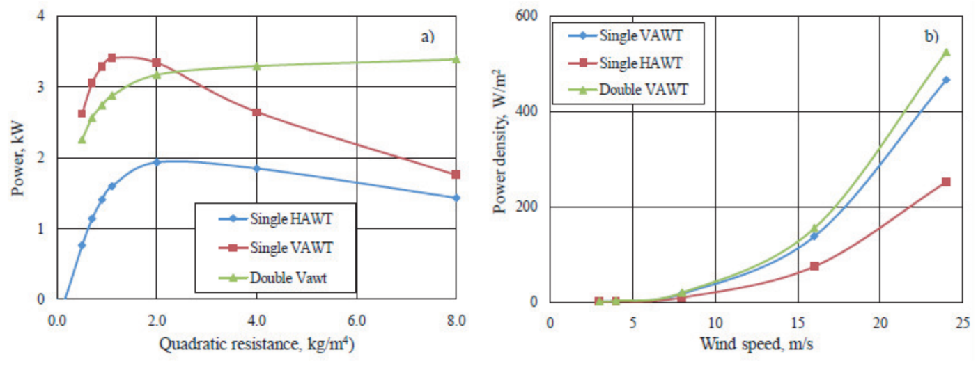
The first simulations run after the independency studies were to investigate the quadratic resistance value which gave the best performance for turbine model. For these simulations, the inlet velocity was kept at 4 m/s, the turbulence was kept to 5%, and the quadratic resistance was varied from 0 to 8 kg/m. For the single large 46 m diameter HAWT, the maximum power generation occurs at 2 kg/m with 1934.5 W generated, after which the power slowly falls off to 1432.2 W at 8 kg/m. For the single VAWT, the power generated climbs from 0 and peaks at 1.1 kg/m, and again after this point, the power tails off. The double VAWT differs in that its maximum power generated is at the highest quadratic resistance level of 8 kg/m after building gently from 0. The values for each step in quadratic resistance are presented in Table 7, Figure 7 and Figure 8.
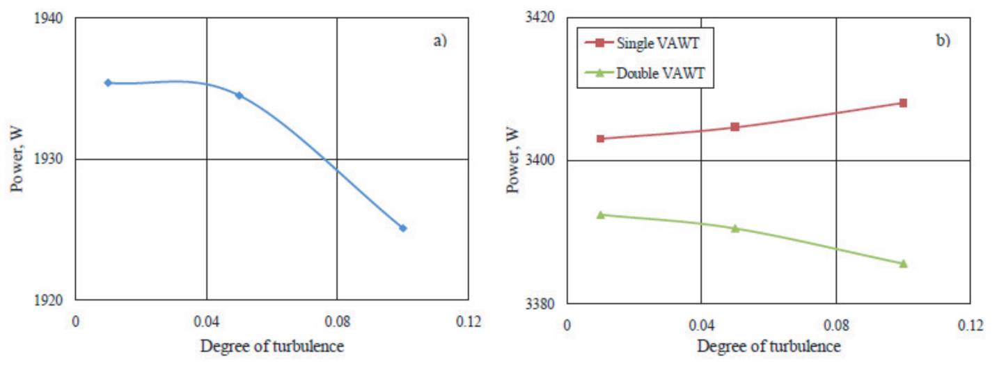
Using the value of quadratic resistance determined previously, each configuration was tested again whilst varying the level of turbulence from 1% to 10%. The inlet speed remained at 4 m/s. The results obtained are shown in Table 8. Out of the three models, the power-generation level of the HAWT turbine did fall more than the VAWTs, as predicted; however, this was only a decrease of 10 W and less than a 1% decrease, whilst the single VAWT power generation varied by 5 W and the double by 7 W. In all cases, the decrease in power generation is not significant.
Wind speed, as shown in Table 9, obviously has the biggest impact on the power produced by the wind turbines as it allows a greater pressure difference to be created. The wind speed was increased from 3 to 24 m/s with the turbulence set to a medium level of 5% and the most suitable quadratic resistance value for each model. The wind speed arriving at the wind turbines is roughly half of that of the wind speed in the predominate wind direction of the north-east due to canalization effect of the valley [6], so to achieve the speeds here the actual wind speed would be roughly doubled, starting at 3 m/s, which is around the cut-in velocity of the average wind turbine. At this level of wind speed, all three turbine models produce a low level of power, with the HAWT producing the least by 43.75%, and both VAWT turbines produce similar levels of power. Throughout the increase in wind speed, the VAWTs track closely with each other, with the HAWT following behind. There is a big step in power from the 4 m/s to 8 m/s, with the VAWTs outperforming the HAWT by 44% again. Further increases to speeds which are unlikely to occur offer a significant power output of almost 740 kW for the single VAWT, again a 44% increase in performance over the HAWT.
However, the power generated does not take into account differences in the area of each turbine, giving an unfair advantage to the larger turbines. The largest turbine is the 46 m diameter HAWT with an area of 1661.9 m, followed closely by the single VAWT with 1584 m. The third model, the double VAWT, has a combined area of 1400 m, and is therefore the smallest. Calculating the power flux density, , takes the area into account and thus allows for a more even comparison. The results are presented in Table 10. Due to its smaller combined area and similar power generation levels, the double VAWT performs best at all wind speeds with around an 11% increase on the single VAWT for all wind speeds. Due to its larger area and lower power output, the single HAWT trails with approximately 48% less power generated per m of area.
When running the simulations to determine the quadratic resistance values for the double VAWT model, there was no definable peak as the power output stayed stable for further increases. As such, it was decided to use 8 kg/m; however, this could signify a problem with the set-up of the simulation and may give a higher power output than is realistic.
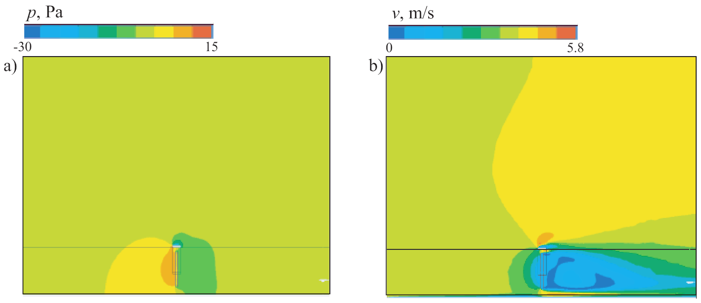
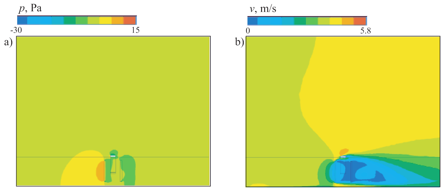
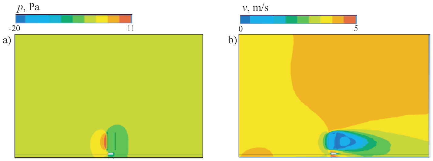
The results of CFD simulations presented in terms of pressure and velocity contours are shown in Figure 9, Figure 10 and Figure 11. The results of numerical simulations show that there was canalization along the combe. The flow faces the actuator disc, modelling the wind turbine blades at a small angle of attack. The wind speed near the porous disc decreases significantly, and flow velocity at the rotor location reaches value, which is 50% of the inlet wind speed. The extracted wind power by the porous disc is substantially affected by the velocity at the rotor location. This means that for the mean wind direction and wind speed in the ravine, the wind under the viaduct is around 3 m/s. This leads to a lower extraction of power from wind as the wind turbine starts to work properly from 6 or 7 m/s. However, the wind flow is conducted through the ravine, arriving at the discs in an almost normal direction. This effect is an interesting point as it can be seen how local wind flow is modified with respect to the prevailing wind in the area in order to face the rotor surfaces. Similar effects were observed in [6]. Adding a VAWT did not affect the mass flow through the rotor surface of the disc.
The upstream flow does not utilize the entire surface of the simulated rotor. This effect occurs for HAWT, and could be produced by the effect of the ground in the wind flow due to the boundary layer. It decelerates the wind near the terrain surface. The power production in the design option with single or double VAWTs is considerably increased as the available extraction surface is also highly increased. In this case, the wind stream occupies the entire surface available, which results in a better exploitation of the available rotor. This effect leads to a higher power flux density (concentration of watts per meter squared) for both variants of VAWTs.
The study into the ability of VAWTs to outperform HAWTs under turbulent conditions was inconclusive, as the results do not show a significant effect. More research and a wider range of data would be required to clarify how turbulence affects both types of turbine. As expected, an increase in wind speeds does provide a significant increase in power; however, the sort of power levels that would be desired are not generated at realistic wind speed levels. From the results, it appears clear that the smaller double VAWTs perform better than the other two; however, this is likely to be mainly due to the superior location above the viaduct which a smaller, lighter turbine could take advantage of. Above the turbine, the wind speed is higher and less turbulent, and is therefore more suited to the extraction of wind energy.
8. Conclusions
As expected, an increase in wind speeds does provide a significant increase in power. From the results, it appears clear that the smaller double VAWTs perform much better than the other two; however, this is likely to be mainly due to the superior location above the viaduct which a smaller lighter turbine could take advantage of. Above the turbine, the wind speed is higher and less turbulent, and therefore more suited to the extraction of wind energy.
An important point to note is that the actual efficiency of the turbines was not taken into account, and this will have a significant effect on the power generated by them and may allow the HAWT to claw back some ground on the VAWTs as they are generally thought of as being less efficient in practice. The location, local wind resources, and siting are important factors in determining the power generated from a wind turbine. A smaller turbine sited in a better location performs better than a larger one that is poorly sited. Smaller turbines also have the advantage of being lighter in both the turbine and its supporting structure, thus reducing the cost and environmental impact.
While this study provided a comparison between various configurations of wind turbines based on the CFD and actuator disc method, it is also important to mention its limitations. The study has been performed with the SST turbulence model. Although advanced turbulence modelling techniques provide high-fidelity results, the computational requirements of the method are high. For further research, the use of artificial canalization could be undertaken, for instance by constructing ducting that will channel a greater amount of air to the turbine and enhance the pressure differential.
Author Contributions
Conceptualization, S.H. and K.V.; methodology, S.H.; software, I.O.; validation, S.H. and I.O.; formal analysis, K.V.; investigation, S.H.; resources, K.V.; writing—original draft preparation, K.V.; writing—review and editing, I.O.; visualization, S.H.; supervision, K.V. All authors have read and agreed to the published version of the manuscript.
Funding
The research is partially funded by Ministry of Science and Higher Education of Russian Federation as part of World-Class Research Centers program “Advanced Digital Technologies” (contract No. 075-15-2020-903 dated 16 November 2020).
Institutional Review Board Statement
Not applicable.
Informed Consent Statement
Not applicable.
Conflicts of Interest
The authors declare no conflict of interest.
References
- El-Shatter, T.F.; Eskandar, M.N.; El-Hagry, M.T. Hybrid PV/fuel cell system design and simulation. Renew. Energy 2002, 27, 479–485. [Google Scholar] [CrossRef]
- Araujo, J.C.H.; de Souza, W.F.; de Andrade Meireles, A.J.; Brannstrom, C. Sustainability challenges of wind power deployment in coastal Ceara State, Brazil. Sustainability 2020, 12, 5562. [Google Scholar] [CrossRef]
- Heath, M.A.; Walshe, J.D.; Watson, S.J. Estimating the potential yield of small building-mounted wind turbines. Wind Energy 2007, 10, 271–287. [Google Scholar] [CrossRef] [Green Version]
- Smith, R.F.; Killa, S. Bahrain World Trade Center (BWTC): The first large-scale integration of wind turbines in a building. Struct. Des. Tall Spec. Build. 2007, 16, 429–439. [Google Scholar] [CrossRef]
- Oppenheim, D.; Owen, C.; White, G. Outside the square: Integrating wind into urban environments. Refocus 2004, 5, 32–35. [Google Scholar] [CrossRef]
- Soto Hernandez, O.; Volkov, K.; Martin Mederos, A.C.; Medina Padron, J.F.; Feijoo Lorenzon, A.E. Power output of a wind turbine in an already existing viaduct. Renew. Sustain. Energy Rev. 2015, 48, 287–299. [Google Scholar] [CrossRef]
- Bhutta, M.M.A.; Hayat, N.; Farooq, A.U.; Ali, Z.; Jamil, S.R.; Hussain, Z. Vertical axis wind turbine: A review of various configurations and design techniques. Renew. Sustain. Energy Rev. 2012, 16, 1926–1939. [Google Scholar] [CrossRef]
- Simisiroglou, N.; Polatidis, H.; Ivanell, S. Wind farm power production assessment: Introduction of a new actuator disc method and comparison with existing models in the context of a case study. Appl. Sci. 2019, 9, 431. [Google Scholar] [CrossRef] [Green Version]
- Lawn, C.J. Optimization of the power output from ducted turbines. J. Power Energy 2003, 217, 107–117. [Google Scholar] [CrossRef]
- Watson, S.J.; Infield, D.G.; Barton, J.P.; Wylie, S.J. Modelling of the performance of a building-mounted ducted wind turbine. J. Phys. Conf. Ser. 2007, 75, 012001. [Google Scholar] [CrossRef]
- Harrison, M.E.; Batten, W.M.J.; Myers, L.E.; Bahaj, A.S. A comparison between CFD simulations and experiments for predicting the far wake of horizontal axis tidal turbines. In Proceedings of the 8th European Wave and Tidal Energy Conference, Uppsala, Sweden, 7–10 September 2009; pp. 566–575. [Google Scholar]
- Bai, L.; Spence, R.R.G.; Dudziak, G. Investigation of the influence of array arrangement and spacing on tidal energy converter (TEC) performance using a 3-dimensional CFD model. In Proceedings of the 8th European Wave and Tidal Energy Conference, Uppsala, Sweden, 7–10 September 2009; pp. 654–660. [Google Scholar]
- Hartwanger, D.; Horvat, A. 3D modelling of a wind turbine using CFD. In Proceedings of the NAFEMS UK Conference, Cheltenham, UK, 10–11 June 2008. [Google Scholar]
- Paraschivoiu, I. Wind Turbine Design with Emphasis on Darrieus Concept; Polytechnic International Press: Montreal, Canada, 2002. [Google Scholar]
- Bulat, P.V.; Volkov, K.N. Simulation of incompressible flows in channels containing fluid and porous regions. Int. J. Ind. Syst. Eng. 2020, 34, 283–300. [Google Scholar]
- Menter, F.R. Two-equation eddy-viscosity turbulence models for engineering applications. AIAA J. 1994, 32, 1598–1605. [Google Scholar] [CrossRef] [Green Version]
- Volkov, K. Multigrid and Preconditioning Techniques in CFD Applications; Springer International Publishing: Berlin/Heidelberg, Germany, 2018; pp. 83–149. [Google Scholar]
- Kozelkov, A.S.; Lashkin, S.V.; Tsibereva, Y.A.; Volkov, K.N.; Tarasova, N.V. An implicit algorithm of solving Navier-Stokes equations to simulate flows in anisotropic porous media. Comput. Fluids 2018, 160, 164–174. [Google Scholar] [CrossRef] [Green Version]
- Weibull, W. A statistical distribution function of wide applicability. J. Appl. Mech. 1951, 18, 293–297. [Google Scholar] [CrossRef]
- Justus, C.G.; Mikhail, A. Height variation of wind speed and wind distribution statistics. Geophys. Res. Lett. 1976, 3, 261–264. [Google Scholar] [CrossRef]
- Bechrakis, D.A.; Sparis, P.D. Simulation of the wind speeds at different heights using artificial neural networks. Wind Eng. 2000, 24, 127–136. [Google Scholar] [CrossRef]
- Ray, M.L.; Rogers, A.L.; McGowan, J.G. Analysis of wind shear models and trends in different terrains. In Proceedings of the American Wind Energy Association Windpower, Anaheim, CA, USA, 22–25 May 2006. [Google Scholar]
Figure 1.
Original domain (a) and new domain (b).

Figure 2.
Different configurations of wind turbines: (a) single HAWT, (b) single VAWT, (c) double VAWT.
Figure 2.
Different configurations of wind turbines: (a) single HAWT, (b) single VAWT, (c) double VAWT.

Figure 3.
Wind rising at 80 m at point (432450, 3109650) taken from IDEA.

Figure 4.
Domain-independent study: (a) average pressure, (b) power output, (c) induced velocity, (d) mass flow rate.
Figure 4.
Domain-independent study: (a) average pressure, (b) power output, (c) induced velocity, (d) mass flow rate.

Figure 5.
Mesh 4 used in CFD calculations for HAWT.

Figure 6.
Mesh-independent study: (a) average pressure, (b) power output, (c) induced velocity, (d) mass flow rate.
Figure 6.
Mesh-independent study: (a) average pressure, (b) power output, (c) induced velocity, (d) mass flow rate.

Figure 7.
Power generated as a function of (a) quadratic resistance, (b) wind speed.

Figure 8.
Power generated by HAWT (a) and VAWT (b) as a function of degree of turbulence.

Figure 9.
Pressure contours (a) and velocity contours (b) for single HAWT.

Figure 10.
Pressure contours (a) and velocity contours (b) for single VAWT.

Figure 11.
Pressure contours (a) and velocity contours (b) for double VAWT.


Table 1.
ITC wind data.
| z, m | 40 | 60 | 80 |
| v, m/s | 6.25 | 6.68 | 6.99 |
| c | 2.271 | 2.285 | 2.276 |
Table 2.
IDAE wind data.
| z, m | 30 | 60 | 80 | 100 |
| v, m/s | 5.57 | 6.34 | 6.69 | 6.91 |
| c | 2.271 | 2.285 | 2.276 | 2.246 |
| C | 6.05 | 6.91 | 7.29 | 7.56 |
Table 3.
Dimensions of computational domain.
| Domain | Height, m | Width, m |
|---|---|---|
| Domain 1 | 100 | 350 |
| Domain 2 | 150 | 450 |
| Domain 3 | 250 | 550 |
| Domain 4 | 300 | 650 |
| Domain 5 | 400 | 850 |
Table 4.
Results of domain independence study.
| Domain | , Pa | % | , Pa | % | , m/s | % | , kg/s | % | P, kW | % |
|---|---|---|---|---|---|---|---|---|---|---|
| Domain 1 | 8.746 | 3.93 | 1.78 | 0.064 | 4.64 | 1652 | 1.59 | 14.09 | 1.48 | |
| Domain 2 | 8.409 | 2.46 | 1.36 | 0.067 | 1.32 | 1626 | 0.56 | 14.30 | 0.14 | |
| Domain 3 | 8.205 | 0.43 | 0.55 | 0.068 | 2.07 | 1617 | 0.12 | 14.32 | 2.12 | |
| Domain 4 | 8.170 | 0.71 | 0.94 | 0.066 | 0.78 | 1615 | 0.12 | 14.11 | 0.64 | |
| Domain 5 | 8.112 | — | — | 0.067 | — | 1617 | — | 14.11 | — |
Table 5.
Number of mesh elements and nodes.
| Mesh | Elements | Nodes | Yplus |
|---|---|---|---|
| Mesh 1 | 1,699,380 | 500,828 | 182 |
| Mesh 2 | 1,706,173 | 505,195 | 171 |
| Mesh 3 | 1,829,597 | 546,562 | 156 |
| Mesh 4 | 2,041,625 | 606,166 | 124 |
| Mesh 5 | 2,960,299 | 885,269 | 86 |
| Mesh 6 | 3,895,222 | 1,186,877 | 52 |
Table 6.
Results of mesh independence study.
| Mesh | , Pa | % | , Pa | % | , m/s | % | , kg/s | % | P, kW | % |
|---|---|---|---|---|---|---|---|---|---|---|
| Mesh 1 | 8.383 | 0.32 | 0.71 | 0.065 | 0.62 | 1631 | 0.06 | 13.86 | 0.58 | |
| Mesh 2 | 8.410 | 0.01 | 1.11 | 0.064 | 4.13 | 1630 | 0.25 | 13.78 | 3.70 | |
| Mesh 3 | 8.409 | 0.68 | 0.72 | 0.067 | 1.66 | 1626 | 0.12 | 14.30 | 1.91 | |
| Mesh 4 | 8.424 | 0.40 | 0.58 | 0.066 | 9.96 | 1624 | 0.31 | 14.03 | 9.96 | |
| Mesh 5 | 8.390 | 0.27 | 0.47 | 0.073 | 9.71 | 1629 | 0.12 | 15.50 | 10.17 | |
| Mesh 6 | 8.367 | — | — | 0.080 | — | 1631 | — | 17.16 | — |
Table 7.
Power generated (in W) at each quadratic resistance value.
| K, kg/m | Single HAWT | Single VAWT | Double VAWT |
|---|---|---|---|
| 8.0 | 1432.20 | 1757.3 | 3390.5 |
| 4.0 | 1847.40 | 2646.9 | 3291.2 |
| 2.0 | 1934.50 | 3338.3 | 3170.4 |
| 1.1 | 1599.00 | 3404.6 | 2877.8 |
| 0.9 | 1408.30 | 3287.8 | 2742 |
| 0.7 | 1137.00 | 3054.3 | 2562.8 |
| 0.5 | 761.60 | 2621.9 | 2256.8 |
| 0.1 | 552.45 | 856.86 | |
| 0.0 | 17.379 |
Table 8.
Effect of turbulence level on power output (in W).
| Turbulence | Single HAWT | Single VAWT | Double VAWT |
|---|---|---|---|
| 10% | 1925.10 | 3408.0 | 3385.6 |
| 5% | 1934.50 | 3404.6 | 3390.5 |
| 1% | 1935.40 | 3403.0 | 3392.4 |
Table 9.
Power generated (in W) at varying wind speeds.
| Wind Speed, m/s | Single HAWT | Single VAWT | Double VAWT |
|---|---|---|---|
| 3 | 0.81 | 1.44 | 1.43 |
| 4 | 1.93 | 3.41 | 3.40 |
| 8 | 15.45 | 27.25 | 27.14 |
| 16 | 123.94 | 218.37 | 217.32 |
| 24 | 419.29 | 739.07 | 735.18 |
Table 10.
Power flux density (in W/m).
| Wind Speed, m/s | Single HAWT | Single VAWT | Double VAWT |
|---|---|---|---|
| 3 | 0.49 | 0.91 | 1.02 |
| 4 | 1.16 | 2.15 | 2.43 |
| 8 | 9.30 | 17.21 | 19.38 |
| 16 | 74.58 | 137.86 | 155.23 |
| 24 | 252.30 | 466.58 | 525.13 |
Publisher’s Note: MDPI stays neutral with regard to jurisdictional claims in published maps and institutional affiliations. |
© 2021 by the authors. Licensee MDPI, Basel, Switzerland. This article is an open access article distributed under the terms and conditions of the Creative Commons Attribution (CC BY) license (https://creativecommons.org/licenses/by/4.0/).
Share and Cite
MDPI and ACS Style
Handsaker, S.; Ogbonna, I.; Volkov, K. CFD Prediction of Performance of Wind Turbines Integrated in the Existing Civil Infrastructure. Sustainability 2021, 13, 8514. https://doi.org/10.3390/su13158514
AMA Style
Handsaker S, Ogbonna I, Volkov K. CFD Prediction of Performance of Wind Turbines Integrated in the Existing Civil Infrastructure. Sustainability. 2021; 13(15):8514. https://doi.org/10.3390/su13158514
Chicago/Turabian StyleHandsaker, Samuel, Iheanyichukwu Ogbonna, and Konstantin Volkov. 2021. "CFD Prediction of Performance of Wind Turbines Integrated in the Existing Civil Infrastructure" Sustainability 13, no. 15: 8514. https://doi.org/10.3390/su13158514
Note that from the first issue of 2016, this journal uses article numbers instead of page numbers. See further details here.