
Abstract
Urban rail transit connecting with a comprehensive transportation hub should meet passenger demands not only within the urban area, but also from outer areas through high-speed railways or planes, which leads to different characteristics of passenger demands. This paper discusses two strategies to deal with these complex passenger demands from two aspects: transit train formation and real-time holding control. First, we establish a model to optimize the multi-marshalling problem by minimizing the trains’ vacant capacities to cope with the fluctuation of demand in different periods. Then, we establish another model to control the multi-marshalling trains in real time to minimize the passengers’ total waiting time. A genetic algorithm (GA) is designed to solve the integrated two-step model of optimizing the number, timetable and real-time holding control of the multi-marshalling trains. The numerical results show that the combined two-step model of multi-marshalling operation and holding control at stations can better deal with the demand fluctuation of urban rail transit connecting with the comprehensive transportation hub. This method can efficiently reduce the number of passengers detained at the hub station as well as the waiting time without increasing the passengers’ on-train time even with highly fluctuating passenger flow.
1 Introduction
A comprehensive transportation hub connecting with multiple transportation modes is the key to connecting and transferring traffic from inside and outside a metropolis. Urban rail transit has been built and is operated in many cities due to its advantages of large capacity, high efficiency, and punctuality. Its stable operation connecting to the hub not only directly promotes the operation of various traffic modes, but also benefits the effective integration of urban internal and external traffic.
For an urban rail transit line connected with hubs, passenger demand comes not only from the daily commuter passengers within the city but also from the outer transportation modes connected with the comprehensive transportation hub. Daily commuter passenger demand inside the city has an obvious tidal phenomenon and clearly fluctuates throughout the day; the arriving passenger demand from outer transportation modes connected with the hub presents intermittent short-term high-intensity characteristics. In addition, outer transportation modes connected with the hub are often delayed due to weather or other factors, resulting in randomness of passenger arrival time.
The current strategy of many rail transit companies is adjusting the train departure time or headway during different time intervals of the day to match the transportation capacity supply with the fluctuating daily commuter passenger demand; that is, there is a small interval for peak demand and a large interval for off-peak demand. This causes a much different waiting time for passengers arriving at the station at different time, especially during the period between the peak hours and the off-peak hours [1]. With the arriving passenger demand from outer transportation, this strategy makes it hard to deal with the complex passenger demands and to balance the waiting time of different passengers throughout the day. In addition, when outer transportation modes arrive at random because of delay, it is likely to cause an increase in waiting time for some passengers.
The fluctuation in passenger demand at different periods greatly affects the operational efficiency of public transportation. In recent years, many studies have been conducted on public carriage operation control and multi-carriage operation organization to reduce the effect of passenger demand fluctuation and improve the service level of public transportation.
-
(1)
Station control
With the development of science and technology, the real-time state information of the system is taken into consideration in the process of carriage operation control. Zhao et al. [2] proposed a distributed control scheme to minimize the sum of waiting time at station and in-carriage time. Yu and Yang [3] proposed a two-step operation control strategy to minimize the sum of passenger waiting time and on-board time, while Grube and Cipriano [4] proposed two real-time stop control strategies for subway lines to minimize passengers’ waiting time. Sánchez-Martinez et al. [5] considered the dynamic passenger arrival rate and running time between stations and optimized carriage station control time in order to minimize the waiting time during the period. Wu et al. [6] considered the delays caused by various types of interference and the real-time arrival information of the carriages at the transfer station, and optimized the carriage's extended time at the station with the goal of minimizing the combined cost of passenger waiting time and carriage operating expenses.
Some studies have focused on the combined station control of more than one carriage. For example, Daganzo [7] discussed the control of a pair of vehicles: stopping the following carriage at the station when the headway is reduced and accelerating the following carriage when the headway is increased. Bellei and Gkoumas [8] analyzed the control effects of two-carriage station control strategies on a bus line considering both the dynamic passenger arrival rate and running time between stations. Bartholdi and Eisenstein [9] adjusted the station control duration of the carriage based on the departure interval between the current carriage and the following carriage to achieve balanced departure intervals, while Newell [10] minimized the average waiting time of passengers by performing station control of a pair of vehicles on a route.
Some studies combined carriage station control with other control strategies. Delgado et al. [11] combined carriage station control and passenger number on-board control under the constraint of carriage capacity, and established a quadratic programming model to minimize the total travel time. Subsequently, Delgado and his colleagues [12] compared the results of various control strategies under different combinations of arrival rate and running time between stations using simulation to verify the application conditions and control effect of the combined control strategy. Su and Wilson [13] created a mixed integer programming model to determine whether combined station control and regional carriage operation should be carried out.
-
(2)
Urban rail transit marshalling
Various studies have been conducted on the optimization of urban rail transit marshalling. Based on the passenger flow of urban rail transit, a feasible train operation plan is optimized by integrating various influencing factors. Li et al. [14] studied the routing problem of multi-route and single marshalling trains on Y-type lines. They proposed an integer programming model with the goal of minimizing operating costs and passenger costs. Ding et al. [15] considered the peak-hour line load and proposed a non-linear programming model for the single marshalling of large and small junctions. Fioole et al. [16] presented a model which is an extension of an existing rolling stock model for routing train units along a number of connected train lines. The extended model can also handle combining and splitting of underway trains. Li et al. [17] proposed an optimization model and solution method for the design problem of multi-junction and multi-marshalling train routing with the goal of minimizing the cost of operating companies and the cost of passenger waiting time, considering the passengers' selection behaviors of different trains.
Other scholars have conducted feasibility studies on multiple marshalling schemes for urban rail transit. Niu and Zhang [18] took the intercity railway into consideration and took the overall travel time of passengers as the minimal objective to establish an optimization model for the operation plan of multi-marshalling intercity railway. Du and Guo [19] established a train marshalling optimization model to minimize operating costs and passenger transit costs. The results showed that compared with fixed marshalling schemes, multiple marshalling schemes can reduce enterprise operating costs and passenger transit costs.
In this paper, we focus on the optimal strategy to satisfy the passenger demand not only within the urban area, but also from outer transportation with different characteristics at the comprehensive transportation hub. As shown in Fig. 1, these two types of passengers arriving at the rail station can board on the \(kth\) train if there is no delay of the outer transportation, but they have to take the \(k + 1th\) train if they arrive at the platform after the \(kth\) train leaves the station; moreover, they may have to wait for the \(k + 2th\) train if the \(k + 1th\) train is overly congested.
Fig. 1 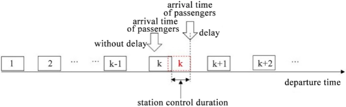
Operation control of rail train
To satisfy passenger demand from both daily commuter and outer transportation, this paper proposes a two-step strategy: (1) adjust the train formation to deal with the short-term high-intensity demand instead of adjusting the train departure interval so as to retain a relatively even headway and a relatively equal average waiting time for all arriving passengers at any time. (2) Control the holding times of the multi-marshalling trains to deal with the random fluctuation in passenger demand. The holding time of trains in this paper considers not only extending the time duration of passengers getting on and off the train, but also those leaving ahead of time, that is, optimizing the dwelling time of the train at the station to take away the greatest number of passengers when the passengers’ arrival time is within the preset time range. As shown in Fig. 1 above, a reasonable dwelling time should be given to the kth train when the passengers’ delay is within the assumed time range so that the delayed passengers can catch up to the kth train without any extra waiting time.

The main contributions of this paper include the following:
-
(1)
A two-step model is proposed to formulate the organization problem of rail transit connecting with a comprehensive transportation hub when the passenger demand is from both an inner urban area and outer transportation.
-
(2)
The model carries out real-time station control for multi-marshalling trains, considering the fluctuation in passenger flow demand caused by the arrival delay of other transportation modes in the junction, and optimizes the trains’ dwelling time control at each station, where dwelling time can be both shorter and longer than the scheduled time.
-
(3)
The model considers not only the fluctuation in passenger demand caused by the scheduled arrival of outer transportation, but also the random fluctuation in passenger demand caused by fluctuating delay in the outer transportation to the hub due to different factors.
The remainder of this paper is organized as follows. In Sect. 2, we formulate the two-step model of rail train organization. Then, a genetic algorithm (GA) solving method is proposed in Sect. 3, and numerical examples are discussed in Sect. 4 to illustrate the properties of the proposed model and the performance of the algorithm. Finally, a summary and conclusions are presented in Sect. 5.
2 Model Formulation
The optimization model proposed in this paper is completed in two steps. In the first step, according to the passenger arrival rate from outer transportation to the transportation hub and the time-varying origin destination (OD) demand between stations along the urban rail transit lines, the model adjusts the trains’ departure time and the corresponding train formations under the constraint that passengers will not wait for more than two trains. The objective is to minimize the spare capacity on the trains when the trains leave the stations during the period, and obtain the optimal multi-marshalling operating scheme and optimal running schedule of the rail transit trains. In the second step, station control of the running trains is optimized to minimize the total waiting time of the passengers on the line during the period as the trains run according to the optimal schedule calculated in the first step, considering the fluctuating arrival of the outer transportation to the hub due to different factors.
In this model, it is assumed that there are N stations in total in the urban rail transit line considered by the model, and K trains are sent out during the study period. Each train departs from station 1 to station N and stops at each station. The symbols used in this article are listed in Table 1.
2.1 Model Assumptions
This paper studies one running direction of an urban rail transit line connecting with a comprehensive transportation hub. Historical passenger flow of each origin destination (OD) along urban rail transit lines can be obtained using the auto fare collection (AFC) data, and arrival schedules of outer transportation at the hub can also be obtained from the transportation hub. In addition, the establishment of the model also requires the following three assumptions:
-
(a)
The running time between any two successive stations is fixed and determined by distance.
-
(b)
Trains of different marshalling groups have the same running properties (speed, acceleration, etc.), and each carriage has the same capacity.
-
(c)
Considering the train capacity (carriage capacity * number of carriages), passengers follow the “first come, first served” principle when waiting at the station, and passengers wait for no more than two trains.
2.2 The First-Step Model
During the study period, the objective is the minimal sum of spare capacity when all trains leave all stations, which is calculated as follows:
where \(c_{{{\text{k}},{\text{i}}}}\) represents the spare capacity of the \(kth\) train when it leaves station i.
In the first step, the constraints include
Equation (2) indicates that each train corresponds to only one of the train types; Eqs. (3) and (4) limit the departure times of the first and last train in the study period; Eq. (5) gives the calculation method of departure interval, which is the difference between the departure time of two adjacent trains at the same station \(i\); Eq. (6) shows that any departure time interval should be within the minimal and maximal departure interval; Eq. (7) represents the recursive relation of departure time during train operation. The departure time of the kth train at station i+1 is equal to the sum of the departure time of the kth train at station i, the running time from station i to station i+1 and the stopping time of the kth train at station i+1. Equation (8) refers to the number of passengers arriving at station \(j\) from station \(i\) when the kth carriage leaves station \(i\); Eq. (9) represents the number of waiting passengers when the kth train leaves station \(i\). Equation (10) shows the actual number of passengers on the kth train when it leaves station \(i\); Eq. (11) is the number of passengers left behind due to the insufficient capacity.
In the model, it is assumed that the arriving passengers follow the first-come-first-served principle, so when the kth train leaves station i, passengers from station j with different destinations have the same probability of getting on the kth train, which is \(\overline{{\beta }_{k,j}}/{\beta }_{k,j}\). Equation (12) represents the number of passengers from station j who can take the kth train when it leaves station i; Eq. (13) shows the number of passengers getting off the kth train when it arrives at station i; Eq. (14) is the number of passengers on board the kth train when it leaves station i; Eq. (15) is the spare capacity of the kth train when it leaves station i; Eq. (16) guarantees that the actual number of passengers in the second train is not less than the number of passengers dropped in the previous train and restricts passengers to wait for at most two trains.
2.3 The Second-Step Model
Suppose that passengers wait for no more than two trains, so their waiting time can be divided into two parts: the necessary waiting time for the first train and the possible waiting time for the second one. During the study period, the objective is the minimal total waiting time of passengers at all stations on the line, which is calculated as follows:
where \(T_{1}\) is the total waiting time for the first train, which is equal to the difference between the time that passengers arrive and the time when their first waiting train leaves the station:
where \(\lambda_{{{\text{i}},{\text{j}}}} \left( t \right)\) is the dynamic passenger arrival rate from station i to destination j, and we set \(td_{0,i} = t_{s}\). \(T_{2} { }\) is extra waiting time for the second train due to the capacity constraint of their first waiting train. The value is the difference between the departure time of the next train and the current train:
In the second step, the station control of trains is optimized based on the multi-marshalling train operation schedule obtained in the first step. The constraints in this step include
Equation (20) is the departure time of the train after station control, and Eq. (21) is the feasible duration of station control. Equation (22) indicates the delay situation. During the study period, the outer mode of transportation arriving at the hub is numbered according to the order of arrival time shown in the timetable. Equation (22) indicates that the number of delayed passengers choosing railway is a when the nth train is delayed for w min. n is randomly selected from the total number of trains arriving during the study period, t represents the delayed time randomly, a is given based on actual data. In the original OD demand matrix, a is subtracted during the normal arrival period of the nth train, and a is added in the period after the delay of w min, and the passenger arrival OD matrix is updated in the case of delay.
3 Solution Algorithm
The number of routes and stations in the model and the number of trains issued during the study period determine the scale of the problem. For urban rail transit lines with generally short carriage intervals, as the study period increases, the number of trains issued during the period also increases considerably. The solution scale of the model will grow rapidly; more importantly, there are various complicated relationships between the parameters involved in the model, and the process of solving the model often requires various parameter values to call each other, so it is difficult to use general analysis to find the optimal solution. The genetic algorithm performs calculations by encoding the decision variables of the problem into the chromosomes processed by the algorithm. Therefore, the encoded decision variables can be used to express the relationship between the parameters, and the mutual calls between the parameters in the solution process can be realized so as to iteratively find the optimal solution to the model. Therefore, in this paper, we chose to solve the optimized model based on a genetic algorithm.
Two genetic algorithms (GA) are adopted in combination to solve the two-step model in this paper. The algorithm steps are as follows:
-
Step 0 Parameter initialization: the number of iterations gen = 0; the initial population size M; the algorithm termination algebra N.
-
Step 1 Perform chromosome coding and repeat it M times to get the initial population.
The gene sequence of the chromosome in Step 1 consists of three parts. K can be repeatedly and randomly selected from V integers representing the group type as the first part of the chromosome; K real numbers that satisfy the constraints (3)-(6) are randomly generated as the second part of the chromosome. The \(K*(N-2)\) randomly generated real numbers satisfying constraints (5)–(7) are taken as the third part of the chromosome.
-
Step 2 Calculate the individual fitness value: \({fitness}_{1}=1/{Z}_{1}\), which is the reciprocal of the objective function in Step 1.
-
Step 3 Determine the number of iterations: If gen = N, output the optimal solution and go to Step 5; otherwise, go to Step 4.
-
Step 4 Perform selection, crossover, and mutation operations in order to obtain the offspring population. Set gen = gen + 1 and go to Step 2.
Selection The selection process in this algorithm uses the roulette method and performs the crossover and mutation operation according to the crossover and mutation probability.
Crossover: First, randomly select two chromosomes from M chromosomes, then randomly select a gene position within the length of the gene sequence, and directly exchange the genes for the same position. To complete the crossover operation, it is necessary to ensure that the second part satisfies constraints (3)–(6), and the third part satisfies constraints (5)–(7). Repeat the above process M/2 times until all individuals in the population are traversed.
Mutation First select an arbitrary chromosome and randomly select a gene position to mutate. If the gene position is within the range of the first part, randomly select a gene from the V integers to replace the current position; if the gene position is in the second or third range, the number of genes at that position is randomly increased or decreased by a suitable value. To complete the mutation operation, it is necessary to ensure that the second part satisfies constraints (3)–(6), and the third part satisfies constraints (5)–(7); otherwise, it must be mutated again until the constraints are satisfied. Repeat M times until all individuals in the population are traversed.
-
Step 5 Using the optimal solution obtained in Step 3 to execute the second GA.
-
Determine the population size M and the maximal evolution algebra N suitable for the second genetic algorithm, and initialize the iteration count gen=0. Use real numbers to encode the chromosome, and the randomly generated \(K*\left(N-2\right)\) real numbers satisfying Eq. (21) are treated as chromosomes.
-
Step 6 Calculate the objective value and set the fitness function as \({fitness}_{2}=1/{Z}_{2}\).
-
Step 7 Determine the number of iterations: if gen = N, output the optimal solution and stop; otherwise, perform selection, crossover, and mutation operations to obtain the offspring population. Set gen = gen + 1 and go to Step 6.
4 Case Analysis
Beijing West Railway Station is a comprehensive transportation hub located in the west of Beijing, with a yard scale of 10 platforms. The Beijing West Railway Station is not only a transfer station between Beijing Metro Line 9 and Line 7, but also a big railway station in Beijing, and the passengers taking on and off this station include those from central city and outer suburban areas. The network of the metro lines and railway lines crossing Beijing West Railway Station is shown in Fig. 2. As Beijing Metro Line 9 has a comprehensive transportation hub (Beijing West Railway Station), it was taken as the case study in this paper. Beijing Metro Line 9 is a longitudinal trunk line in the west of Beijing. The total length of the line is 16.5km with north-south trend. There are 13 stations, including 7 transfer stations. It transfers with Line 4 at National Library in the north and transfers with Fangshan Line at Guogongzhuang in the south. Each train of Beijing Metro Line 9 has 6 uniform B-type carriages and a marshalling capacity of 1440 passengers. The maximal speed of the train is designed to 80 km/h. Trains are operated in different frequencies during the day. In morning and evening peak hours on weekdays, the headway is 4 min, and 6 min in off-peak hours. The dwelling time of train at each stop is 30–45 s. Passenger restriction measure is adopted at Beijing West Railway Station throughout the day, that is, the number of passengers entering the platform is controlled according to the congestion state.

Network of the metro lines and railway lines crossing Beijing West Railway Station
During the period [7:30 am, 9:10 am], which is the morning peak hour, collecting the passenger data from AFC every 5 min and the arrival of outer transportation at the hub, we obtain the passenger demand distribution of Beijing Metro Line 9 at the hub as shown in Fig. 3.

Passenger demand at the hub (Beijing West Railway Station) of Beijing Metro Line 9
It can be seen from Fig. 3 that without current restrict measure, the demand fluctuates significantly for every 5 min and the overall trend is downward.
4.1 Parameter Setting
Two types of train marshalling: 4-car marshalling of 960 passengers capacity and 8-car marshalling of 1920 passengers capacity on the Beijing Metro Line 9 were considered. The direction from National Library to Guogongzhuang Station is considered and the headway is between 4.85 and 5.15 min. It is assumed that the train runs at a constant speed without interference during the operation between stations, regardless of the acceleration and deceleration of the train entering and leaving the station, the running time between stations is the ratio of the distance between the stations to the running speed, and the same value is used for trains in different formations. The running time data between stations along this line are given in Table 2. The dwelling times of different trains at each station are between 30 s and 45 s.
The random fluctuation in demand caused by the delay of outer transportation is represented by a random function. The outer transportation arriving at Beijing West Railway Station during the study period [7:30 am, 9:10 am] is numbered according to the scheduled arrival time, and then a random function \(\xi (x,t)\) is used to indicate the delay situation.
4.2 Other Operating Strategies
We denote the two-step train operation strategy in this paper as full strategy (FS) and three comparative train operation strategies are defined: strategy 1 (S1), strategy 2 (S2) and strategy 3 (S3) as shown in Table 3. These three operation strategies can be achieved by adjusting the optimization model in this paper.
-
S1
The train marshalling is fixed to 6 and the first step is omitted. The scheduled headway of 1-9 trains is fixed to 4 min, and that of 10-18 trains is fixed to 6 min. S1 is the current train operation strategy in use when the arrival of the outer transportation at the hub fluctuates.
-
S2
The train marshalling is fixed of 6 and the first step is omitted. The scheduled headway of 1-9 trains is fixed to 4 min, and that of 10-18 trains is fixed 6 min. The second step of station control is the same as that of FS.
-
S3
It has only the first step of marshalling optimization process, and the second step is omitted.
In addition, the second step of the above four strategies is based on the consideration of the delay in the arrival of the Beijing West Railway Station. In order to compare the situation when no delay occurs, the S1 and FS are applied to the situation with no delay and are denoted as S1-N and FS-N, respectively.
Other parameters in the GA include: \(M=50\), \(N=500\), \({P}_{c}=0.8\), and \({P}_{m}=0.5\). The above six cases are solved and the numerical results are analyzed in the following section.
4.3 Numerical Results
During the study period [7:30 am, 9:10 am], regardless of the unstable operation results of the first 20 min, the calculation results of the six cases during time period [7:50 am, 9:10 am] are mainly focused on the matching of train supply and passenger demand, the passenger waiting time, the train travel time, and the number of people left behind at the station.
-
(1)
Matching of train supply and passenger demand
First, the matching of train supply with passenger demand is measured by the difference between the passenger demand and the number of passengers getting on the rail transit line in each unit period: the smaller the difference, the higher the degree of matching. In the period of [7:50 am, 9:10 am], passenger demand and the number of passengers boarding on the line at the hub under different strategies are both counted every 5 min and are drawn in Figs. 4 and 5 showing the difference.
Fig. 4 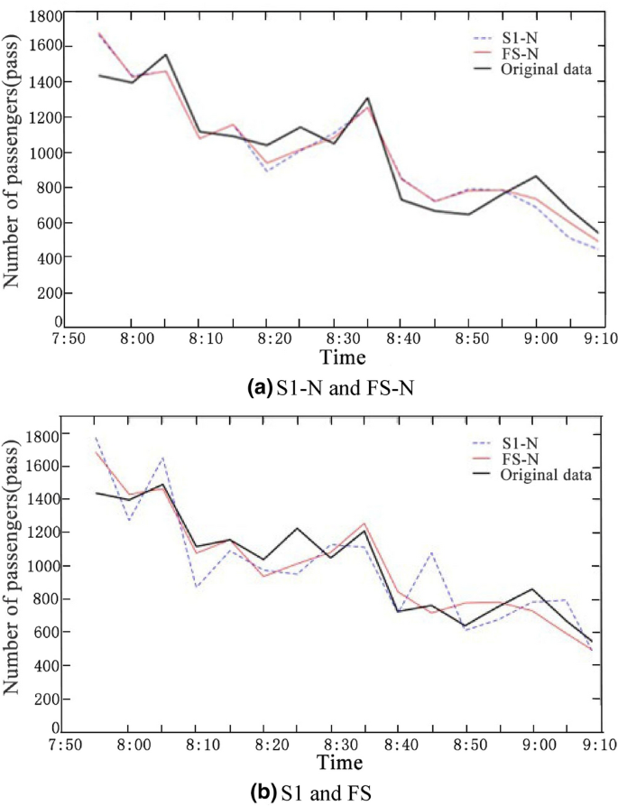
Passenger demand and train supply
Fig. 5 
Number of passengers stranded
Figure 4(a) shows that if the outer transportation is operated strictly according to the schedule and has no fluctuation, peak and off-peak strategy (S1-N) can work almost as well as FS-N to supply the passenger demand at the hub, even though FS-N is slightly better. But if the arrival time of outer transportation is not on schedule, FS shows much better ability to deal with the fluctuation in passenger demand as shown in Fig. 4(b). In fact, the delay of outer transportation indeed exists. If the delay information is released a relatively long beforehand, the train marshalling can be optimized to deal with this situation; if the delay information is obtained in real time, the station control of the train is very effective.
-
(2)
Passengers left behind
In this example, the numbers of passengers left behind after each train leaves each station are compared between four cases: S1-N, FS-N, S1 and FS, and the results are shown in Fig. 5. Among them, the meanings of scale values and units of the coordinate axes in each graph are the same, the x-axis represents the train number, the y-axis represents the station number on the line except the last station, and the z-axis represents the number of stranded passengers.
On the whole, in the direction of the station, the peak number of passengers staying in the station mainly appears on the Beijing West Railway Station and its nearby stations; in the direction of the train number, the peak number of passengers staying in the station mainly appears in the lower number of trains. The reasons for the results of the four cases are different. For the cases of formation optimization and site control (FS and FS-N), it is because the proportion of small formations is large in the following trains. For the cases without formation optimization and site control (S1-N and S1), it is because the rear train departure interval is large.
From the comparison of Fig. 5(c) and d, it can be seen that the number of passengers stranded at the stations is significantly reduced after the optimization of the marshalling and site control in the case of considering the arrival delay of the outer transportation. The same conclusion can also be obtained without considering the delay of the arrival of the outer transportation (Fig. 5a and b). On the other hand, by comparing Fig. 5(a) and c or b and d, we find that there are a few more passengers staying at the site when there is a delay than when there is no delay.
Through the above analysis, it can be found that regardless of whether the delay of the outer transportation arrival of the outer transportation is considered, the optimization of train formation and station control can effectively reduce the number of people stranded at stations and quickly dissipate the arrival of passengers at the junction.
-
(3)
Average passenger waiting time
During the period of [7:50 am, 9:10 am], the average waiting time per passenger was calculated every 5 min for the six cases and the results are shown in Table 4. The third column in the table represents the degree of improvement relative to the peak-and-off-peak departure interval strategy (corresponding S2-N or S2), and the fourth column represents the standard deviation of the average waiting time.
Table 4 Average waiting time According to the results in Table 4, all strategies have improvement in average waiting time per passenger compared to the strategy of only peak-and-off-peak departure interval with and without outer transportation delay. If the outer transportation can arrive strictly according to the schedule and the passenger demand is fixed, the average waiting time of FS-N has a reduction of 5.47% and a better stability (smaller standard deviation) compared to that of S1-N. If the outer transportation cannot arrive on time and have more or less delay, FS has even more advantage to reduce the average waiting time (a reduction of 8.17%) and to level off the standard deviation (from 1.08 to 0.84). S2 and S3 are better than S1 but worse than FS from these two respects. In sum, FS can do better both in reducing the total waiting time (same as average waiting time) and in averaging the waiting time to each passenger.
-
(4)
Total travel time of the train
The total travel times of the entire trips for 18 trains in four strategies with and without outer transportation delay are compared. Because the station control of all the trains is from the point of passengers, some trains have shorter total travel time compared to scheduled travel time, while other trains have longer total travel time. But the total travel time is concentrated at about 27.5 minutes, and the fluctuation among all trains is not apparent. The average travel time and standard deviation of each train for the four cases are shown in Table 5. From Table 5 we also find that if the outer transportation arrives on time, the strategy FS can even reduce the average travel time of the trains; on the other hand, if the outer transportation does not arrive on time, the average travel time of the trains has only increased 0.025 min, which means that FS has a small change in travel time (also the on-board time of passengers) and obtains a large reduction in the passengers’ waiting time.
Table 5 Average travel time and standard deviation -
(5)
Feasibility analysis
According to the optimal results of the train marshalling in this paper, the 2nd, 3rd, 4th, 5th, 6th, 8th, and 11th trains adopt the 8-car marshalling, and the remaining trains use the 4-car marshalling. The 18 trains in the study period require a total of 100 cars. A total of 45,432 passengers are transported. The S2 that does not consider train marshalling optimization adopted a single 6-car marshalling. The 18 trains in the study period require a total of 108 cars, and a total of 46,063 passengers were transported. It can be found that the optimized model of this paper only reduces the passenger flow by 1.37% but saves 8 cars during the study period with little change in the travel time of the trains. Therefore, from the point of operating costs, the multi-marshalling scheme can be adopted.
When the outer transportation mode does not arrive at Beijing West Railway Station according to the schedule, the delayed passenger arrival data is updated and the real-time control of the transit train is optimized. The algorithm optimization time is about 60 s, which is much shorter than the time interval between passengers arriving at Beijing West Railway Station and transferring to Beijing Metro Line 9, so that the train can update the stop time of the train according to the optimized control time. Therefore, the real-time station control of transit trains can be realized.


5 Conclusions
This paper analyzes the characteristics of passenger demand of urban rail transit lines connecting to integrated transportation hubs and establishes a combined two-step model of train formation optimization and real-time station control. The two-step model is solved successively by two GAs.
The main conclusions of this paper are as follows: the numerical results show that regardless of whether the outer transportation arrives on time or not, after the train marshalling optimization and real-time station control, the train supply capacity and the passenger demand are more equally matched, the number of waiting passengers per train is reduced, and the waiting time of passengers arriving at different periods is more balanced. Moreover, the model can reduce passenger waiting time without increasing passengers’ on-board time; at the same time, the current passenger flow-limiting measures are unnecessary, which increases the waiting time of passengers and leaves a large number of passengers stranded in the hub station.
On the basis of the research in this paper, we can consider further discussions in the following aspects:
-
(1)
When the delay of the outer transportation is too long, and the passenger demand changes excessively, it should be reflected in the first step of train marshalling optimization.
-
(2)
It is necessary to consider real-time updating of all kinds of information that affects the passenger demand and to utilize it in station control of trains in real time and even train marshalling optimization.
References
Guo X, Sun H, Wu J (2017) Multiperiod-based timetable optimization for metro transit networks. Transp Res Part B: Methodol 96:46–67
Zhao J, Bukkapatnam S, Dessouky MM (2005) Distributed architecture for real-time coordination of bus holding in transit networks. Intell Transp Syst IEEE Trans 4(1):43–51
Yu B, Yang Z (2009) A dynamic holding strategy in public transit systems with real-time information. Appl Intell 31(1):69–80
Grube P, Cipriano A (2010) Comparison of simple and model predictive control strategies for the holding problem in a metro train system. J Transp Res Board 2343(1):17–24
Sánchez-Martinez GE, Koutsopoulos HN, Wilson NHM (2016) Real-time holding control for high-frequency transit with dynamics. Transp Res Part B 83:1–19
Wu W, Liu R, Jin W (2016) Designing robust schedule coordination scheme for transit networks with safety control margins. Transp Res Part B 93:495–519
Daganzo CF (2009) A headway-based approach to eliminate bus bunching: Systematic analysis and comparisons. Transp Res Part B: Methodol 43(10):913–921
Bellei G, Gkoumas K (2009) Threshold - and information-based holding at multiple stops. IET Intel Transport Syst 3(3):304–313
Bartholdi JJ, Eisenstein DD (2012) A self-coordinating bus route to resist bus bunching. Transp Res Part B 46(4):481–491
Newell GF (2016) Control of pairing of vehicles on a public transportation route, two vehicles, one control point. Transp Sci 8(3):248–264
Delgado F, Munoz JC, Giesen R (2009) Real-time control of buses in a transit corridor based on vehicle holding and boarding limits. Transp Res Record J Transp Res Board 2090(2090):59–67
Delgado F, Munoz JC, Giesen R (2012) How much can holding and/or limiting boarding improve transit performance. Trans Res Part B Methodol 46(9):1202–1217
Su S, Wilson NHM (2001) An optimal integrated real-time disruption control model for rail transit systems. Computer Aided Scheduling of Public Transport 335-363.
Li DW, Liu ZJ, Wang XQ et al (2018) Routing plan for y-type line of Urban rail transit considering passenger choice behavior. China Railway Sci 39(4):114–122
Ding XQ, Guan ST, Sun DJ et al (2018) Short turning pattern for relieving metro congestion during peak hours: the substance coherence of Shanghai China. Eur Transp Res Rev 10(2):1–11
Fioole PJ et al (2005) A rolling stock circulation model for combining and splitting of passenger trains. Eur J Oper Res 174(2):1281–1297
Li ZY, Zhao J, Peng QY (2020) Optimizing the train service route plan in an Urban rail transit line with multiple service routes and multiple train sizes. J China Railway Soc 42(06):1–11
Niu H, Zhang M (2012) An Optimization to schedule train operations with phase-regular framework for intercity rail lines. Discrete Dynamic in Nature and Society: 348-349.
Du XT, Guo JL (2019) Research on grouping optimization of Urban rail transit trains. Softw Guide 18(5):146–150
Acknowledgements
This work is jointly supported by the National Natural Science Foundation of China (71621001, 71771019, 72091513, and 71871130).
Author information
Authors and Affiliations
Corresponding author
Additional information
Communicated by Lixing Yang.
Rights and permissions
Open Access This article is licensed under a Creative Commons Attribution 4.0 International License, which permits use, sharing, adaptation, distribution and reproduction in any medium or format, as long as you give appropriate credit to the original author(s) and the source, provide a link to the Creative Commons licence, and indicate if changes were made. The images or other third party material in this article are included in the article's Creative Commons licence, unless indicated otherwise in a credit line to the material. If material is not included in the article's Creative Commons licence and your intended use is not permitted by statutory regulation or exceeds the permitted use, you will need to obtain permission directly from the copyright holder. To view a copy of this licence, visit http://creativecommons.org/licenses/by/4.0/.
About this article

Cite this article
Ren, H., Song, Y., Li, S. et al. Two-Step Optimization of Urban Rail Transit Marshalling and Real-Time Station Control at a Comprehensive Transportation Hub. Urban Rail Transit 7, 257–268 (2021). https://doi.org/10.1007/s40864-021-00157-4
Received:
Revised:
Accepted:
Published:
Issue Date:
DOI: https://doi.org/10.1007/s40864-021-00157-4