
Forecasting Facing Economic Shifts, Climate Change and Evolving Pandemics


1
Magdalen College and Climate Econometrics, University of Oxford, Oxford OX1 4AU, UK
2
Nuffield College and Climate Econometrics, University of Oxford, Oxford OX1 1NF, UK
*
Author to whom correspondence should be addressed.
Econometrics 2022, 10(1), 2; https://doi.org/10.3390/econometrics10010002
Submission received: 5 October 2021
/
Revised: 23 November 2021
/
Accepted: 13 December 2021
/
Published: 22 December 2021
(This article belongs to the Special Issue Special Issue on Economic Forecasting)
Abstract
:By its emissions of greenhouse gases, economic activity is the source of climate change which affects pandemics that in turn can impact badly on economies. Across the three highly interacting disciplines in our title, time-series observations are measured at vastly different data frequencies: very low frequency at 1000-year intervals for paleoclimate, through annual, monthly to intra-daily for current climate; weekly and daily for pandemic data; annual, quarterly and monthly for economic data, and seconds or nano-seconds in finance. Nevertheless, there are important commonalities to economic, climate and pandemic time series. First, time series in all three disciplines are subject to non-stationarities from evolving stochastic trends and sudden distributional shifts, as well as data revisions and changes to data measurement systems. Next, all three have imperfect and incomplete knowledge of their data generating processes from changing human behaviour, so must search for reasonable empirical modeling approximations. Finally, all three need forecasts of likely future outcomes to plan and adapt as events unfold, albeit again over very different horizons. We consider how these features shape the formulation and selection of forecasting models to tackle their common data features yet distinct problems.
Keywords:
forecasting; model selection; climate econometrics; climate change; COVID-19; structural changeJEL Classification:
C5; C01; C18; C87; Q541. What Links Forecasting Economic Shifts, Climate Change and Evolving Pandemics?
Fossil fuel use for energy combined with other aspects of economic activity like agriculture are the current major sources of climate change from anthropogenic greenhouse gasses like carbon dioxide, nitrous oxide and methane. In turn, climate change has long affected pandemics like the Justinian Plagues (a multidecadal cold period leading to grain imports, accompanied by disease-carrying rats) and Black Death (probably spread by fleas on rodents that were migrating from dessication of their usual habitat) as well as from environmental disruptions leading to zoonotic diseases like Ebola and SARS. As the planet warms, extreme weather events become more common forcing migration which increases potential contact with other animals and humans. Completing the circle, pandemics impact adversely on economic activity both directly from mass illnesses and deaths, as well as induced behavioural changes, compounded in more recent times by non-pharmaceutical interventions such as lockdowns. Such close links between these three disciplines of economics, climatology (including its paleo partner) and epidemiology will naturally create commonalities across their observational outcomes. A recent editorial shared by more than 200 major world-wide health journals linked the urgent need to tackle pandemics, health inequities, and climate change as a constellation of issues (Atwoli et al. 2021).
Conversely, time-series observations in these three areas are measured at vastly different data frequencies: very low frequency such as 1000-year intervals for paleoclimate, through annual, monthly to very high intra-daily for current climate-related data; weekly and daily for pandemic time series; and annual, quarterly and monthly for economic outcomes down to very high frequency for financial data. Consequently, it is not obvious that there should be much in common in their forecasting methods.
Despite such differences, there are four important commonalities to consider when analyzing any of economic, climate and pandemic time series. First, observations in all three disciplines are subject to non-stationarities from evolving stochastic trends (driven by unit roots in their dynamics) and sudden distributional shifts deriving from the common links just noted and the policy interventions they induce, as well as from major data revisions and even changes to data measurement systems. We call such general forms of non-stationarity ‘wide sense’ to distinguish from the prevalent usage of ‘non-stationarity’ to refer just to unit roots.
Next, despite insightful subject-matter theories, because of their ultimate dependence on ever-changing human behaviour, all three disciplines have imperfect and incomplete knowledge of their respective data generating processes (DGPs), and especially about the interactions between them. Consequently, they all must search for reasonable empirical modeling approximations by using model selection methods to discover the relevant evolving empirical relationships from their observed data.
Third, inertial dynamics are manifest in all their time series usually requiring appropriate model specification to sustain a sequential factorization.
Finally, all three disciplines need forecasts of likely future outcomes to plan and adapt as events unfold despite facing potential future shifts, albeit over very different horizons.
Given these commonalities, approaching such a varied set of disciplines enables us to draw useful insights in the form of ‘principles’ that are generically helpful in forecasting time-series. The remainder of the paper considers how these features shape the formulation and selection of forecasting models, tackling the common problems of economic, climate, and epidemiological forecasting.
The next section introduces some motivating examples. After that, the structure of the paper is as follows. Section 3 briefly reviews the provable theorems about modeling and forecasting in stationary processes and contrasts in Section 4 with what can be established in the presence of changes over time in the distributions of the observables from stochastic trends, location shifts, and broken trends inter alia. Section 5 considers the possibility of forecasting breaks in advance. Section 6 then discusses the different ‘principles’ needed when specifying forecasting models in such a setting of multiple different forms and magnitudes of breaks applicable to all three disciplines. Section 7 considers an economic example of forecasting facing shifts using the recently developed trend-indicator saturation estimator (TIS) to find any changing trends and use the most recent of these for forecasting; Section 8 illustrates an example of forecasting changes in CO emissions over the pandemic which intrinsically involves all three disciplines; and Section 9 describes forecasting the still highly evolving COVID-19 pandemic, before Section 10 concludes.
2. Motivating Examples
The massive challenges that economic, climate and pandemic forecasting have had to face during the Sars-Cov-2 pandemic have highlighted the fundamental role in forecast failures of unanticipated distributional shifts. Any agency making forecasts in December 2019 for 2020 of (say) employment and GDP outcomes, carbon dioxide (CO) or nitrogen oxide (NOx) emissions, or excess deaths relative to past years, will have been dramatically wrong.
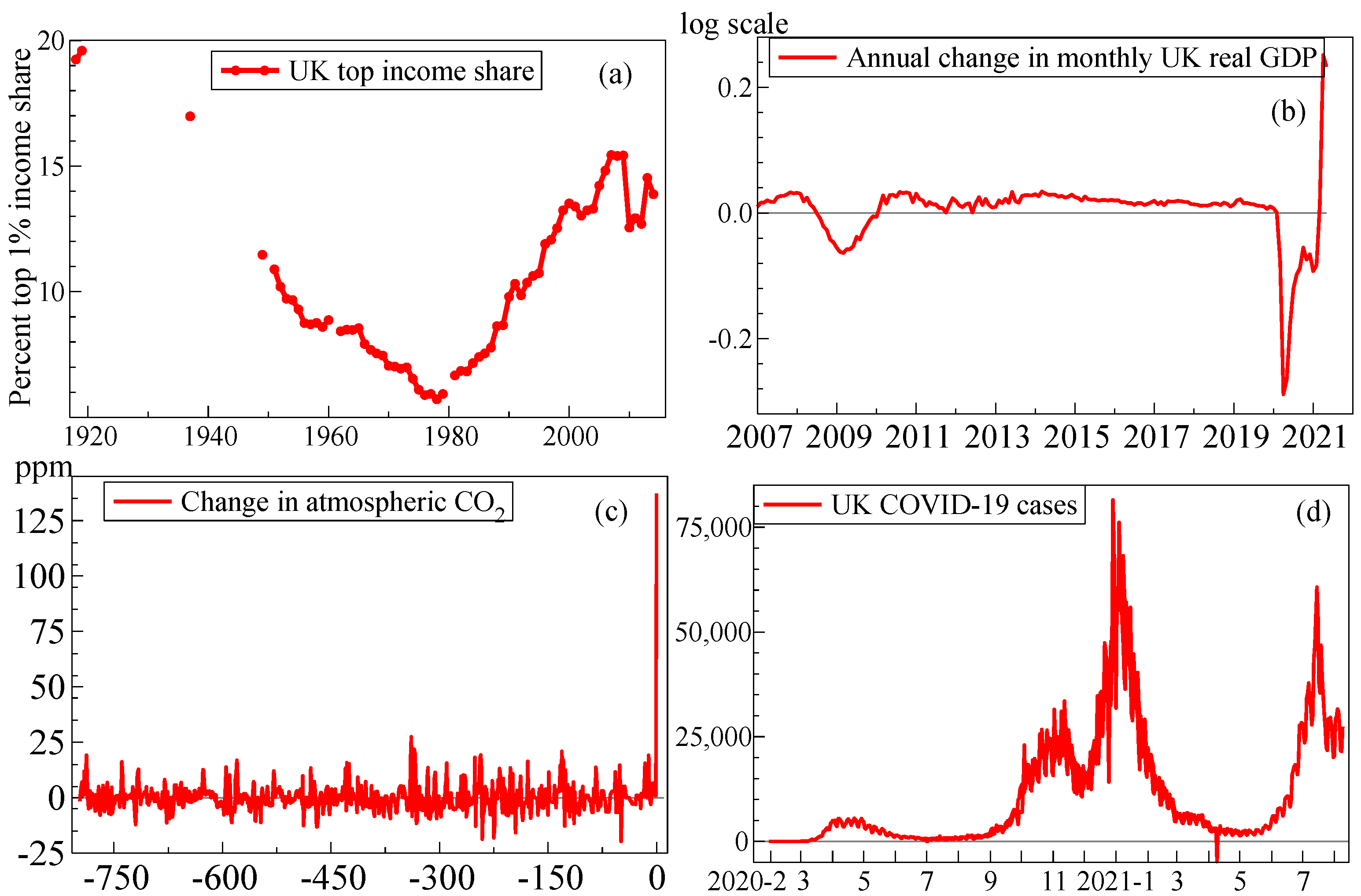
Figure 1a–d illustrates the magnitudes of some of these sudden shifts. Panel (a) emphasises the long-run prevalence of wide-sense non-stationarity illustrated by top income shares in the UK since 1918, exhibiting changing trends, with a systematic fall in income inequality until 1979 and a subsequent reversal of that trend in the Thatcher era that continued until the 21st century. The huge drops in UK real GDP and hours worked seen in Panel (b) resulting from the lockdowns during the pandemic dwarf any previous recorded values, including the ‘Great Recession’, but are followed by a massive rise. In the UK, the Coronavirus Job Retention Scheme, or furlough scheme, prevented the concomitant increase in unemployment that was forecast by some models (see Castle et al. 2021d). On a very different time scale, Panel (c) reports the massive increase of almost 140 parts per million (ppm) in atmospheric CO in just the past 250 years compared to the ppm 1000-year variations over the last 800,000 years of eight Ice Ages advancing and receding. Finally, Panel (d) records the large changes in reported UK new confirmed cases of COVID-19 infections, with four apparent ‘waves’ of varying magnitudes and durations, partly due to more or less intensive testing and changing coverage but also revealing some ‘negative’ numbers due to recording errors.
Polutant emissions like NOx have also changed considerably, and very differently across countries as Gaubert et al. (2021) document. Moreover, Le Quéré et al. (2020) show that global CO emissions fell sharply as lockdowns were mandated in many countries: Liu et al. (2021) provide an update. We return to forecast CO emissions in Section 8.
This small sample of time series in both levels and differences confirms that forecasting practice faces wide-sense non-stationary observed processes in all three disciplines. Changes over time in the distributions of observables occur from stochastic and evolving trends as well as location shifts inter alia. Nevertheless, much of forecasting theory implicitly assumes a stationary world, perhaps after differencing to remove any unit roots. Large shifts can occur in differenced time series as shown in Figure 1b,c, where the change in atmospheric CO seems a relatively permanent jump, and although GDP growth has already recovered, it will drop back again to a more ‘normal’ growth rate.
Different forecasting models seem appropriate in each setting, some well known specifications like autoregressions, random walks, vector autoregressions and simultaneous equations systems, others more recently formulated like, smooth robust predictors, forecasts based on indicator-saturation estimators (which include impulse, step, and trend indicator saturation: IIS, SIS, TIS) and Cardt (Castle et al. 2021a). Cardt is a forecasting device that averages the forecasts from three univariate statistical models, Rho (: a simple autoregressive model), Delta (: in first differences) and THIMA (Trend-Halved Integrated Moving Average). Cardt then treats that set of averaged forecasts as if they were observed to estimate a richer autoregressive model, making it a Calibrated Average, the fitted values from which constitute the final forecasts, discussed more fully in Section 6.
Nevertheless, facing unanticipated future breaks, the fundamental problem remains as to which formulation will continue to provide useful forecasts, so in Section 6, we consider some ‘principles’ that might help avoid systematic forecast failure.
3. Modeling and Forecasting Linear Stationary Processes
It is frequently assumed that the underlying time-series are realizations of a stationary process, perhpas after differencing, so we address this context first.
Introductory statistics and forecasting texts often prove the theorem that the conditional expectation of a variable is the minimum mean square error (MMSE) unbiased predictor: see e.g., (Hansen 2021, chp. 2.11) (or https://en.wikipedia.org/wiki/Minimum_mean_square_error, accessed on 10 August 2021). In econometrics, perhaps even more widely proved is that least squares (OLS) provides the best linear unbiased estimator (BLUE) of a valid linear conditional expectation equation. In economics courses, the law of iterated expectations, namely the expectation of the conditional expectation is the unconditional expectation is widely proved. The precise assumptions required to prove such results are not always fully stated: the first and third rarely state the need for constant distributions, and the second that the parameters of the conditional and marginal distributions must also not be linked.
Under strict stationarity, data distributions are constant, so the expectations operator usually does not need subscripted as the context is clear. Then, incomplete knowledge of the conditioning information does not lead to biased expectations (see e.g., Clements and Hendry 2005b) so conditional expectations can provide unbiased forecasts even from mis-specified, mis-estimated linear models provided the error process has a symmetric distribution. We now consider these results more formally.
Let be a stationary stochastic process with the data generating process (DGP):
The distribution of is unknown and is unpredictable from the full information set with . The linear function is also unknown. Moreover, only the imperfect knowledge information set is available. As is unpredictable from the full information set, it must be unpredictable from any subset thereof, so:
Taking conditional expectations on both sides of (1) using (2):
for some entailed function . Next, let , then from (3):
proving is a martingale difference with respect to . Thus predictions of from are unbiased despite the reduced information set. That proof is subject to knowing , although in practice some selection approach will be needed to discover it, or an approximation thereto.
Let the n dimensional vector denote the observable data that generates , so when , as is linear:
and hence when is independently and identically distributed (i.i.d.) with mean zero and variance . Approximating (4) linearly by using just one component gives the in-sample model as:
where and . When (4) is estimated by:
then .
The 1-step ahead forecasts from (6) from an origin at T are:
leading to the forecast error given by:
The expectation of every term is zero, so , hence the forecasts are unbiased, but will have a larger error variance than . However, in general, so theory testing and policy can go awry despite unbiased forecasts.
Two implications are that evaluating empirical models by forecast performance may not reveal even serious weaknesses (see e.g., Clements and Hendry 2005a); and starting from general information sets (here ) can help avoid under-specifying models.
4. Failures in Modeling and Forecasting from Shifts of Distributions
In practice, stationarity of the underlying time-series processes rarely holds. This is particularly so for the disciplines under consideration involving human behaviour, as illustrated in Figure 1. We consider the implications of unanticipated shifts next.
Even when the in-sample empirical model is an unbiased estimate of the DGP, failure of forecasting, theory, and policy can all occur if the relevant distributions unexpectedly shift. Let be the density of given the DGP information up to time . When in (1) is non-constant:
so that , even keeping i.i.d. . Then expectations need to be subscripted by their time-dependent distributions:
It is misleading sleight of hand not to subscript all expectations by their relevant variables’ distributions when shifts occur, since both integrals in (8) would then be written as:
and hence incorrectly thought to be equal.
Today’s conditional expectation ceases to be an unbiased MMSE predictor of tomorrow’s outcome when distributions experience a location shift. Moreover, when time invariance fails, it is impossible to know either the future , or how the conditioning information would enter the conditional expectation. As a consequence, the law of iterated expectations also fails. To see why, we first note its validity inter-temporally when distributions remain constant over time. If two variables at different dates, say , are drawn from same distribution then:
But when their distributions shift between time periods:
as entails that:
So (10) invalidates inter-temporal results based on the law of iterated expectations after distributional shifts: see Hendry and Mizon (2014) for formal derivations.
The problem highlighted by (8) is the mathematical basis for forecast failure resulting from using the conditional expectation relevant today to forecast what it will be tomorrow. Importantly, (7) is the in-sample DGP up to time t, so even if that was the forecasting model, failure could occur. Moreover, forecast failure is not just a problem for forecasters—it can also entail theory failure. In particular, dynamic stochastic general equilibrium models (DSGEs) are intrinsically non-structural: (9) reveals that their mathematical basis fails when distributions shift—an example is the Bank of England abandoning its quarterly econometric model, BEQEM (see Harrison et al. 2005), after the financial crisis in favour of a new suite of models called COMPASS: see Burgess et al. (2013). Almost all econometric systems in the levels of variables are in fact equilibrium-correction models (EqCMs), including regressions, autoregressions, vector autoregressions, simultaneous equations and cointegrated systems, ARCH, and GARCH as well as DSGEs, all of which converge back to their in-built equilibria irrespective of shifts therein. Consequently, after location shifts, all EqCMs must be adapted to avoid systematic forecast failure.
These results are not unique to linear models. There are infinitely many non-linear models with embedded equilibria (including DSGE). Structural breaks are just as pernicious in non-linear models and suffer the difficulty of identification between non-linearities and structural breaks. This will exacerbate forecasting difficulties making the detection of breaks even more important. If the underlying DGP is linear with structural breaks but is treated as non-linear then forecasts will embed this misspecified non-linearity leading to poor forecasts. Conversely, if the DGP is non-linear but is treated as linear with breaks then forecasts will not reflect the non-linearity present, for example in the form of missed regime switches. Crucially, methods to detect structural breaks such as indicator saturation estimation can be applied to non-linear models, allowing a data-based method of identification between breaks and non-linearities. We proposed a general low-dimensional test for non-linearity in Castle and Hendry (2010), and addressed issues of non-linear model selection facing (e.g.,) outliers in Castle et al. (2021b).
5. The Optimum: Forecasting Breaks in Advance
We have argued that stationarity is often invalidated by shifts in distributions from structural breaks. This leads to forecast failure, often over a long period if models keep moving back to the previous built-in equilibrium. This section considers forecast adjustments once it is suspected that a break has occurred, as well as the possibility of forecasting a break.
A relevant example is the Indian Ocean tsunami on 26 December 2004, caused by an undersea earthquake. In relation to this, Castle et al. (2011) discussed the necessary conditions for usefully forecasting breaks before they occur:
- (i)
- the break in question is predictable;
- (ii)
- there is information relevant to that predictability;
- (iii)
- such information is available at the forecast origin;
- (iv)
- there is a forecasting model specification that embodies it;
- (v)
- there is a method for selecting that model from observations;
- (vi)
- the resulting forecasts are usefully accurate.
They note that, although the exact timing of the tension release at the subduction zone that triggered the earthquake was unpredictable, the devastating consequences of the resulting tsunami could have been predicted: the satellite, Jason-1, measured the existence of the tsunami by altimetry 2 h after it started, so warnings could have been issued to some areas which were later affected, but the data were not analyzed till several days later.1 Treating the break as the tsunami hitting Sri Lanka, and using the empirical tsunami models developed for Hawaii, then (i)–(vi) seem to be satisfied, albeit unfortunately only after the event in this instance. An Indian Ocean tsunami early warning system is now in place: see https://tsunami.incois.gov.in/TEWS/searlywarnings.jsp (accessed on 1 September 2021).
An everyday example of conditions (i)–(vi) in operation is when a trustworthy garage mechanic ‘forecasts’ that your car’s brakes are about to fail and need changing, advice it is usually worth taking to avoid a serious accident. The mechanic knows that (i) unsafe brakes will not stop the vehicle; (ii) has checked the brake discs and found that they are worn; and (iii) knows that information now; (iv) the ‘model’ is that brakes are essential to stopping; and (v) that model has been verified all too often; and (vi) would happen again if new brake discs are not fitted. Paradoxically, the forecast would not actually materialize if the brakes were in fact repaired. An instance of this was the millenium bug (Y2K), resulting from the fact that years where coded with two digits in the early days when computer memory was very limited. Then year 2000 (coded as 0), would be before 1999. A major campaign successfully prevented the predicted Y2K systems’ meltdown, leaving space for dissenting opinions. Similarly, the US public health response to the 2009 H1N1 influenza pandemic (swine flu) was relatively effective, and may have led to some subsequent lowering of the guard, although this is dwarfed by the ineffective and misleading response to the COVID-19 pandemic of the Trump administration (see several recent leaders in The Lancet).
A different notion of forecasting a break occurs in predicting the rebound in temperature after a volcanic eruption. Applying designed break-indicator saturation using a shaped indicator to annual time series of temperature reconstructions, Pretis et al. (2016) show that past major volcanic eruptions can be detected. Immediately after locating the temperature drop following an eruption, a single observation on the indicator value can then forecast the change in direction of the temperature recovery and provide a close approximation to the subsequent trajectory. Again, conditions (i)–(vi) are satisfied.
Next, the impact of the COVID-19 pandemic on various European countries was clearly predictable using the explosion of cases and deaths in Italy in mid-February 2020 as a leading indicator satisfying (i)–(iii), which could be used even though there was no previous history for model estimation: see e.g., Harvey (2021). Unfortunately, the UK government failed to take any action till mid-March, when it was far too late to avoid large numbers of deaths: see Aron and Muellbauer (2020). Thus, a new item must be added to the list:
- (vii)
- the forecasts are acted on in a timely and effective way.
Our short-term forecasts of COVID-19 cases and deaths are discussed in Section 9.
While the terrible health and economic costs of the pandemic are of a magnitude not seen since the ‘Spanish’ flu outbreak a century ago, failures to forecast breaks are legion: economic forecasting has long been prone to miss shifts of distributions. The sudden onset of the Great Depression starting in October 1929 was not forecast (except perhaps by Roger Babson: see Friedman 2014), possibly vindicated by Dominguez et al. (1988) still being unable to forecast the sharp downturn using modern approaches. Failures to forecast ‘turning points’ are common: see e.g., Stekler (1972) for an early study and An et al. (2018) for a follow up.2 The Financial Crisis of 2008 was not predicted, and as the UK’s Queen famously asked, ‘why not?’. However, in this case there was not a single easily observable trigger event such as an earthquake or volcanic eruption. But extreme events such as the bank run on Northern Rock in September 2007 and the collapse of Lehman Brothers exactly a year later provided warning signals.
Although distributional shifts are an important source of non-stationarity in observational time series (also see the evidence on shifts in economic time series in Stock and Watson 1996; Clements and Hendry 2001), they are rather less studied than stochastic trends and unit roots where the literature is vast. By definition, forecasts are almost bound to go awry facing unanticipated distributional shifts, like the initial onset of the COVID-19 pandemic, failing (ii) and (iii). All too often, however, forecasts unnecessarily remain persistently wrong well after the shift has become apparent, such as the Office for Budget Responsibility (OBR) forecasts of UK productivity which were seriously wrong for 15 years, or Surveys of Professional Forecasters (SPF) that have consistently over-predicted U.S. Treasury bond yields for the past 25 years, as discussed by Martinez et al. (2021).
6. Some ‘Principles’ for Specifying Forecasting Models
A stationary context provides us with provable optimality theorems about forecasting, with, in general, better models leading to better forecasts. Allowing for wide-sense nonstationarity (which comes in many forms) takes these all away. Then using a simple autoregressive model, or a no-change (random walk) forecast, can be difficult to improve upon. We now consider a set of principles that can guide us through the forecasting process. Cardt and forecasting devices robust after shifts are introduced.
There ought to be unanimous agreement that stationarity is not a viable basis for deriving theoretical forecasting results of relevance to empirical practice. Nor is it necessary, as discussed in Section 4. Recurring bouts of systematic mis-prediction have led to a lack of consensus about ‘good’ forecasting methods, exacerbated when an advantage claimed by one approach disappears when forecasting over other time periods or different variables, as discussed by Castle et al. (2021a). ‘Structural’, or theory-based, formulations play important roles in understanding in most disciplines, but structural model-based forecasts have indifferent to poor forecasting records. As almost all forecasting models are equilibrium-correction models, handling location shifts in all three disciplines’ models of observational times series improves forecasts. Nevertheless, poor forecasts do not always entail invalidity of ceteris paribus theoretical analyses: the failure of Apollo 13 to reach the moon at the forecast time did not invalidate Newtonian gravitational theory.
There are two solutions to avoiding systematic forecast failure after shifts: adapt theory-based systems, or use predictors that are robust to such shifts.
Combining the insights from their research, the forecasting literature, the M3 and M4 forecasting competitions and forecasting the COVID-19 pandemic (see Doornik et al. 2020b, 2021), Castle et al. (2021a) suggested eight general ‘principles’ that could guide the specification of models primarily intended for forecasting potentially wide-sense non-stationary time series. Here we add two further principles:
- (I)
- address ‘special features’ like seasonality;
- (II)
- adapt the choice of predictors to the data frequency;
- (III)
- select variables in forecasting models at a loose significance;
- (IV)
- dampen trends and growth rates;
- (V)
- shrink estimates of autoregressive parameters in small samples;
- (VI)
- average across forecasts from ‘non-poisonous’ methods;
- (VII)
- include forecasts from robust devices in that average;
- (VIII)
- update estimates as data arrive, especially after forecast failure;
- (IX)
- do not expect any single method to dominate at all times;
- (X)
- check the implied trend when modeling in differences.
The nature of the M4 competition (see Makridakis et al. 2020) precluded analyzing (II), (III), and (VIII), and also adapting the choice of predictors to multivariate contexts. Castle et al. (2021c) investigate (III), and show that even in processes with location shifts occurring at or after the forecast origin, loose selection significance levels similar to Akaike (1973) (AIC, so 10–16%) perform best. However, when using indicator saturation estimation, which involves selecting over more variables than observations, tighter significance levels seem advisable.
Implementing (VIII) in a system context matters even more as location or trend shifts in unmodeled included variables alter collinearity which can greatly increase root mean square forecast errors, whereas rapidly updating estimates as new data arrive usually offsets that problem. Data revisions also require that estimates are updated. Occasionally the ‘past’ is changed significantly (e.g., with GDP or COVID-19 data), with substantial impacts on estimated models. This can also affect perceived forecast accuracy, although it is outside the control of the forecaster.
(VII) is more important if we are confident that a break has occurred, and the forecast model is equilibrium correcting (most models are): in that case we may wish to give much larger weight to robust forecasts. Robust forecasts can be obtained by applying the difference operator to both sides of the estimated model to obtain forecasts of the changes, which are then added to the last observed level. A different, but related, approach is presented in Martinez et al. (2021).
There is ample evidence supporting (IX). In M4, e.g., the method that was best for annual data did not do so well with hourly data (which may also be caused by (I)). Castle et al. (2021a) also have several graphs where rankings change when the sample is extended. This suggests that trying to find the ‘one method that beats them all’ is fruitless. It is now also well known that two different scalar measures of forecast accuracy can give different rankings: see Clements and Hendry (1993).
(X) is relevant when the model implies trending behaviour, but that trend may change. It also pays to check the adequacy of differenced-data models by deriving levels forecasts.
We developed the Card method for the M4 forecasting competition which required 100,000 forecasts of various univariate time series across a range of frequencies and time-series properties. A small subsequent extension was made to result in Cardt, see Doornik et al. (2020a) and Castle et al. (2021a). Cardt is based on the principles of robustness, trend dampening, flexible seasonality, calibration, and averaging. The method estimates three univariate time-series models including Rho (), Delta () and THIMA. estimates a first-order autoregressive model with seasonality, forcing a unit root when estimates are close to unity, in which case it then switches to a first-difference model with a dampened mean; estimates the growth rate from first differences, but dampened by removing large values and allowing for seasonality; THIMA fits a trend-halved integrated moving average model, namely a dampened trend arbitrarily halved, with an intercept correction estimated by a moving-average model. Next, we compute the arithmetic average of these three forecasts. The resulting average forecasts are treated as if they were observed data and a richer autoregressive model is estimated from the extended data series. This is what is termed the Calibration stage. The fitted values from this calibrated model are the final forecasts, undoing any transformations such as logs and differencing (higher orders of integration such as I(2) and damped I(2) were added for the COVID-19 data). The calibration stage is crucial as it allows for a richer autoregressive model to be estimated, providing a better approximation to the time-series properties of the data, without concerns about overfitting or explosive roots because the new model is not used to extrapolate forecasts. Instead, the forecasts are the fitted values from the updated autoregressive model incorporating the first stage average forecasts, and hence have stable properties over the forecast horizon. (X) is addressed by an attempt to detect persistent bias in the calibration residuals at the end of the sample.
7. Forecasting Facing Shifts in Economics
Shifts in distributions affect our ability to forecast. Three empirical applications illustrate the relevance of the principles when forecasting within the three disciplines, starting with economics, followed by climate and finally the COVID-19 pandemic. The first application shows that using a trend in the forecast model, when in fact that trend has changed, can lead to persistent forecast failure.
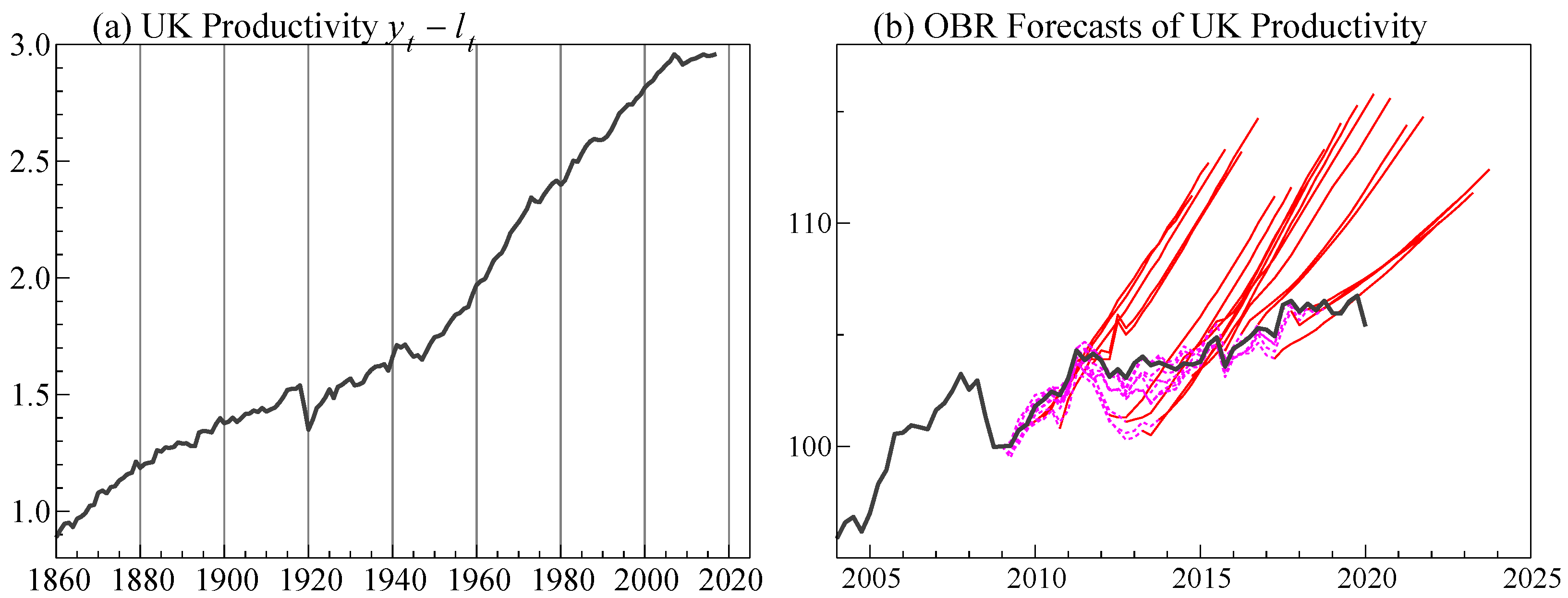
Figure 2a shows the historical time-series of UK productivity, together with 15-years of 5-year ahead forecasts by the Office for Budget Responsibility (OBR) in part (b). We aim to show how a misrepresented structural trend can give rise to such persistent mis-forecasting, using trend indicator saturation (TIS: Castle et al. 2019) to detect trend shifts in a long-run UK production function. TIS can also help to resolve a puzzling empirical relation concerning the coefficient of capital per worker if a constant trend is assumed to represent ‘disembodied’ technical progress.
The data consists of Y, L, and K, where Y is GDP(A) at factor cost and constant prices, L is working population minus unemployment, and K is total gross capital stock, from 1860 to 2017: Hendry (2015) provides details of the data. Lower case letters denote natural logarithms, and is a deterministic trend, with plotted in Figure 2a.
First, assuming a constant trend, the estimate of the empirical production function over almost a century and a half (up to 2007) delivers:
In (11), coefficient standard errors are shown in parentheses, is the residual standard deviation, is the coefficient of multiple correlation, tests for residual autocorrelation (see Godfrey 1978), tests for autoregressive conditional heteroscedasticity (see Engle 1982), tests for residual heteroskedasticity (see White 1980), tests for non-Normality (see Doornik and Hansen 2008) and tests non-linearity (see Ramsey 1969). One star indicates test significance at , two at .
Model (11) uses contemporaneous information in the predictive model (capital per worker) which allows the effect of the trend estimates to be isolated to explain forecast performance. However, the coefficients of and the trend are implausible: the former suggests that the share of labour was merely 23%, inconsistent with direct measurements, and the trend growth in other sources of productivity was just 0.2% per annum. Since every mis-specification test is significant at any reasonable significance level, the estimated standard errors are unreliable. Moreover, methods such as heteroskedastic and autocorrelation consistent standard errors (HACSEs) are unlikely to be useful either, as an important component of the mis-specification rejections is almost certainly due to trend breaks clearly visible in Figure 2a.
TIS saturates a model with trend indicators from which significant trends are retained using a multi-path block search algorithm, capturing broken trends at any unknown points in the data sample. TIS is a variant of indicator saturation, see Johansen and Nielsen (2009), where the trends are defined as , through up to , implemented in Autometrics (see Doornik 2009). We also apply step indicator saturation (SIS) jointly, allowing for level shifts to be detected in a more parsimonious form, see Castle et al. (2015). Both forms of saturation include as many indicators as observations (excluding any that are perfectly collinear with the intercept and full sample trend as these are included but not selected over), so selection must be done at very tight significance levels to avoid overfitting (measured by the retention of irrelevant indicators, called the gauge). At such tight levels the fraction of irrelevant indicators is very close to the selection significance level so there is almost no chance that broken trends or step shifts are detected in (12) when they are irrelevant.
Using a selection significance level of yields:
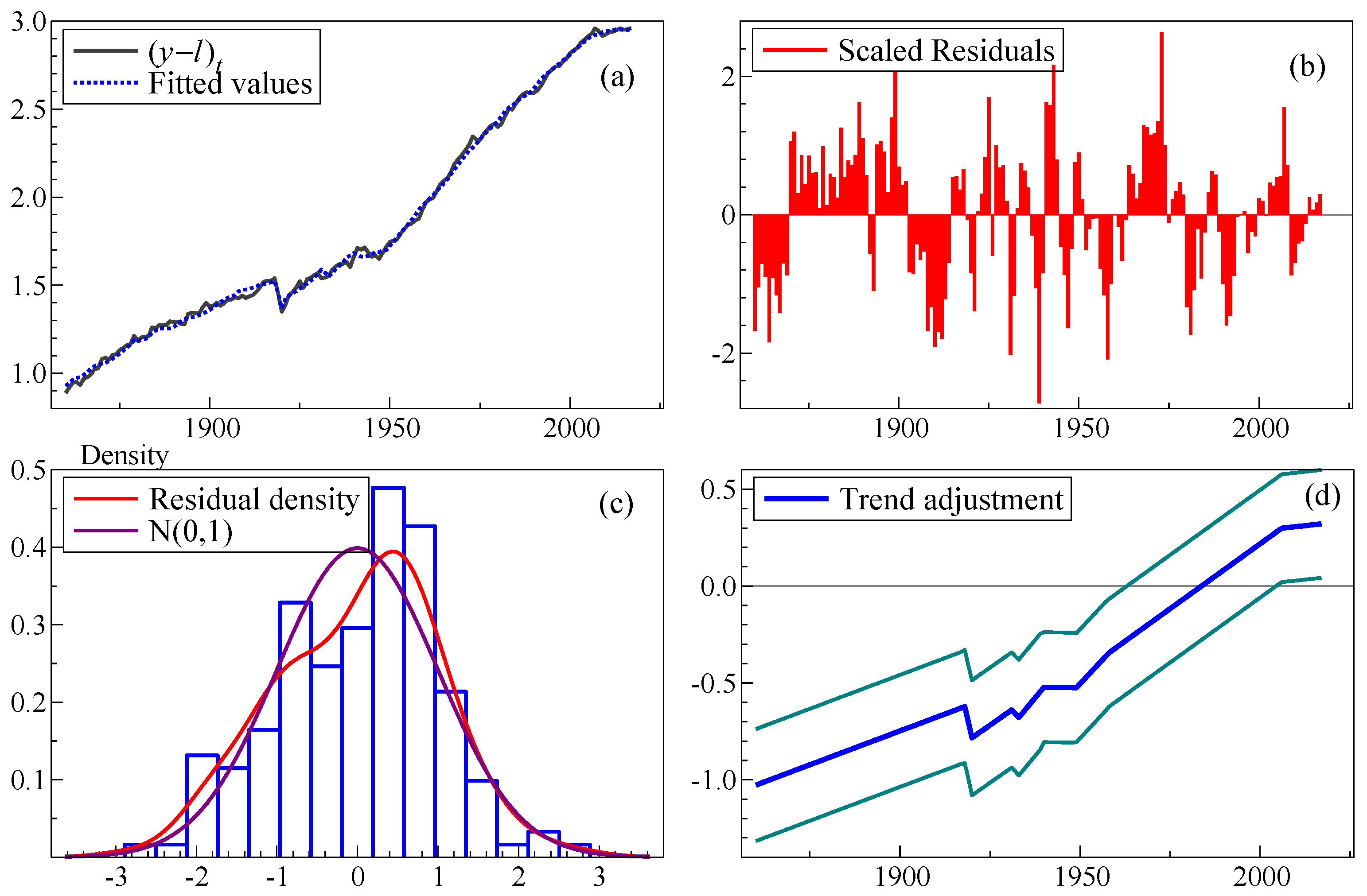
Heteroskedasticity and autocorrelation robust standard errors (HACs) are reported in parentheses. The model is estimated over the full sample up to 2017: the main point is to show the need for different trends. Eight trend shifts are retained (all scaled by 100), with no step shifts, and the coefficient of is now plausible at 30%. The shift in 1919 essentially cancels that of 1917, as does the shift in the early 1930s and that of 1948 cancelling the shift in 1939 over World War II. The trend rate of productivity growth was 0.7% up to WWII, increasing to 1.3% in the interwar period and no growth throughout WWII. Then in 1948 with the post-war reconstruction and Beveridge reforms, trend productivity increased to 2% p.a., tailing off in 1957 to 1.3% before flattening completely in 2005 to productivity growth at just 0.02% p.a. The outcome is recorded in Figure 3.
Equation (12) could be generalized to include dynamics in the form of lagged output per worker and capital per worker. This will resolve the misspecification present in the model, but will obscure the emphasis on breaks in trends. Including dynamics will mean the lagged dependent variable can proxy the shifts in trend through a coefficient close to one. Excluding dynamics enables trend saturation to model the shifts directly. To enable comparisons between (11) and (12) we do not include dynamics to enable direct estimation and extrapolation of a static production function.
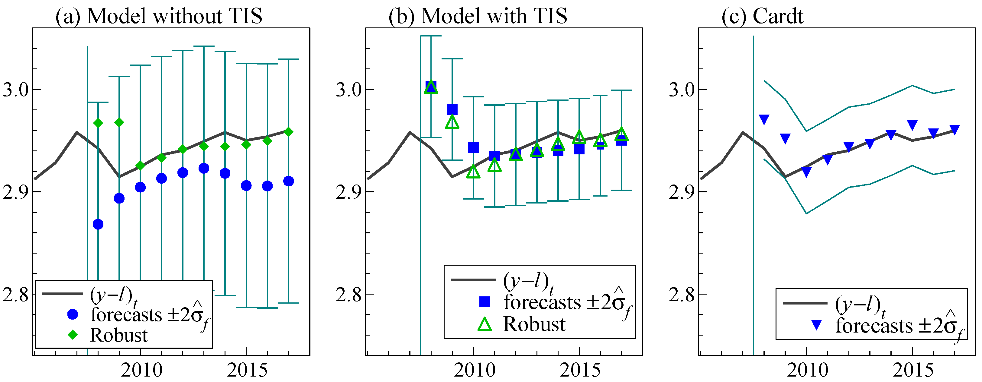
The 1-step ahead pseudo forecasts are computed for models (11) and (12), and reported in Figure 4 and Table 1. Forecasting starts in 2008, using recursive estimation, i.e., re-estimating the model each time, but keeping the structure fixed. These are not ex ante forecasts, because we condition on and performed the TIS selection over the full sample up to 2017. We also report the results from the robust version of (11) and (12) from Hendry (2006) along with the 1-step ahead forecasts computed from Cardt. The robust versions of the production functions difference both sides of the equation without re-estimating which removes the constant term and changes the trend into a constant. The forecasts are then re-integrated by adding the previous level, noting that trend indicators end at 0 so will not enter the forecasts; for example, the forecasts for (12) would be given by .
The forecasts of output per worker without modeling the trend breaks are substantially worse than the forecasts when the trend breaks are modeled, with RMSEs more than 60% larger. A break in trend very close to the forecast origin is detected by TIS () which leaves only one observation to identify the break when estimating up to 2007 given the intercept and full sample trend forced in the model. The standard errors on both and the full sample trend fall from 2.6 to 0.7 with two further observations up to 2010. Hence, the implied trend is very uncertain immediately after the break, as can be seen in Figure 4b for the forecasts in 2008/9. After two periods, the broken trend is accurately estimated and the forecasts based on TIS improve dramatically, falling from a RMSE of 3 to 1.13 by removing the 1-step ahead forecasts for 2008 and 2009.
The robust forecasts applied to the TIS selected model are very similar to the TIS based forecasts which indicate there is no systematic bias in the TIS forecasts. Figure 4b shows that all the forecasts from (11) are below the outcomes, so differencing—as implemented by the robust device—is effective. The forecast uncertainty bands are also significantly smaller for the TIS forecasts, highlighting the importance of modeling trend breaks for forecasting. Both the robust predictor and Cardt (described in Section 6) improve on the forecasts modeling the breaks using TIS, confirming their effectiveness in rapidly adapting to breaks.
While models (11) and (12) are not proper forecasting models (unlike Cardt), the results illustrate how forecasts can go wrong systematically. Shortly after the break, when there is not enough information yet to estimate the new trend, forecast methods that are robust provide a useful complement to the existing model. TIS can help to detect such breaks.
8. Forecasting Changes in CO Emissions over the Pandemic
Our climate forecasting example considers reductions in CO emissions over the COVID-19 pandemic. This intrinsically involves all three disciplines.
To limit the spread of COVID-19 during 2020 and consequential hospitalisations, demands on intensive care units (ICUs) and deaths, many countries and regions suddenly imposed lockdowns and other non-pharmaceutical interventions (NPIs). The restrictions on travel and key aspects of economc activity led to reductions in CO emissions. Lockdowns were imposed at different points in time in early 2020 across countries, for different geographical coverages and stringencies. Lockdowns have continued during 2021, but our data are for 2019–2020, before effective vaccines were available.
Behavioural changes also occurred, with voluntary isolations and social distancing having similar impacts on economic activity. Various economic policies, such as job retention schemes or ‘furlough’ schemes, sought to minimize the economic damage by changing economic relationships without worsening the pandemic, and again were at different levels of generosity and coverage for different time periods in different countries: see Castle et al. (2021d). Consequently, differential levels of CO emissions compared to the same date in 2019 had many shifts, making forecasting especially difficult, putting a premium on predictors that are robust after breaks.
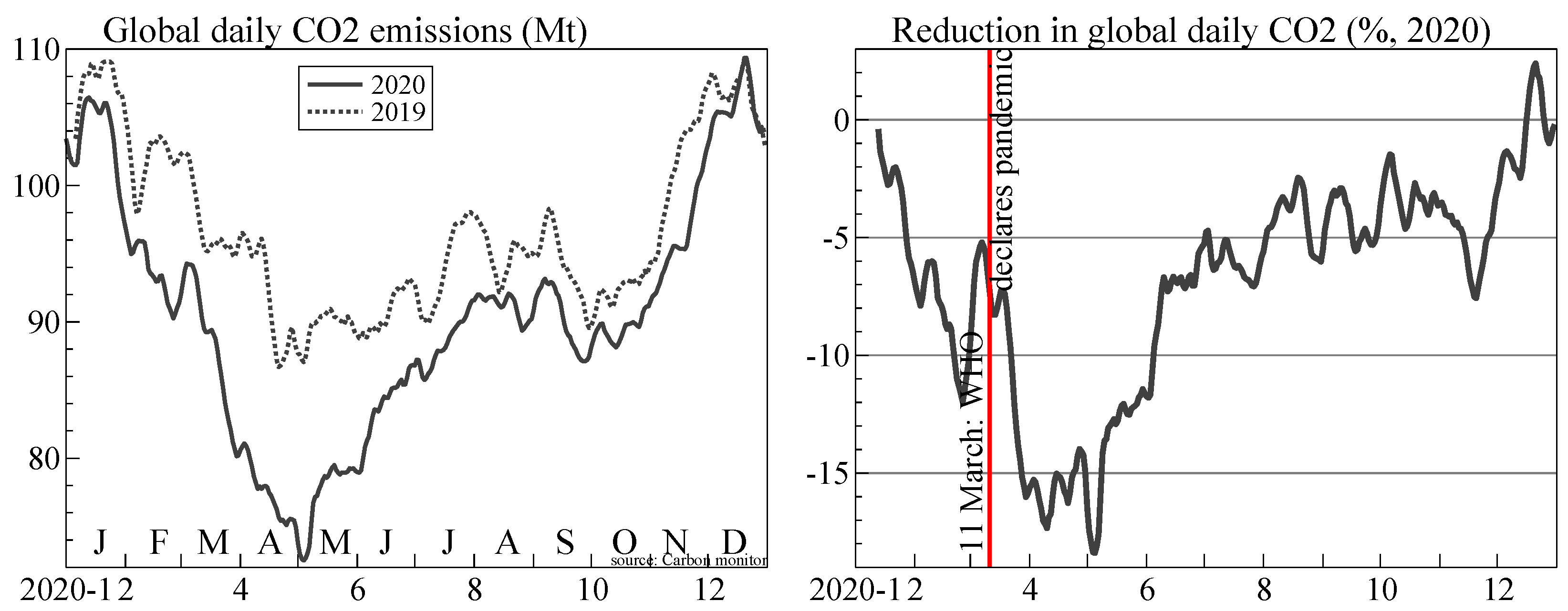
Figure 5 shows the reduction in global CO emissions during 2020 based on daily data available from https://carbonmonitor.org (accessed on 24 September 2021): see Liu et al. (2021) for a detailed description. On the left are global daily emissions, as an average over the last seven days to remove seasonality within the week. As a contrast, the dotted line shows the data for 2019 (using a lag of 52 weeks, 364 days). On the right is the percentage change in 2020 from the previous year. In that case, we use more smoothing in the denominator: the 2019 data are an average over three weeks, centered on the same week as used for 2020. The sharp drop in March 2020 is clearly visible, and during April emissions were down by , albeit a tiny reduction of under 20 Mt relative to annual emissions of more than 3 ppm (1 ppm = gigatonnes).
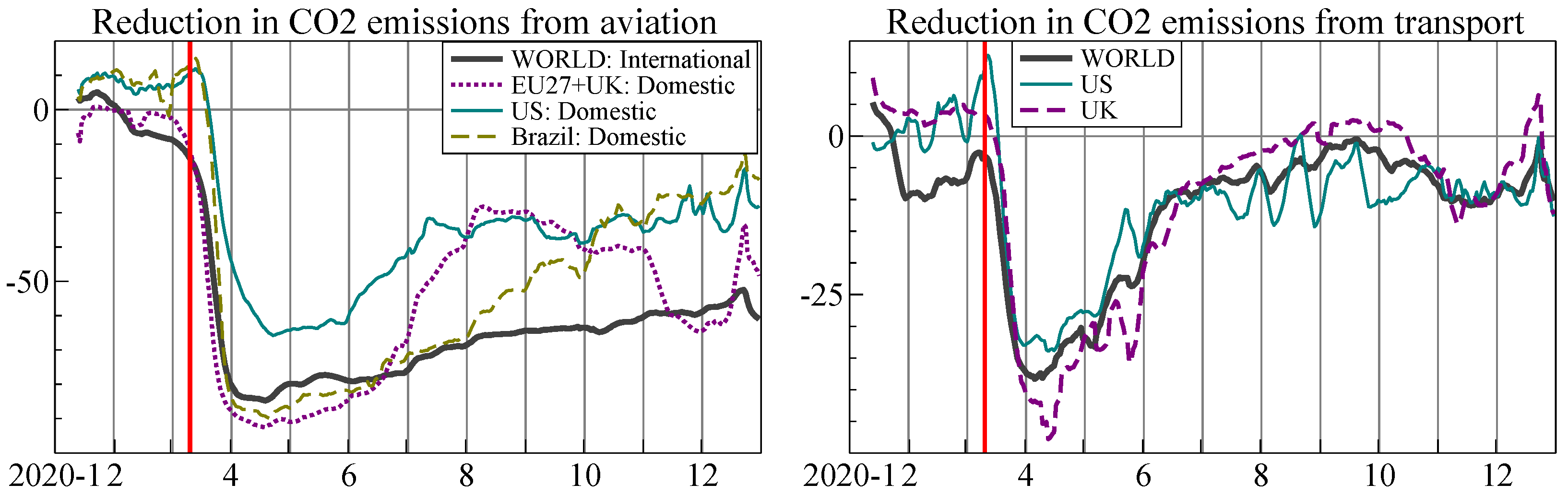
Figure 6 shows the reductions in emissions from aviation and ground transportation, which were particularly affected by the lockdowns. The drop from transportation has largely disappeared by September 2020, although COVID-19 cases surged again in many regions towards the end of the year. Emissions from international aviation remained low: many travel restrictions have persisted into the second half of 2021.
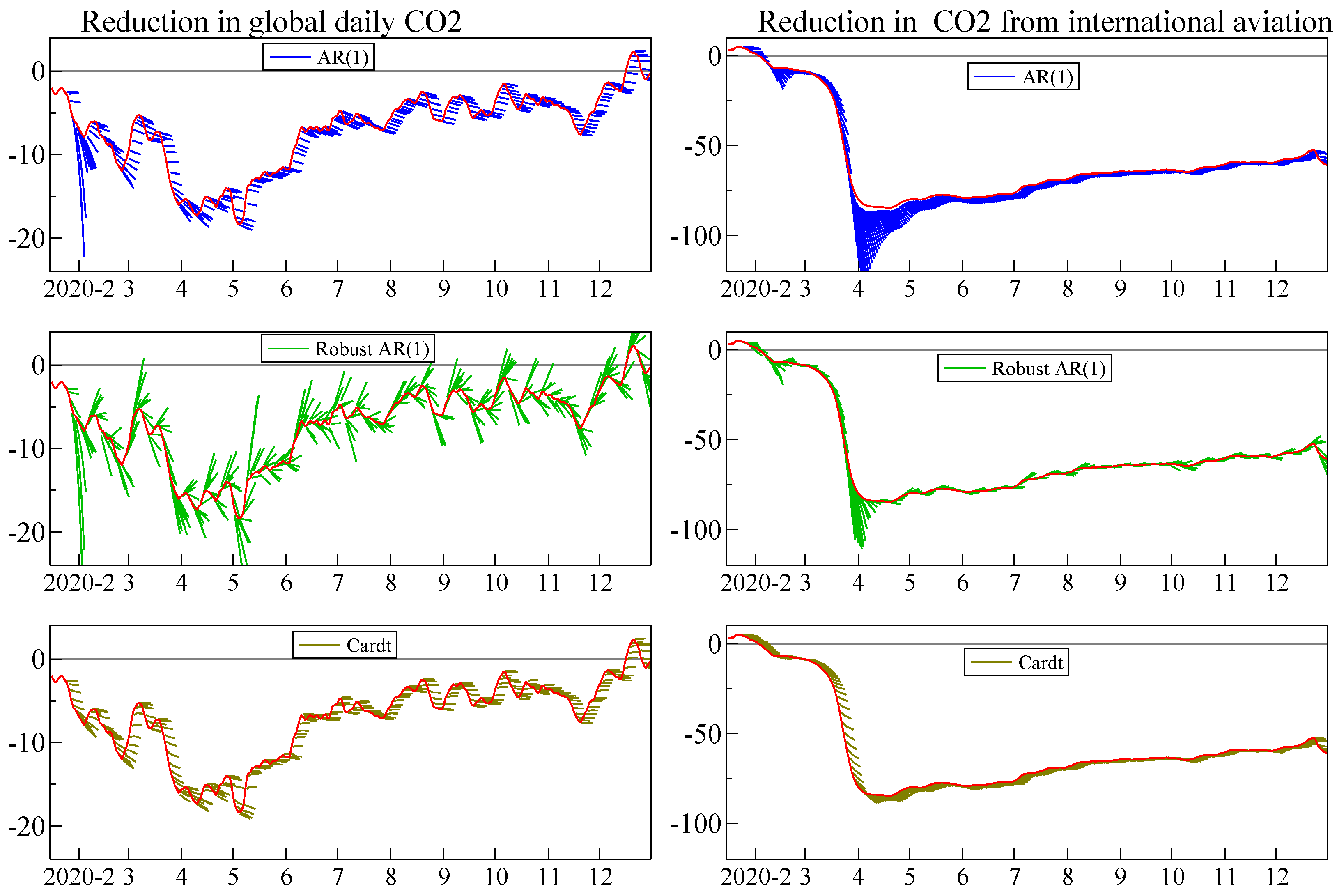
Figure 7 shows so-called hedgehog graphs: each short line is a seven day out-of-sample forecast using updated parameter estimates. The three forecasting devices we applied for 1 through 7 days ahead are an autoregression of order one with an intercept: AR(1); the robust AR(1), also written as RobAR1; and Cardt. We use data from 16 January 2020 to 31 December 2020, and the first forecast is for 24 January based on just 8 observations. Table 2 reports the relative RMSEs and MAPEs of the methods compared to the benchmark AR(1) model.
The robust transformation of the AR(1) model, as described in Section 6, has the smallest RMSE and MAPE one step ahead. Two steps ahead, Cardt starts to get closer to the robust forecasts, with mostly smaller RMSE and MAPE seven days ahead. For global CO emissions, the AR(1) and its robust version go awry in early February: this is (V) in action, but Cardt is robust to the small number of observations. Then in aviation at the end of March, the autoregressive model becomes explosive (again: this also happened mid February), which requires protecting against: (IV).
On 7-days ahead forecasts, robust AR(1) does not encompass Cardt, nor vice versa, as shown in (13). Since the 7-day ahead forecasts have at least 6th order moving average errors we report HACSEs in parentheses. For international aviation:
with and for the period 2020-01-31 to 2020-12-31. More results are reported in Table 3.
As advised in (VI) and (VII) above, and often found in practice, averaging forecasts can dominate over the individual best one. Consider averaging robust AR(1), with a diminishing weight on the robust forecasts as the horizon grows:
Choosing gives almost equal weights at 7-steps ahead (). This greatly improves the RMSE of the robust AR(1), often close to halving it, as reported in Table 4. Because of the increasing weights on the Cardt target, the advantage is not always visible at horizon 7.
We also investigate the potential role of (V) for the robust AR(1) predictor, by halving its local forecast ‘trend’, defined as:
This is essentially the smooth robust random walk of Martinez et al. (2021). The target is the last observed value, which is the random walk (or naive) forecast, while the robust forecast shrinks towards this. The difference is that we select , rather than estimate it from a stationary autoregression (which we do not have here). Devices (14) and (15) yield very similar RMSEs. The disadvantage of (14) as given is that it is not yet adapted to seasonality, which is principle (I).
The ranking of methods differs over time, matching the fundamental problem facing forecasters discussed above of having to also forecast which model specification to use at any given time. Switching over time or variables within the ‘best of the bunch’ of forecasting devices in use is not uncommon and supports computing averages, as well as damping both local trends and autoregressive coefficients to avoid the worst outcomes.
9. COVID-19 Pandemic Forecasting
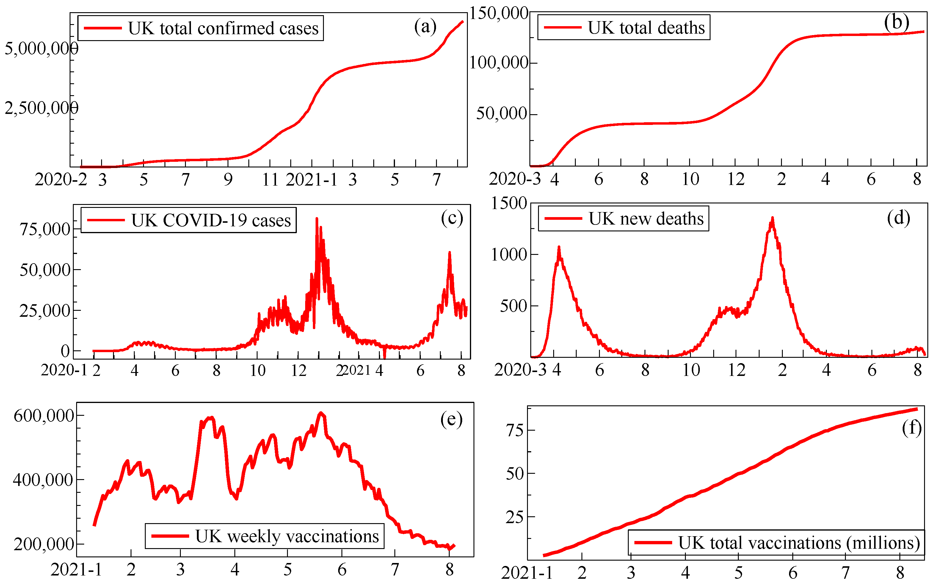
The COVID-19 pandemic, currently dominating the physical and economic well-being of individuals and societies globally (without seriously abating as we write), has put forecasting in the limelight to help plan responses. In addition to its devastating impacts, structural change is a salient feature of the pandemic data: sudden shifts from policy interventions (like lockdowns), evolving technological advances (like testing and vaccines), and rapidly changing trends, as behaviour changes and virus infectivity increases from mutating variants. Data measurement errors that were abruptly corrected, as well as sudden definitional changes and rapid increases in testing all interact with the pandemic process to make the observational time series doubly non-stationary as Figure 8 shows for UK cases, deaths and vaccinations.
Changing definitions in the UK data included the sudden inclusion of care-home deaths, not just those in hospitals, and from having tested positive for COVID-19 at any time to having been caught within 28 days; weekend reporting delays generated unexpected and evolving weekly ‘seasonality’; increased infection rates and antibody testing altered what percentage of cases were recorded, whereas correcting previous reporting errors led to some negative cases (in April 2021); and large revisions occurred when omitted data (due to using an outdated spreadsheet format) were suddenly added back. While some of these features were unique to the UK, others were generic.
Consequently, even short-term forecasting, such as a week ahead, was hazardous. Many variants of epidemiology SIR or SEIR models (susceptible, exposed, infectious, removed), and a number of purely statistical predictors (autoregressions, exponential smoothing, Cardt and growth curves: see inter alia, Petropoulos and Makridakis 2020; Castle et al. 2021a; Harvey and Kattuman 2020) as well as linked economic and SEIR models have all been tried. Examples of the first include the Los Alamos National Laboratory (LANL: see https://covid-19.bsvgateway.org) which has published forecasts twice a week (from 5 April 2020) based on a dynamic growth model, and the Institute for Health Metrics and Evaluation (IHME: see www.healthdata.org) which has published forecasts (since 25 March 2020, but not consistently), combining SIR with curve fitting.
We have produced real-time short-term forecasts of cumulative daily confirmed cases and deaths since mid-March 2020 for ≈50 countries, ≈50 US states, and more than 300 English local authorities. To do so has involved making 4 sets of forecasts about 4 times a week, later forecasting 7 days ahead, so required 3200 model estimates each time. The key to achieving that was automating downloading and sorting data, estimating and forecasting: see www.doornik.com/COVID-19.
To forecast cumulative COVID-19 cases and deaths, we decompose the data into trend, seasonal and irregular components using TIS. Separate forecasts are made of the components before aggregating. The seasonal component is extrapolated from the most recent estimates of the seasonal pattern, whereas the trend and irregular forecasts are computed using Cardt.
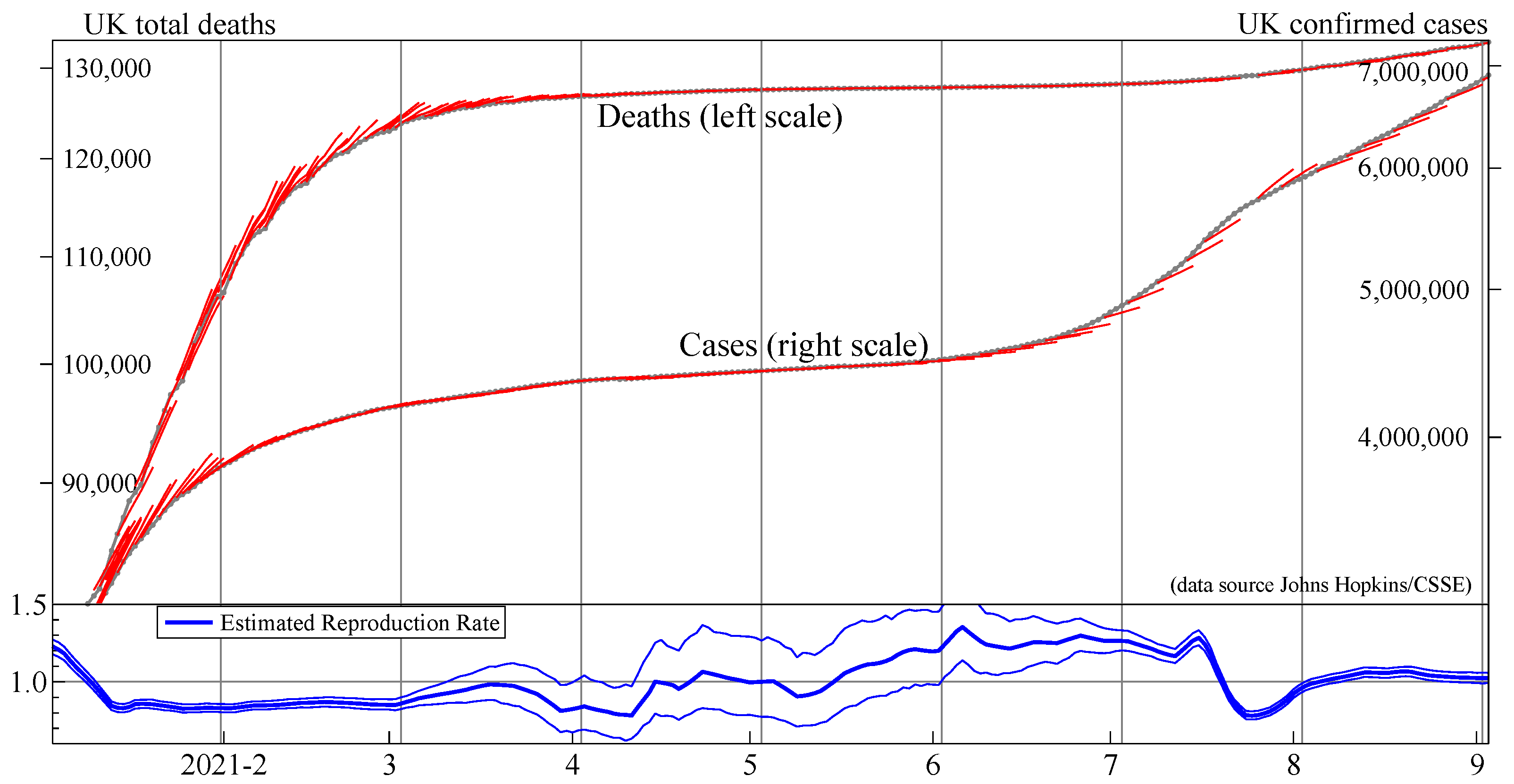
Doornik et al. (2021) evaluate our forecast performance relative to LANL and IHME. Our models produced very good forecasts for deaths, dominating particularly early in the pandemic when little was known about the evolution of the pandemic and agnostic models based on time-series properties of the data performed well. The performance for cases was more average relative to the other forecasting models. Figure 9 records our real-time forecasts for UK total deaths and confirmed cases over January to August 2021. We miss the slow-down in deaths owing to vaccination, as we did not adjust the forecasting model at the time for this structural change.
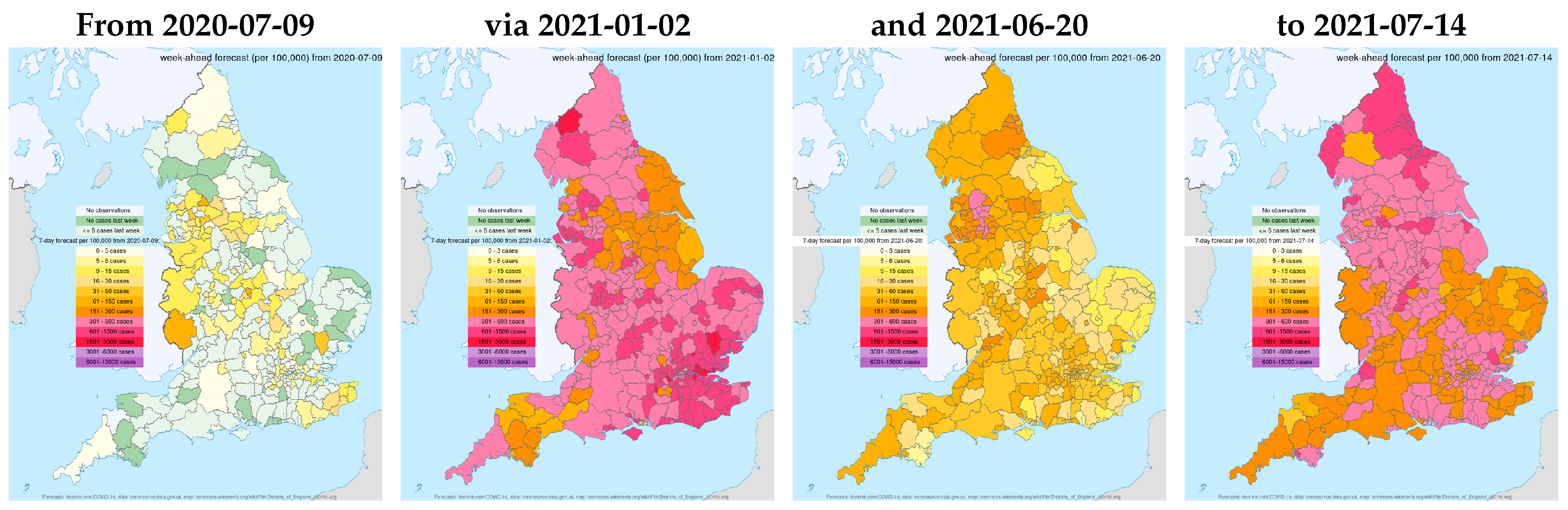
Underlying the aggregate UK COVID-19 statistics, and a feature generally seen worldwide, is changing heterogeneity by locality. Figure 10 highlights this with a sequence of snapshots of our forecasts for Local Authority areas in England. The forecasts highlight the many large regional shifts from widespread low levels in July 2020 after a major lockdown, as well as ‘losing the battle’ in January 2021 following the transition from a tier system during Christmas 2020 to a lockdown early in the new year, starting to win again by June 2021 thanks to the benefits of the rapid development of vaccines and the NHS’s successful vaccination campaign (more than 80 million doses by end August 2021, as seen in Figure 8f), yet partly wasting those victories by mid-July to enable travel for holidays before full protection was achieved. The pattern of cases is also affected by where new COVID-19 variants start, as with the so-called ‘Kent’ (B.1.1.7) mutation, now named alpha, coming in autumn 2020, with delta rapidly becoming dominant during May 2021.
10. Conclusions
Climate change, evolving pandemics and shifts in economic activity all interact. The time-series observations of many variables in all three disciplines are non-stationary from stochastic trends and abrupt shifts, so need robust forecasts to plan over different horizons. The Sars-Cov-2 pandemic has highlighted the complexities of forecasting facing rapidly evolving situations influenced by many, often unknown, factors, yet emphasises the importance of doing so. Moreover, from their common component of human behaviour, all three disciplines have incomplete knowledge of their data generating processes, entailing model search for empirical estimates of ‘structural’ representations, which are essential for understanding, but are not necessarily the best devices for forecasting.
Commonalities across climate, pandemic and economic time series lead to both forecasting similarities and differences across those disciplines. These are partly dependent on the data accuracy and its frequency; partly on the existence of valid conditioning variables and partly on the extent and form of non-stationarity.
We proposed a range of adaptations to forecasting models that experience suggested were helpful in minimizing systematic forecast failure. ‘Principles’ from Section 6 that were useful in the applications included (VIII) (update estimates as data arrive, especially after forecast failure) and (X) (check the implied trend), implemented through trend indicator saturation, and relevant in Section 7. Next, (IV) (dampen trends and growth rates), (VI) (average across forecasts from ‘non-poisonous’ methods), (VII) (include forecasts from robust devices in that average, (VIII) (update estimates as data arrive) but jointly with (V) (‘shrink’ estimates of autoregressive parameters in small samples) were all useful in Section 8, which also implemented (X) by using robust predictors in differences that were transformed back to levels as proposed. Section 9 highlighted the role of (I) to address the ‘special feature’ of seasonality, as well as the value of robust predictors.
Applications in each arena illustrated and compared forecasting devices stressing the difficulties of forecasting but seeking viable approaches. Sudden shifts are naturally often unanticipated, as with the onset of COVID-19, and hence almost unpredictable. Consequently, we have focused on forecasting devices that are relatively robust after such shifts, and hence help avoid systematic forecast failure.
Author Contributions
Conceptualization, J.L.C., J.A.D. and D.F.H.; Methodology, J.L.C., J.A.D. and D.F.H.; Software, J.A.D.; Formal Analysis, J.L.C., J.A.D. and D.F.H.; Writing and Original Draft Preparation, J.L.C., J.A.D. and D.F.H.; Writing Review and Editing, J.L.C., J.A.D. and D.F.H. All authors have read and agreed to the published version of the manuscript. All calculations and graphs use PcGive (Doornik and Hendry 2021) and OxMetrics (Doornik 2021).
Funding
Financial support from the Robertson Foundation (award 9907422), ERC (grant 694262, DisCont), and Nuffield College is gratefully acknowledged.
Institutional Review Board Statement
Not applicable.
Informed Consent Statement
Not applicable.
Data Availability Statement
Data available from stated sources.
Acknowledgments
We thank Andrew B. Martinez for his comments, and participants at ISF2021, Ecomod2021, and Fifth Econometric Modelling of Climate Change Conferences, as well as three anonymous referees and the editor for their helpful comments.
Conflicts of Interest
Doornik and Hendry have developed Autometrics, which is included in the OxMetrics software package, and have a share in the returns.
| 1 | Retrospectively, Holliday et al. (2006) showed that the high stress tension in that subduction region was measurable before the earthquake. |
| 2 | Also see https://voxeu.org/article/predicting-economic-turning-points, (accessed on 4 October 2021). |
References
- Akaike, Hirotugu. 1973. Information theory and an extension of the maximum likelihood principle. In Second International Symposium on Information Theory. Edited by Boris N. Petrov and Frigyes Csaki. Budapest: Akademia Kiado, pp. 267–81. [Google Scholar]
- An, Zidong, João Jalles, and Prakash Loungani. 2018. How well do economists forecast recessions? International Finance 21: 100–21. [Google Scholar] [CrossRef] [Green Version]
- Aron, Janine, and John Muellbauer. 2020. Measuring Excess Mortality: The Case of England during the Covid-19 Pandemic. INET Working Paper 2020-11. Oxford: Oxford University. [Google Scholar]
- Atwoli, Lukoye, Abdullah H. Baqui, Thomas Benfield, Raffaella Bosurgi, Fiona Godlee, Stephen Hancocks, Richard Horton, Laurie Laybourn-Langton, Carlos Augusto Monteiro, Ian Norman, and et al. 2021. Call for emergency action to limit global temperature increases, restore biodiversity and protect health. The British Medical Journal 374: n1734. [Google Scholar] [CrossRef] [PubMed]
- Burgess, Stephen, Emilio Fernandez-Corugedo, Charlotta Groth, Richard Harrison, Francesca Monti, Konstantinos Theodoridis, and Matt Waldron. 2013. The Bank of England’s Forecasting Platform: COMPASS, MAPS, EASE and the Suite of Models. Working Paper No. 471 and Appendices. London: Bank of England, London. [Google Scholar]
- Castle, Jennifer L., Jurgen A. Doornik, and David F. Hendry. 2021a. Forecasting principles from experience with forecasting competitions. Forecasting 3: 138–65. [Google Scholar] [CrossRef]
- Castle, Jennifer L., Jurgen A. Doornik, and David F. Hendry. 2021b. Robust discovery of regression models. Econometrics and Statistics. [Google Scholar] [CrossRef]
- Castle, Jennifer L., Jurgen A. Doornik, and David F. Hendry. 2021c. Selecting a model for forecasting. Econometrics 9: 26. [Google Scholar] [CrossRef]
- Castle, Jennifer L., Jurgen A. Doornik, and David F. Hendry. 2021d. The value of robust statistical forecasts in the Covid-19 pandemic. National Institute Economic Review 256: 19–43. [Google Scholar] [CrossRef]
- Castle, Jennifer L., Jurgen A. Doornik, David F. Hendry, and Felix Pretis. 2015. Detecting location shifts during model selection by step-indicator saturation. Econometrics 3: 240–64. [Google Scholar] [CrossRef] [Green Version]
- Castle, Jennifer L., Jurgen A. Doornik, David F. Hendry, and Felix Pretis. 2019. Trend-Indicator Saturation. Working Paper. Oxford: Nuffield College, Oxford University. [Google Scholar]
- Castle, Jennifer L., Nicholas W. P. Fawcett, and David F. Hendry. 2011. Forecasting breaks and during breaks. In Oxford Handbook of Economic Forecasting. Edited by Michael P. Clements and David F. Hendry. Oxford: Oxford University Press, pp. 315–53. [Google Scholar]
- Castle, Jennifer L., and David F. Hendry. 2010. A low-dimension portmanteau test for non-linearity. Journal of Econometrics 158: 231–45. [Google Scholar] [CrossRef] [Green Version]
- Clements, Michael P., and David F. Hendry. 1993. On the limitations of comparing mean squared forecast errors (with discussion). Journal of Forecasting 12: 617–37. [Google Scholar] [CrossRef]
- Clements, Michael P., and David F. Hendry. 2001. An historical perspective on forecast errors. National Institute Economic Review 177: 100–12. [Google Scholar] [CrossRef]
- Clements, Michael P., and David F. Hendry. 2005a. Evaluating a model by forecast performance. Oxford Bulletin of Economics and Statistics 67: 931–56. [Google Scholar] [CrossRef]
- Clements, Michael P., and David F. Hendry. 2005b. Guest Editors’ introduction: Information in economic forecasting. Oxford Bulletin of Economics and Statistics 67: 713–53. [Google Scholar] [CrossRef]
- Dominguez, Kathryn M., Ray C. Fair, and Matthew D. Shapiro. 1988. Forecasting the Depression: Harvard versus Yale. American Economic Review 78: 595–612. [Google Scholar]
- Doornik, Jurgen A. 2009. Autometrics. In The Methodology and Practice of Econometrics. Edited by Jennifer L. Castle and Neil Shephard. Oxford: Oxford University Press, pp. 88–121. [Google Scholar]
- Doornik, Jurgen A. 2021. OxMetrics: An Interface to Empirical Modelling, 9th ed. London: Timberlake Consultants Press. [Google Scholar]
- Doornik, Jurgen A., Jennifer L. Castle, and David F. Hendry. 2020a. Card forecasts for M4. International Journal of Forecasting 36: 129–34. [Google Scholar] [CrossRef]
- Doornik, Jurgen A., Jennifer L. Castle, and David F. Hendry. 2020b. Short-term forecasting of the coronavirus pandemic. International Journal of Forecasting. [Google Scholar] [CrossRef]
- Doornik, Jurgen A., Jennifer L. Castle, and David F. Hendry. 2021. Modeling and forecasting the COVID-19 pandemic time-series data. Social Science Quarterly 102: 2070–87. [Google Scholar] [CrossRef]
- Doornik, Jurgen A., and Henrik Hansen. 2008. An omnibus test for univariate and multivariate normality. Oxford Bulletin of Economics and Statistics 70: 927–39. [Google Scholar] [CrossRef]
- Doornik, Jurgen A., and David F. Hendry. 2021. Empirical Econometric Modelling Using PcGive: Volume I, 9th ed. London: Timberlake Consultants Press. [Google Scholar]
- Engle, Robert F. 1982. Autoregressive conditional heteroscedasticity, with estimates of the variance of United Kingdom inflation. Econometrica 50: 987–1007. [Google Scholar] [CrossRef]
- Friedman, Walter A. 2014. Fortune Tellers: The Story of America’s First Economic Forecasters. Princeton: Princeton University Press. [Google Scholar]
- Gaubert, Benjamin, Idir Bouarar, Thierno Doumbia, Yiming Liu, Trissevgeni Stavrakou, Adrien Deroubaix, Sabine Darras, Nellie Elguindi, Claire Granier, Forrest Lacey, and et al. 2021. Global changes in secondary atmospheric pollutants during the 2020 COVID-19 pandemic. Journal of Geophysical Research: Atmospheres 126: e2020JD034213. [Google Scholar] [CrossRef]
- Godfrey, Lesley G. 1978. Testing for higher order serial correlation in regression equations when the regressors include lagged dependent variables. Econometrica 46: 1303–13. [Google Scholar] [CrossRef]
- Hansen, Bruce E. 2021. Econometrics. Princeton: Princeton University Press. [Google Scholar]
- Harrison, Richard, Kalin Nikolov, Meghan Quinn, Gareth Ramsay, Alasdair Scott, and Ryland Thomas. 2005. The Bank of England Quarterly Model. Research paper. London: Bank of England, London, 244p. [Google Scholar]
- Harvey, Andrew C. 2021. Time SeriesModeling of Epidemics: Leading Indicators, Control Groups and Policy Assessment. Cambridge Working Papers in Economics CWPE2114. Cambridge: Economics Department, University of Cambridge. [Google Scholar] [CrossRef]
- Harvey, Andrew C., and Paul Kattuman. 2020. Time series models based on growth curves with applications to forecasting coronavirus. Harvard Data Science Review. [Google Scholar] [CrossRef]
- Hendry, David F. 2006. Robustifying forecasts from equilibrium-correction models. Journal of Econometrics 135: 399–426. [Google Scholar] [CrossRef]
- Hendry, David F. 2015. Introductory Macro-Econometrics: A New Approach. London: Timberlake Consultants, Available online: http://www.timberlake.co.uk/macroeconometrics.html (accessed on 15 October 2021).
- Hendry, David F., and Grayham E. Mizon. 2014. Unpredictability in economic analysis, econometric modeling and forecasting. Journal of Econometrics 182: 186–95. [Google Scholar] [CrossRef] [Green Version]
- Holliday, James, John Rundle, Kristy Tiampo, and Donald Turcotte. 2006. Using earthquake intensities to forecast earthquake occurrence times. Nonlinear Processes in Geophysics 13: 585–93. [Google Scholar] [CrossRef] [Green Version]
- Johansen, Søren, and Bent Nielsen. 2009. An analysis of the indicator saturation estimator as a robust regression estimator. In The Methodology and Practice of Econometrics. Edited by Jennifer L. Castle and Neil Shephard. Oxford: Oxford University Press, pp. 1–36. [Google Scholar]
- Le Quéré, Corinne, Robert B. Jackson, Matthew W. Jones, Adam J. P. Smith, Sam Abernethy, Robbie M. Andrew, Anthony J. De-Gol, David R. Willis, Yuli Shan, and Josep G. Canadell. 2020. Temporary reduction in daily global CO2 emissions during the COVID-19 forced confinement. Nature Climate Change 10: 647–53. [Google Scholar] [CrossRef]
- Liu, Zhu, Zhu Deng, Philippe Ciais, Jianguang Tan, Biqing Zhu, Steven J. Davis, Robbie Andrew, Olivier Boucher, Simon Ben Arous, and Pep Canadell. 2021. Global daily CO2 emissions for the year 2020. arXiv arXiv:2103.02526. [Google Scholar]
- Makridakis, Spyros, Evangelos Spiliotis, and Vassilios Assimakopoulos. 2020. The M4 competition: 100,000 time series and 61 forecasting methods. International Journal of Forecasting 36: 54–74. [Google Scholar] [CrossRef]
- Martinez, Andrew B., Jennifer L. Castle, and David F. Hendry. 2021. Smooth robust multi-step forecasting methods. Advances in Econometrics. Forthcoming. [Google Scholar]
- Petropoulos, Fotios, and Spyros Makridakis. 2020. Forecasting the novel coronavirus COVID-19. PLoS ONE 15: e0231236. [Google Scholar] [CrossRef]
- Pretis, Felix, Lea Schneider, Jason E. Smerdon, and David F. Hendry. 2016. Detecting volcanic eruptions in temperature reconstructions by designed break-indicator saturation. Journal of Economic Surveys 30: 403–29. [Google Scholar] [CrossRef]
- Ramsey, James B. 1969. Tests for specification errors in classical linear least squares regression analysis. Journal of the Royal Statistical Society 31: 350–71. [Google Scholar] [CrossRef]
- Stekler, Herman O. 1972. An analysis of turning point forecast errors. American Economic Review 62: 724–29. [Google Scholar]
- Stock, James H., and Mark W. Watson. 1996. Evidence on structural instability in macroeconomic time series relations. Journal of Business and Economic Statistics 14: 11–30. [Google Scholar]
- White, Halbert. 1980. A heteroskedastic-consistent covariance matrix estimator and a direct test for heteroskedasticity. Econometrica 48: 817–38. [Google Scholar] [CrossRef]
Figure 1.
(a) Top 1% income shares in the UK since 1918; (b) annual changes in log monthly UK real GDP since 2007; (c) thousand-year changes in atmospheric CO in parts per million (ppm) over Ice Ages, and last 250 years; (d) UK daily new confirmed cases of COVID-19 to August 2021.
Figure 1.
(a) Top 1% income shares in the UK since 1918; (b) annual changes in log monthly UK real GDP since 2007; (c) thousand-year changes in atmospheric CO in parts per million (ppm) over Ice Ages, and last 250 years; (d) UK daily new confirmed cases of COVID-19 to August 2021.

Figure 2.
(a) UK annual productivity over 1860-2017; (b) Office of Budget Responsibility (OBR) five-year-ahead forecasts of UK productivity.
Figure 2.
(a) UK annual productivity over 1860-2017; (b) Office of Budget Responsibility (OBR) five-year-ahead forecasts of UK productivity.

Figure 3.
(a) Actual and fitted values for from TIS; (b) scaled residuals; (c) residual density and histogram; (d) trend adjustment of the estimated model given the retained trend indicators.
Figure 3.
(a) Actual and fitted values for from TIS; (b) scaled residuals; (c) residual density and histogram; (d) trend adjustment of the estimated model given the retained trend indicators.

Figure 4.
(a) 1-year ahead pseudo forecasts for from model (11); (b) model (12); and (c) 1-year ahead forecasts from Cardt.

Figure 5.
Global daily CO emissions 2019–2020 (Mt, left), and percentage change from 52 weeks before (right). Data from carbon monitor.
Figure 5.
Global daily CO emissions 2019–2020 (Mt, left), and percentage change from 52 weeks before (right). Data from carbon monitor.

Figure 6.
Percentage reduction in daily CO emissions from the previous year: aviation (left) and ground transportation (right). Data from carbon monitor.
Figure 6.
Percentage reduction in daily CO emissions from the previous year: aviation (left) and ground transportation (right). Data from carbon monitor.

Figure 7.
Recursive forecasts of smoothed daily reductions in CO during 2020: global emissions (left), international aviation (right). Three forecasting methods: AR(1) (first row); robust AR(1) (middle row); Cardt (bottom row). Data from carbon monitor.
Figure 7.
Recursive forecasts of smoothed daily reductions in CO during 2020: global emissions (left), international aviation (right). Three forecasting methods: AR(1) (first row); robust AR(1) (middle row); Cardt (bottom row). Data from carbon monitor.

Figure 8.
(a,b): Cumulative confirmed cases and deaths; (c,d): new cases and deaths with smoothed trends; (e,f): weekly and cumulative vaccinations. Sources: https://coronavirus.data.gov.uk and https://coronavirus.jhu.edu.
Figure 8.
(a,b): Cumulative confirmed cases and deaths; (c,d): new cases and deaths with smoothed trends; (e,f): weekly and cumulative vaccinations. Sources: https://coronavirus.data.gov.uk and https://coronavirus.jhu.edu.

Figure 9.
UK total deaths (left scale; top line) and UK confirmed cases (right scale; middle line), together with real-time average forecasts up to seven days ahead. At the bottom are our full-sample estimates of the R-values, with 95% confidence bands. Period January to August 2021.
Figure 9.
UK total deaths (left scale; top line) and UK confirmed cases (right scale; middle line), together with real-time average forecasts up to seven days ahead. At the bottom are our full-sample estimates of the R-values, with 95% confidence bands. Period January to August 2021.

Figure 10.
Forecasts for England lower-tier local authorities at four time points.


Table 1.
Root mean square error (RMSE; multiplied by 100) and mean absolute percentage error (MAPE) for 1-step ahead forecasts of over 2008–2017 and 2010–2017 with recursive estimation.
Table 1.
Root mean square error (RMSE; multiplied by 100) and mean absolute percentage error (MAPE) for 1-step ahead forecasts of over 2008–2017 and 2010–2017 with recursive estimation.
| 2008–2017 | 2010–2017 | |||
|---|---|---|---|---|
| 1-Step Forecasts | RMSE | MAPE | RMSE | MAPE |
| Without modeling trend breaks (11) | 3.62 | 1.09 | 3.02 | 0.96 |
| Robust version of (11) | 1.92 | 0.38 | 0.57 | 0.14 |
| With modeling trend breaks (12) | 3.00 | 0.70 | 1.13 | 0.33 |
| Robust version of (12) | 2.62 | 0.55 | 0.65 | 0.20 |
| Cardt | 1.67 | 0.40 | 0.81 | 0.21 |
Table 2.
Relative RMSEs and MAPE forecasting the reduction in CO emissions 1, 2, 4, and 7 days ahead from 24 January 2020 to 31 December 2020, compared to benchmark AR(1) forecast. <1 indicates smaller RMSE/MAPE than AR(1), with bold denoting smallest out of forecasting models considered.
Table 2.
Relative RMSEs and MAPE forecasting the reduction in CO emissions 1, 2, 4, and 7 days ahead from 24 January 2020 to 31 December 2020, compared to benchmark AR(1) forecast. <1 indicates smaller RMSE/MAPE than AR(1), with bold denoting smallest out of forecasting models considered.
| World Total | Intl. Aviation | EU+ Aviation | US Aviation | World Transport | UK Transport | |||||||
|---|---|---|---|---|---|---|---|---|---|---|---|---|
| H | RMSE | MAPE | RMSE | MAPE | RMSE | MAPE | RMSE | MAPE | RMSE | MAPE | RMSE | MAPE |
| Robust AR(1) | ||||||||||||
| 1 | 0.66 | 0.56 | 0.27 | 0.32 | 0.53 | 0.85 | 0.70 | 0.48 | 0.71 | 0.77 | 0.88 | 0.72 |
| 2 | 0.81 | 0.73 | 0.33 | 0.54 | 0.59 | 0.78 | 0.82 | 0.64 | 0.75 | 0.82 | 0.91 | 0.71 |
| 4 | 1.03 | 1.14 | 0.44 | 0.48 | 0.63 | 0.83 | 0.83 | 0.89 | 0.78 | 0.92 | 0.91 | 0.91 |
| 7 | 1.31 | 1.49 | 0.57 | 0.58 | 0.70 | 0.83 | 0.86 | 1.08 | 0.89 | 1.02 | 0.94 | 1.19 |
| Cardt | ||||||||||||
| 1 | 1.29 | 1.48 | 2.75 | 4.20 | 1.50 | 0.95 | 1.19 | 1.78 | 1.17 | 1.07 | 0.99 | 1.18 |
| 2 | 1.09 | 1.23 | 2.29 | 2.22 | 1.33 | 0.96 | 1.01 | 1.36 | 1.10 | 1.00 | 0.94 | 1.20 |
| 4 | 0.87 | 0.81 | 1.61 | 2.06 | 1.12 | 0.95 | 0.87 | 0.97 | 0.97 | 0.85 | 0.82 | 1.00 |
| 7 | 0.63 | 0.61 | 1.08 | 1.36 | 0.80 | 0.96 | 0.64 | 0.76 | 0.69 | 0.71 | 0.60 | 0.77 |
Table 3.
Coefficients and standard errors (HACSE) from encompassing regressions (13).
Table 3.
Coefficients and standard errors (HACSE) from encompassing regressions (13).
| World Total | Intl. Aviation | EU+ Aviation | US Aviation | World Transport | UK Transport | |||||||
|---|---|---|---|---|---|---|---|---|---|---|---|---|
| Coeff | HACSE | Coeff | HACSE | Coeff | HACSE | Coeff | HACSE | Coeff | HACSE | Coeff | HACSE | |
| Encompassing model estimates | ||||||||||||
| RobAR1 | 0.12 | 0.050 | 0.49 | 0.101 | 0.39 | 0.073 | 0.28 | 0.047 | 0.27 | 0.123 | 0.25 | 0.055 |
| Cardt | 0.74 | 0.074 | 0.44 | 0.103 | 0.53 | 0.078 | 0.63 | 0.065 | 0.63 | 0.123 | 0.62 | 0.074 |
| World Total | Intl. Aviation | EU+ Aviation | US Aviation | World Transport | UK Transport | |
|---|---|---|---|---|---|---|
| Averaging Robust AR(1) and Cardt | ||||||
| 1 | 0.294 | 0.236 | 0.733 | 0.849 | 0.508 | 0.988 |
| 2 | 0.663 | 0.573 | 1.567 | 1.840 | 0.989 | 1.799 |
| 4 | 1.413 | 1.552 | 3.117 | 3.310 | 1.889 | 3.261 |
| 7 | 2.478 | 3.618 | 6.030 | 5.840 | 3.718 | 5.754 |
| Dampened Robust AR(1) | ||||||
| 1 | 0.291 | 0.232 | 0.725 | 0.840 | 0.503 | 0.979 |
| 2 | 0.655 | 0.566 | 1.541 | 1.814 | 0.971 | 1.778 |
| 4 | 1.379 | 1.539 | 3.037 | 3.218 | 1.823 | 3.167 |
| 7 | 2.392 | 3.582 | 5.796 | 5.644 | 3.534 | 5.528 |
Publisher’s Note: MDPI stays neutral with regard to jurisdictional claims in published maps and institutional affiliations. |
© 2021 by the authors. Licensee MDPI, Basel, Switzerland. This article is an open access article distributed under the terms and conditions of the Creative Commons Attribution (CC BY) license (https://creativecommons.org/licenses/by/4.0/).
Share and Cite
MDPI and ACS Style
Castle, J.L.; Doornik, J.A.; Hendry, D.F. Forecasting Facing Economic Shifts, Climate Change and Evolving Pandemics. Econometrics 2022, 10, 2. https://doi.org/10.3390/econometrics10010002
AMA Style
Castle JL, Doornik JA, Hendry DF. Forecasting Facing Economic Shifts, Climate Change and Evolving Pandemics. Econometrics. 2022; 10(1):2. https://doi.org/10.3390/econometrics10010002
Chicago/Turabian StyleCastle, Jennifer L., Jurgen A. Doornik, and David F. Hendry. 2022. "Forecasting Facing Economic Shifts, Climate Change and Evolving Pandemics" Econometrics 10, no. 1: 2. https://doi.org/10.3390/econometrics10010002
Note that from the first issue of 2016, this journal uses article numbers instead of page numbers. See further details here.