
Abstract
Making accurate predictions of subway passenger flow is conducive to optimizing operation plans. This study aims to analyze the regularity of subway passenger flow and combine the modeling skills of deep learning with transportation knowledge to predict the short-term subway passenger flow in the scenarios of workdays and holidays. The processed data were collected from two months of Automated Fare Collection (AFC) data from Xizhimen station of Beijing metro. The data were first cleaned by the established cleansing rules to delete malformed and abnormal logic data. The cleaned data were used to analyze the spatial characteristics in passenger flow. Second, a short-term subway passenger flow prediction model was built on the basis of long short-term memory (LSTM). Determining that the error will be relatively high in peak hours, we proposed gradual optimizations from data input by dividing one whole day into different time periods, and then used particle swarm optimization (PSO) to search for the optimal hyperparameters setting. Finally, inbound passenger flow of Beijing Xizhimen subway station in 2018 was selected for numerical experiments. Predictions of the LSTM-based model had higher accuracy than the traditional machine learning support vector regression (SVR) model, with mean absolute percentage error (MAPE) of 21.97% and 4.80% in the scenarios of workdays and holidays, respectively, which are both lower than those of the SVR model. The optimized PSO-LSTM model has been verified for its effectiveness and accurateness by the AFC data.
1 Introduction
Reasonable and scientific passenger flow prediction is the foundation of urban rail planning, design, construction, and operation. A more accurate grasp of the characteristics and regularities of passenger flow will help optimize the number of trains and the headway, and facilitate subway staff to take corresponding control measures in advance [1].
With the development and popularization in intelligent transportation systems (ITS) [2], urban rail transit has accumulated a large amount of Automated Fare Collection (AFC) data, which could supply data for the analysis and prediction of subway passenger flow. The AFC system is a commonly used automatic toll system in the metro system. Passengers swipe a smart card to pass the entry and exit gates and complete their trip [3]. Therefore, travel information will be recorded in the rail transit AFC data system. In this research, utilizing the obtained AFC data, the Beijing Xizhimen subway station was selected to analyze the passenger flow distribution under the scenarios of workdays and holidays, and then short-term inbound passenger flow predictions were determined.
Recently, interest in predicting metro passenger flow has increased from a rail transit aspect. National and international scholars chose different data sources and improved prediction methods to carry out research [4]. Currently, there are three main methods to predict subway passenger flow: prediction based on linear theory, prediction based on nonlinear theory, and prediction based on a combined model.
The linear algorithm-based model is easy to operate. Time-series models, as a representative linear algorithm-based model [5], are widely used in prediction. Hamed et al. [6] used the autoregressive integrated moving average (ARIMA) mode model to predict the traffic volume on urban trunk roads. Wang et al. [7] conducted a detailed analysis of the inbound passenger flow data of Beijing metro from May to July 2013, and summarized the fluctuation law of the inbound passenger flow of Beijing metro on a weekly basis, and selected the seasonal autoregressive integrated moving average (SARIMA) model to build a time series mode of station passenger flow. Giraka and Selvaraj [8] used SARIMA to predict the turning volume of three signalless bridge intersections. However, as the nonlinearity and uncertainty of passenger flow increases and the prediction interval decreases, the effect of the prediction model based on a linear algorithm will decline [9].
Since traffic flow has stochasticity and nonlinear characteristics [10], nonlinear prediction models have received more attention in the field of passenger flow prediction. Ding et al. [11] proposed a support vector regression (SVR) travel time prediction method based on actual road traffic data, and compared it with other travel time prediction methods. Bat et al. [12] used deep belief networks (DBN) to build a prediction model aimed at short-term prediction of public transport passenger flow, and the model was superior to the classic parametric and nonparametric methods. Nonlinear algorithms conform more to the traits of nonlinear, strong random phenomena and obvious periodic changes of actual subway passenger flow [13]. The nonlinear method only needs to train historical data and search for internal evolution laws according to the data itself.
In recent years, some scholars have combined different models for prediction research, and verified the effect of the combined models that have shown elevated prediction accuracy. Based on the multilayer perceptron (MLP) neural network, Tsai et al. [14] built a multi-time series unit neural network model together with a parallelizing combined neural network, and verified the constructed model in railway demand forecasting. Yang et al. [15] proposed a combined forecasting model based on change-point model, wavelet transform, and autoregressive moving average model (ARMA); the prediction effect was better than that of a single ARMA model. Liu et al. [16] used the best-performing model from the following four machine learning models: support vector machine, decision tree, artificial neural networks, and Gaussian process regression, combined with particle swarm optimization (PSO) to reduce the difference between the simulation results and the field observation results. The PSO algorithm based on artificial neural networks has high computational efficiency.
In summary, traditional linear prediction methods and machine learning models are been developed rapidly, and prediction accuracy has been continuously improved. However, it is difficult to judge which model is more superior. One reason for this is that conducted models are built with limited use of specific traffic data, yet the accuracy of the method depends on the collected spatiotemporal traffic data, which contains the passenger flow characteristics. The traditional machine learning support vector machine (SVM) algorithm does not require a large number of samples, but the prediction accuracy is unsatisfactory in the case of unstable traffic flow, and still needs to be improved [17]. The neural network method has strong nonlinear recognition ability, but the training convergence speed of the model is slow.
In the context of the rapid development of ITS and the accumulation of big data, shallow machine learning methods still need to be improved. Because the computational overhead of model training is relatively large, it cannot be updated frequently. The deep learning method can find sparse models to achieve the purpose of frequent real-time updates [18]. Du et al. [19] considered the multiple channels and irregularity of different lanes in urban traffic, and proposed a deep irregular convolution residual long short-term memory network model called DST-ICRL. Lv et al. [20] took the spatial–temporal correlation of traffic big data into account and conducted a traffic flow prediction method based on a superimposed autoencoder model.
In this research, we used AFC data to obtain passenger flow information, then made predictions based on deep learning. The inbound passenger flow at Beijing Xizhimen subway station was selected as the object of the prediction experiment. The prediction research was carried out under different scenarios of workdays and holidays. Finally, the applicability of each prediction model was analyzed. To further verify the applicability and research the optimizations of the improved models, this study used AFC data in 2018 to make the same predictions. The research framework is shown in Fig. 1.

Research content and structure
2 Processing of AFC Data
The dataset used in this study were collected from the Beijing subway AFC system and covers trip transactions from 1 April to 31 May 2018, amounting to 273,772,673 trips, of which 138,368,792 occurred in April and 135,403,881 in May. Each transaction information includes individual entry and exit station names, entry and deal time, etc. The main definitions of the AFC data are presented in Table 1.
2.1 Original Data Matching
The entry or exit line number of each transaction is the actual subway line number. The station numbering rules in a certain line obeys the AFC Clearing Center (ACC) coding rules [21].
2.2 Original Data Cleansing
Due to technical reasons, the passenger flow data collected through the AFC system may have certain defects. To improve data quality, the following specific cleansing rules were used to process the data:
-
(1)
Delete malformed data: The inbound or outbound information is missing, e.g., there is only inbound record or only outbound record.
-
(2)
Delete data with abnormal logical format: The station or time of inbound and outbound is the same; Or the logic of the entry and exit time is chaotic, such as the exit time is earlier than the entry time or the entry and exit time exceeds the subway opening hours.
-
(3)
Optimize data according to the travel time in station: It is unreasonable that time in station is too long or too short. In this paper the 98th percentile is used to define the travel time in station threshold, and deleted the data at both ends.
After data cleansing process, the inbound and outbound transaction data of Beijing Xizhimen subway station totaled 5,975,136 trips in 2 months (1 April to 31 May), of which the data in April accounted for 2,944,086 and the data in May was 3,031,050, and the cleansed data in each month were approximately 2% of the original data volume.
2.3 Statistical Analysis of Passenger Flow Data
Considering the various spatial traits of passenger flow on different time dimensions, two scenarios were set in this paper to separately analyze the regularity of passenger flow data while establishing prediction models. The specific definition of the two scenarios is as follows:
-
(1)
The workday scenario (A1) comprises working days;
-
(2)
The holiday scenario (A2) comprises weekends and holidays. The cleansed passenger flow data was counted every 5 min to obtain the daily passenger flow distribution curve, and the passenger flow traits in both scenarios were analyzed. The distribution curves of the passenger flow on a certain workday and a certain holiday are shown in Figs. 2, 3.

Distribution graph of passenger flow at Xizhimen station on a certain workday in 2018

Distribution graph of passenger flow at Xizhimen station on a certain holiday in 2018
It can be seen from Fig. 2 that there are obvious morning and evening peaks in the passenger flow on a workday. The overall shape of the workday distribution graph shows a “double peak,” which conforms to the real passenger flow regularity. Comparing the inbound and outbound passenger flow during the morning and evening peaks shows there is a tidal phenomenon of passenger flow.
On holidays, the distribution of passenger flow is relatively scattered, and the peak of the whole day is not obvious, with a small number of passengers at the peak times compared with the large number on workdays.
3 LSTM Model with Optimization Algorithm
The LSTM is a special Recurrent Neural Network (RNN) that solves the problems of gradient disappearance and explosion in long sequence training [22]. In short, compared with ordinary RNN, the repeating unit of LSTM is different from the unit in the standard RNN network, which has only one network layer [23]. The LSTM has four network layers inside, so it can perform better in long sequences. Aiming to overcome the shortcomings found in the verification process of the LSTM prediction model, optimized models were established gradually according to the weakness in the modeling.
3.1 LSTM Model Based on Different Time Periods
The basic LSTM passenger flow prediction model uses only one set of parameters and hyperparameters to make predictions on a day that involves different time periods such as rush hour and non-rush hour. It is not very reasonable to establish only one prediction model to describe the whole day because the passenger flow traits in different time periods in one day are varied. Thus, to build different models based on different time periods, a cluster analysis was applied to classify the time periods of the subway running hours, according to the passenger flow [24].
The object of the cluster analysis is every 30 min of passenger flow during the subway running hours, from 5:00 to 23:30. From the cluster analysis classification result, four time periods were divided in the subway running hours. The specific dividing rules are as follows:
-
(1)
Time Period B1 (high peak hour): 17:00–18:00
-
(2)
Time Period B2 (low peak hour): 5:00–6:30 and 22:30–23:30
-
(3)
Time Period B3 (subpeak hour): 7:30–9:00, 16:30–17:00, and 19:00–20:30
-
(4)
Time Period B4 (flat peak hour): 6:30–7:30, 9:00–16:30, and 20:30–22:30
By dividing scenarios (A1 and A2) and time periods (B1, B2, B3 and B4), the basic LSTM model has been improved to eight LSTM prediction models based on different time periods, including A1B1, A1B2, A1B3, A1B4, A2B1, A2B2, A2B3, and A2B4. Each model would develop a set of unique parameters in the training process, which could fit the corresponding time period passenger flow feature.
3.2 PSO-LSTM Model
The hyperparameters of the LSTM model are often set according to empirical methods. However, manually optimizing the number of neurons in the hidden layer and the number of iterations is not only difficult to operate but also takes a long time [25]. There is a possibility that the best hyperparameter combination may still not be found after many attempts. The particle swarm optimization algorithm is simple in operation and fast in convergence. Each particle in the particle swarm represents a possible solution to the problem. The optimization problem is solved by simulating the foraging behavior of birds [26]. Therefore, the Particle Swarm Optimization (PSO) algorithm was used to optimize the number of neurons and the number of iterations in the LSTM model based on the basis of different time periods.
The particle keeps flying in space and adjusts its current position according to its own experience and the best position that appeared during the search process. The algorithm first initializes a set of random solutions, and then iteratively solves the optimal particles in the current space. In multidimensional question space, there are \(m\) particles forming a group. In the \({ }t\)-th iterations, the position and velocity of the \(i\)-th particle are \(X_{i,t}\) and \(V_{i,t}\), and there are two optimal solutions for updating its position and velocity. The first solution is to find the best particle, namely the individual extreme value \(pbest_{i}\), and the other is the optimal solution currently sought by the entire population, namely the global optimal solution \(gbest_{t}\) [27]. When the PSO algorithm searches these two solutions, the particles renew velocity and position, following Equation (1) and Equation (2):
In Equation(1) \(w\) is the weight of inertia that determines the impact of the particle’s previous speed on the current speed: if \(w\) is large, the global optimization ability is strong, and the individual optimization ability is weak; otherwise, \(w\) is small, the global optimization ability is weak, and the individual optimization ability is strong, \(w\) is generally taken as 0.5. \(c_{1}\) and \(c_{2}\) are learning factors, the former is the individual learning factor of each particle, the latter is the social learning factor of each particle [28], usually set \(c_{1} = c_{2} = 2\); rand is a random number between [0,1].
The flowchart of the specific steps for using the PSO algorithm in the LSTM model is shown in Fig. 4.

Flow chart of the PSO-LSTM model
-
Step 1 Initialize the PSO parameters and specify population size, number of iterations, learning factor, and the boundary of the particle velocity.
-
Step 2 Initialize the position and velocity of the particles. Randomly generate population particle \(X_{i,0} \left( {h_{1} ,h_{2} ,n} \right)\), where \(h_{1} ,h_{2}\) represents the number of neurons in the first and second LSTM hidden layers, and \(n\) is the number of iterations of the LSTM model. Determine the position range of the parameter \(X_{i,0} \left( {h_{1} ,h_{2} ,n} \right)\) on three dimensions as [\(h_{1min} ,h_{1max}\)], [\({ }h_{2min} ,h_{2max}\)] and [\(n_{min} ,n_{max}\)].
-
Step 3 Determine the fitness function as MAPE. Use the particle \(X_{i,0} \left( {h_{1} ,h_{2} ,n} \right)\) in Step 2 to assign values to the LSTM hyperparameters, and train the original LSTM prediction model. Then, calculate the fitness function MAPE after reaching the maximum number of iterations.
Fig. 5 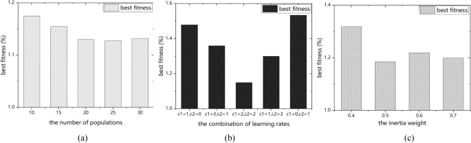
The impact of the factors on best fitness (a), the number of populations (b), the combinations of learning rates (c), and the inertia weight
-
Step 4 Calculate the fitness value of each particle position \(X_{i}\), and calculate the optimal position of the individual particle according to the initial particle fitness value. Then use the current best position of each particle as the initial position to find the global optimum position.
-
Step 5 In each iteration, use the individual and global optimal values to renew the particle velocity and position, and then compute the updated particle’s fitness. If the fitness of the new one is better than that of all previous particles, then update current optimal and the global optimal position [29].
-
Step 6 After reaching the maximum number of iterations, the hyperparameters \(h_{1} ,h_{2} ,n\) of the global optimal position are output and substituted into the original LSTM model for prediction.

4 Case Analysis
In this section, three models were built to predict the passenger flow on the two scenarios of workdays and holidays. First, a basic LSTM model was established using only one set of hyperparameters and parameters. However, subway running hour contains different time periods such as high peak hour and low peak hour, and the regularity and volume of passenger flow in each time period is varied. Different time periods were divided separately in workday and holiday scenarios, and eight LSTM prediction models were established on the basis of different time periods. In the training model process, the hyperparameters were difficult to determine. Therefore, the PSO was used to search the optimal hyperparameters setting in the multisource data LSTM.
To fully validate each prediction model, a SVM model was selected that represents a traditional machine learning model compared with the LSTM basic and LSTM optimized models.
4.1 Evaluation Indexes
To evaluate the prediction accuracy, the following four error indexes were selected: mean square error (MSE), root mean square error (RMSE), mean absolute error (MAE), and mean absolute percentage error (MAPE) [30]. The specific calculations of each error index are shown in Equations (3–6):
\(y_{i}\) is the actual inbound volume of the station at time \(i\). \(\widehat{{y_{i} }}\) is the predicted inbound volume of the station at time \(i\). \(\overline{y}\) is the average actual inbound volume of the station. \(n\) is the number of data in the time series of inbound passenger flow at this station.
The passenger flow on workdays will be large and regular due to the commuter passenger flow in peak hours, while the passenger flow on holidays will be scattered and irregular. Considering the different passenger flow regularity on time dimensions, this study established passenger flow prediction models on workdays and holidays.
4.2 Subway Passenger Flow Prediction in Workday Scenario (A1)
4.2.1 Subway Passenger Flow Prediction on Workdays
-
(1)
Basic LSTM model
For the training process of the LSTM prediction model, two layers of LSTM hidden layers were set. To avoid the high degree of specialization of neuron weights leading to overfitting of the model, two dropout layers were added, and the random inactivation probability of these two layers was set to 0.2 and 0.1, respectively. The ReLU function was selected as the excitation function of the model, and MAE as the loss function [31]. This paper used Adam optimizer, which would customize the initial learning rate to 0.001 and automatically update the learning rate of each parameter in each round through an adaptive method.
According to the empirical knowledge, the hyperparameters of the LSTM prediction model was set on workday scenarios. The number of Epoch iterations was 100, Batch Size iterations was 256, and the number of neurons was 128 and 256 in the first and second LSTM hidden layers, respectively.
-
(2)
LSTM based on different time periods
According to the cluster analysis results in Section 3.1, there are four different time periods (B1, B2, B3, and B4) under the workday scenario (A1). In this section, four LSTM optimized models based on different time periods were built with the same hyperparameters as the basic LSTM model.
-
(3)
PSO-LSTM based on different time periods
The PSO algorithm on the LSTM model based on different time periods was used to further optimize the hyperparameter searching process. The particle swarm parameters were defined: the number of populations was 20, the number of iterations was 15, the learning factor was \(c_{1} = c_{2} = 2\), and the inertia weight was taken as \(w = 0.5\). The parameter value range of particle \(X_{i,0} \left( {h_{1} ,h_{2} ,n} \right)\) was [10,400], [10,400], and [10,200], and the value range of velocity was [−45, 45], [−45, 45], and [−20, 20], respectively. Taking A1B2 as an example, the global optimal parameters of the LSTM model particle swarm were stable at \(h_{1} = 104,\rm{}h_{2} = 279,\rm{}n = 113\) in the A1B2 time period.
Through the PSO algorithm, different combinations of hyperparameters are continuously substituted into the LSTM model for training, and the global optimal hyperparameters are found during continuous adjustments. At this time, the value of the hyperparameters also tend to be stable.
Sensitivity analysis is a method to determine how the change of a state or output of a system or model can influence the whole model. To illustrate the rationality of the input parameter settings of PSO-LSTM, this section performed necessary sensitivity analyses with respect to the input parameters. The main factors that affect the efficiency of PSO algorithm optimization are the number of populations, the learning factor, and the inertia weight. Therefore, as shown in Fig.5, this part will discuss the sensitivity of these three factors in the PSO-LSTM model.
-
(1)
The number of populations
When the number of populations is small the algorithm converges quickly; however, it can easily fall into the local optimum. When the value is large, the algorithm convergence speed is relatively slow, which would lead to a dramatic increase in the calculation time. In addition, when the number of populations increases to a certain level, it would no longer have a significant effect by increasing the number of particles. In this paper, the number of populations was set as 20. Figure 5(a) shows that, as the number of populations increases, the best fitness (MAPE) drops at first and then remains stable after the value equals 20.
-
(2)
The learning rates
The learning rates c1 and c2 have the ability to learn from themselves and other individuals, so that the particles can approach the best position. If the learning rate is small, particles have possibilities to wander away from the target area; while it is large, the particles move swiftly to or even exceed the ideal targeted area. Therefore, the different combinations of c1 and c2 will affect the performance of the PSO algorithm. To analyze the sensitivity of the learning rates, the combination of the learning rates are set at the endpoint: (1) c1 = 4 and c2 = 0; (2) c1 = 3 and c2 = 1; (3) c1 = 1 and c2 = 3; (4) c1 = 0 and c2 = 4. As shown in Fig. 5(b), the bar chart is roughly symmetrical, with poor “best fitness” results near the two endpoints. In addition, it can be seen that the impact of the learning rate change is weaker than the change of the number of populations on the value of best fitness. It can be concluded that the influence of the learning rates on the best fitness is higher than the population size.
-
(3)
The inertia weight
The bigger the value of the inertia weight w, the greater the particle’s flight speed, and the particle will perform a global search with a larger step length; the smaller the value of w, the smaller the particle step, which tends to be a fine local search. To explore the influence of different weights on best fitness, the inertia weight w is selected from 0.4 to 0.7, and gradually increased. The trend of best fitness is shown in Fig. 5(c). It can be seen that, as the inertia weight increases, the best fitness first drops sharply and then slowly rises. When w = 0.5, the best fitness value is the smallest Fig 5.
According to the above sensitivity analysis, the following can be identified:
-
(1)
The increase in the number of populations will result in a small decrease in best fitness, but after increasing to a certain size, it will no longer affect best fitness.
-
(2)
The optimization efficiency is poor when the value of the learning rates is at both ends. In addition, best fitness is more sensitive to learning rates than to the number of populations.
-
(3)
The inertia weight has a greater impact on best fitness. As the inertia weight increases, the best fitness will first decrease and then increase at a slow rate.
4.2.2 Comparison and Analysis between Prediction Models
To compare the prediction performance of each model, the passenger flow prediction curves of each model were plotted in one graph, shown in Fig. 6. The error indexes of each prediction model in the workday scenario are presented in Table 2.

True and predicted passenger flow in a workday in 2018
The outcome of the prediction LSTM model conformed to the characteristics of original passenger flow on workdays, and the tide phenomenon appeared in the morning and evening. The predicted value fitted the true value well and the goodness of fit reached 0.986, which proved that the LSTM model can learn the changing regularity of passenger flow data. During workdays, due to the existence of morning and evening peaks, the upward and downward trends of passenger flow are more obvious, which is conducive to the LSTM model to learn the changes of passenger flow.
Comparing the performance of SVR and LSTM in short-term subway passenger flow prediction, the prediction performance of the LSTM model is better than that of the SVR model, with a MAPE of 21.97% in the LTSM model, which is lower than that of the SVR model. According to the predicted passenger flow graphs, it can be seen that the passenger flow trend of the SVR workday model conforms to the actual passenger flow change regularity, but the prediction accuracy is not high in each time interval. While the LSTM model shows that the fitting effect is accurate at off-peak periods in the workday scenario, and the error mostly occurs during peak hours with large passenger flow.
The basic and optimized LSTM models have reached a good overall prediction effect, but there are some prediction results that deviate from the true value. The two optimized models have improved prediction performances compared with the basic LSTM model. The LSTM model based on different time periods has considered the variance of passenger flow from different time periods. The PSO-LSTM optimization effect is better, with MAPE of up to 3.63%, which is lower than that of the LSTM model based on different time periods. This improves the optimization effect by searching the best hyperparameter combination at the cost of time.
4.3 Subway Passenger Flow Prediction in Holiday Scenario (A2)
4.3.1 Subway Passenger Flow Prediction on Holidays
The model structure of the LSTM in the holiday scenario is the same as that of workday, but the hyperparameters are different. The number of Epoch iterations is 50 and Batch Size is 256, and the number of neurons in the first and second LSTM hidden layers were 24 and 48, respectively.
The change trend of passenger flow was in line with the overall passenger flow trend and the goodness of fit was 0.965, which showed a good fit. However, at certain moments when the passenger flow changed drastically, the prediction effect was poor, with an error of more than 100 people from the true data.
As for the validations of optimized models in the holiday scenario, the optimization model experiment process in the holiday scenario is consistent with the optimization prediction model in the working day scenario in Section 4.2.1, and the hyperparameters of the LSTM model based on different time periods are as the same as those of the basic LSTM model of a holiday scenario
4.3.2 Comparison and Analysis between Prediction Models
The prediction passenger flow curve graph is shown in Fig. 7. The error indexes of each prediction model in the holiday scenario are presented in Table 3.

True and predicted passenger flow in a holiday in 2018
The MSE, RMSE, and MAE of the SVR model are slightly smaller than the LSTM model in the holiday scenario, indicating that its dispersion is smaller and the deviation between the predicted value and the true value is less. This shows that there are many outliers in the prediction of the LSTM model. The MAPE of LSTM is lower than that of SVR. The MAPE of LSTM model is 13.89%, while the MAPE of SVR is 18.69%, showing that the prediction of LSTM is better than SVR on holidays.
Comparing the prediction models in the holiday scenario, optimized models have higher prediction accuracy than the basic LSTM model. In the case of LSTM based on different time periods, MAPE was sharply reduced to 4.16%, and the MAPE of PSO-LSTM based on different time periods reached 3.00%.
5 Conclusions
-
(1)
In this study, we collected original AFC data in two months of 2018 and processed them according to the cleansing rules. The cleansed data in2018 amounted to 5,975,136 trips in 2 months (1 April to 31 May), of which the data in April accounted for 2,944,086 and the data in May were 3,031,050 trips.
-
(2)
Since deep learning has strong adaptability and it is easy to construct feature vectors, this paper chose the LSTM method was chosen to build a short-term subway passenger flow prediction model. Aiming at overcoming the shortcomings found in the verification process of the LSTM prediction model, optimizations were made gradually. First, for the errors that mostly occur during peak hours with a high volume of passenger flow, the LSTM based on different time periods was proposed to make corresponding passenger flow predictions at various time periods. After that, the PSO algorithm was used to search for the optimal hyperparameter settings in previously optimized models. The effectiveness of basic and optimized LSTM models was verified in two scenarios as workdays and holidays. Then the prediction results were compared with the traditional machine learning SVR model. The results showed that the overall prediction performance of the SVR model was worse than that of LSTM, with MAPE on workdays and holidays of 21.97% and 4.80%, respectively, lower than that of the LSTM, which verified that the LSTM-based model’s predictive performance was superior to traditional machine learning SVR in both scenarios.
-
(3)
The LSTM model based on different time periods has a certain optimization effect after dividing the subway running hours into four different time periods. The prediction error MAPE of the LSTM model based on different time periods on workday and holiday scenarios was 5.50% and 4.16%, respectively, lower than the MAPE of the basic LSTM model on workdays (12.48%) and holidays (13.89%). The PSO-LSTM model searches for a set of model hyperparameters with higher prediction accuracy at the expense of running time. The prediction error of the PSO-LSTM dropped by 1.87% and 1.16% in each scenario compared with the model without PSO algorithm.
-
(4)
The optimized models can improve the accuracy of short-term subway passenger flow prediction. A more accurate prediction of passenger flow brings convenience to the operational plans of the subway company. According to the variances of passenger flow in different scenarios, corresponding train operation plans can be formulated. In addition, passenger flow evacuation plans can be made in advance according to the peak passenger flow, to reduce the possibility of accidents.
-
(5)
In future research, the speed of PSO optimization for searching hyperparameters still needs improving. In this study, the scope of the research focused on only one station, which could be expanded to the whole subway line to consider the interaction between stations to generate the prediction.
References
He J (2013) Urban Railway traffic passenger flow statistical characteristics analysis and empirical study on the combination forecast method. Beijing Jiaotong University, Beijing
Zhao J, Gao Y, Yang Z, Li J, Feng Y, Qin Z, Bai Z (2019) Truck traffic speed prediction under non-recurrent congestion: Based on optimized deep learning algorithms and GPS Data. IEEE Access 7(1):9116–9127. https://doi.org/10.1109/ACCESS.2018.2890414
Wang X (2018) Study on accessibility of urban public transit based on smart card data. Beijing Jiaotong University, Beijing
Zhao J, Shi J, Sun Q, Ren L, Liu C (2020) Short-time Inflow and outflow prediction of metro stations based on hybrid deep learning. J Transp Syst Eng Inf Technol 20(5):128–134. https://doi.org/10.16097/j.cnki.1009-6744.2020.05.019.(inChinese)
Hou C, Sun H, Zhou Y, Cao B, Fan J (2019) Prediction service of subway short-term passenger flow based on neural network. Journal of Chinese Computer Systems 40(1):226–231. https://doi.org/10.3969/j.issn.1000-1220.2019.01.041.(inChinese)
Hamed MM, Al-masaeid HR, Bani S, Zahi M (1995) Short-term prediction of traffic volume in urban arterials[J]. J Transp Eng 121(3):249–254. https://doi.org/10.1061/(ASCE)0733-947X(1995)121:3(249)
Wang Y, Han B, Zhang Q, Li D (2015) Forecasting of entering passenger flow volume in Beijing subway based on SARIMA model. J Transp Syst Eng Inf Technol 15(6):205–211. https://doi.org/10.3969/j.issn.1009-6744.2015.06.031.(inChinese)
GirakaI O, Selvaraj VK (2020) Short-term prediction of intersection turning volume using seasonal ARIMA model. Transp Lett 12(7):483–490. https://doi.org/10.1080/19427867.2019.1645476
Cui H, Chen X, Yang C, Xiang Y, Duan H (2019) Forecast of subway inbound passenger flow based on DLSTM recurrent network. Urban Mass Transit 22(09):41–45. https://doi.org/10.16037/j.1007-869x.2019.09.009.(inChinese)
Liu Y, Liu Z, Jia R (2019) DeepPF: A deep learning based architecture for metro passenger flow prediction. Transp Res Part C: Emerg Technol 101:18–34. https://doi.org/10.1016/j.trc.2019.01.027
Ding A, Zhao X, Jiao L (2002). Traffic flow time series prediction based on statistics learning theory. IEEE 5th International Conference on Intelligent Transportation Systems. Inst Electric Electron Eng Inc, pp. 727–730. DOI: https://doi.org/10.1109/ITSC.2002.1041308
Bai Y, Sun Z, Zeng B, Deng J, Li C (2017) A multi-pattern deep fusion model for short-term bus passenger flow forecasting. Appl Soft Comput J 58:669–680. https://doi.org/10.1016/j.asoc.2017.05.011
Hao S, Lee D, Zhao D (2019) Sequence to sequence learning with attention mechanism for short-term passenger flow prediction in large-scale metro system. Transp Res Part C: Emerg Technol 107:287–300. https://doi.org/10.1016/j.trc.2019.08.005
Tsai T, Lee C, Wei C (2009) Neural network based temporal feature models for short-term railway passenger demand forecasting. Exp Syst Appl 36(2):3728–3736
Yang J, Zhu J, Liu B, Feng C, Zhang H (2019) Short-term passenger flow prediction for urban railway transit based on combined mode. J Transp Syst Eng Inf Technol 19(3):119–125. https://doi.org/10.16097/j.cnki.1009-6744.2019.03.018.(inChinese)
Liu Y, Zou B, Ni A, Gao L, Zhang C (2021) Calibrating microscopic traffic simulators using machine learning and particle swarm optimization. Transp Lett 13(4):295–307. https://doi.org/10.1080/19427867.2020.1728037
Zhao J, Wang X (2019) Vehicle-logo recognition based on modified HU invariant moments and SVM. Multimed Tools Appl 78(1):75–97. https://doi.org/10.1007/s11042-017-5254-0
Lin L, He Z, Peeta S (2018) Predicting station-level hourly demand in a large-scale bike-sharing network: A graph convolutional neural network approach. Transp Res Part C Emerg Technol 97:258–276. https://doi.org/10.1016/j.trc.2018.10.011
Du B, Peng H, Wang S, Bhuiyan MZA, Wang L, Gong Q, Liu L, Li J (2020) Deep irregular convolutional residual LSTM for urban traffic passenger flows prediction. IEEE Trans Intell Transp Syst 21(3):972–985. https://doi.org/10.1109/TITS.2019.2900481
Lv Y, Duan Y, Kang W, Li Z, Wang F (2015) Traffic flow prediction with big data: A deep learning approach. IEEE Trans Intell Transp Syst 16(2):865–873. https://doi.org/10.1109/TITS.2014.2345663
Du Y (2015) The research and implementation of Beijing subway passenger flow prediction system. Beijing Jiaotong University, Beijing
Sha S, Li J, Zhang K, Yang Z, Wei LX, Zhu X (2020) RNN-Based subway passenger flow rolling prediction. IEEE ACCESS 8:15232–15240. https://doi.org/10.1109/ACCESS.2020.2964680
Zhao J, Gao Y, Bai Z, Wang H, Lu S (2019) Traffic speed prediction under non-recurrent congestion: Based on LSTM method and beidou navigation satellite system data. IEEE Intell Transp Syst Mag 11(2):70–81. https://doi.org/10.1109/MITS.2019.2903431
Li M, Li J, Wei Z, Wang S, Chen L (2018) Short-time passenger flow forecasting at subway station based on deep learning LSTM structure. Urban Mass Trans 21(11):42–49
Li W, Feng F, Jiang Q (2018) Prediction for railway passenger volume based on modified PSO optimized LSTM neural network. J Railway Sci Eng 15(12):3274–3280. https://doi.org/10.19713/j.cnki.43-1423/u.2018.12.033.(inChinese)
Zhao J, Gao Y, Guo Y, Bai Z (2018) Travel time prediction of expressway based on multi-dimensional data and the particle swarm optimization–autoregressive moving average with exogenous input model. Adv Mech Eng 10(2):1–16. https://doi.org/10.1177/1687814018760932
Long X, Li J, Chen Y (2019) Metro short-term traffic flow prediction with deep learning. Control and Decision 34(08):1589–1600. https://doi.org/10.13195/j.kzyjc.2018.1393.(inChinese)
Wang X (2017) Research on short-term passenger flow forecast of urban rail transit line. Beijing Jiaotong University, Beijing
Qin Y (2019) Short-term passenger flow forecast of urban rail transit stations based on AFC data. Beijing Jiaotong University, Beijing
Zhao Y, Xia L, Jiang X (2020) Short-term metro passenger flow prediction based on EMD-LSTM. J Traffic and Trans Eng 20(04):194–204. https://doi.org/10.19818/j.cnki.1671-1637.2020.04.016.(inChinese)
Liang D, Xu J, Li S, Sun C (2020) Short-term passenger flow prediction of rail transit based on VMD-LSTM neural network combination model. Proceedings of the 32nd Chinese Control and Decision Conference, CCDC 2020, Institute of Electrical and Electronics Engineers Inc, pp. 5131-5136. DOI: https://doi.org/10.1109/CCDC49329.2020.9164470
Funding
This work is supported by the National Key Research and Development Program of China (No. 2019YFB1600200), National Natural Science Foundation of China (71871011, 71890972/71890970, 71621001).
Author information
Authors and Affiliations
Contributions
The authors confirm contribution to the paper as follows: conceptualization: JZ, RJ, JL; formal analysis: JL, DZ; data collection: JZ, DZ; methodology: JL, DZ; validation and visualization: JL; writing-original paper: JL; writing-review and editing: DZ, JZ; supervision: RJ, JZ; funding acquisition: RJ, JZ.
Corresponding author
Ethics declarations
Conflict of interest
The authors declare that they have no known competing financial interests or personal relationships that could have appeared to influence the work reported in this pap
Additional information
Communicated by Baoming Han.
Rights and permissions
Open Access This article is licensed under a Creative Commons Attribution 4.0 International License, which permits use, sharing, adaptation, distribution and reproduction in any medium or format, as long as you give appropriate credit to the original author(s) and the source, provide a link to the Creative Commons licence, and indicate if changes were made. The images or other third party material in this article are included in the article's Creative Commons licence, unless indicated otherwise in a credit line to the material. If material is not included in the article's Creative Commons licence and your intended use is not permitted by statutory regulation or exceeds the permitted use, you will need to obtain permission directly from the copyright holder. To view a copy of this licence, visit http://creativecommons.org/licenses/by/4.0/.
About this article

Cite this article
Liu, J., Jiang, R., Zhu, D. et al. Short-Term Subway Inbound Passenger Flow Prediction Based on AFC Data and PSO-LSTM Optimized Model. Urban Rail Transit 8, 56–66 (2022). https://doi.org/10.1007/s40864-022-00166-x
Received:
Revised:
Accepted:
Published:
Issue Date:
DOI: https://doi.org/10.1007/s40864-022-00166-x