


1 Introduction
This paper is roughly divided into two parts. In Section 1 we state our main technical results on point counting for foliations. This includes upper bounds for the number of intersections between a leaf of a foliation and an algebraic variety (Theorem 1), a corresponding bound for the covering of such intersections by Weierstrass polydiscs (Theorem 2) and consequently a counting result for algebraic points in terms of height and degree (Theorem 3) in the spirit of the Pila–Wilkie theorem and Wilkie’s conjecture. The proofs of these result are given in Sections 2–6.
In the second part, starting with Section 7, we state three applications of our point-counting results in Diophantine geometry. These include an effective form of Masser–Zannier bound for simultaneous torsions points on squares of elliptic curves, and in particular effective polynomial-time computability of this set; a polynomial bound for Pila’s proof of the André–Oort conjecture for  ${\mathbb C}^{n}$, and in particular the polynomial-time decidability (by an algorithm with an ineffective constant); and a proof of Galois-orbit lower bounds for torsion points in elliptic curves following an idea of Schmidt. We also briefly describe the results of [Reference Binyamini, Schmidt and Yafaev15] (joint with Schmidt and Yafaev), which uses a similar strategy to prove Galois-orbit lower bounds for special points in Shimura varieties. The proofs of these results are given in Sections 8–10.
Finally, in Appendix A we prove some growth estimates for solutions of inhomogeneous Fuchsian differential equations over number fields. These are used in our treatment of the Masser–Zannier result and would probably be similarly useful in many of its generalisations.
1.1 Setup
In this section we introduce the main notations and terminology used throughout the paper.
1.1.1 The variety
Let  ${\mathbb M}\subset {\mathbb A}^{N}_{\mathbb K}$ be an irreducible affine variety defined over a number field
  ${\mathbb K}$. We equip
  ${\mathbb M}$ with the standard Euclidean metric from
  ${\mathbb A}^{N}$, denoted ‘
 $\operatorname {dist}$’, and denote by
  ${\mathbb B}_{R}\subset {\mathbb M}$ the intersection of
  ${\mathbb M}$ with the ball of radius R around the origin in
  ${\mathbb A}^{N}$. Set
  ${\mathbb B}:=B_{1}$.
1.1.2 The foliation
Let  ${\boldsymbol \xi }:=(\xi _{1},\dotsc ,\xi _{n})$ denote n commuting, generically linearly independent, rational vector fields on
  ${\mathbb M}$ defined over
  ${\mathbb K}$. We denote by
  ${\mathcal F}$ the (singular) foliation of
  ${\mathbb M}$ generated by
  ${\boldsymbol \xi }$ and by
  $\Sigma _{\mathcal F}\subset {\mathbb M}$ the union of the polar loci of
  $\xi _{1},\dotsc ,\xi _{n}$ and the set of points where they are linearly dependent.
For every  $p\in {\mathbb M}\setminus \Sigma _{\mathcal F}$, denote by
  ${\mathcal L}_{p}$ the germ of the leaf of
  ${\mathcal F}$ through p. We have a germ of a holomorphic map
  $\phi _{p}:({\mathbb C}^{n},0)\to {\mathcal L}_{p}$ satisfying
  $\partial \phi _{p}/\partial x_{i}=\xi _{i}$ for
  $i=1,\dotsc ,n$. We refer to this coordinate chart as the
  ${\boldsymbol \xi }$-coordinates on
  ${\mathcal L}_{p}$.
1.1.3 Balls and polydiscs
If  $A\subset {\mathbb C}^{n}$ is a ball (resp., polydisc) and
  $\delta>0$, we denote by
  $A^{\delta }$ the ball (resp., polydisc) with the same centre where the radius r (resp., each radius r) is replaced by
  $\delta ^{-1}r$. If
  $\phi _{p}$ continues holomorphically to a ball
  $B\subset {\mathbb C}^{n}$ around the origin, then we call
  ${\mathcal B}:=\phi _{p}(B)$ a
  ${\boldsymbol \xi }$-ball. If
  $\phi _{p}$ extends to
  $B^{\delta }$, we denote
  ${\mathcal B}^{\delta }:=\phi _{p}\left (B^{\delta }\right )$.
1.1.4 Degrees and heights
We denote by  $h:{\mathbb Q}^{\mathrm {alg}}\to {\mathbb R}_{\ge 0}$ the absolute logarithmic Weil height. If
  $x\in {\mathbb Q}^{\mathrm {alg}}$ has minimal polynomial
  $a_{0}\prod _{i=1}^{d}(x-x_{i})$ over
  ${\mathbb Z}[x]$, then
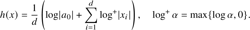 $$ \begin{align} h(x) = \frac1d\left(\log \lvert a_{0}\rvert + \sum_{i=1}^{d} \log^{+}\lvert x_{i}\rvert\right), \quad \log^{+}\alpha=\max\{\log\alpha,0\}. \end{align} $$
We also denote  $H(x):=e^{h(x)}$. We define the height of a vector
  ${\mathbf x}\in \left ({\mathbb Q}^{\mathrm {alg}}\right )^{n}$ as the maximal height of the coordinates.
For a polynomial P, we set  $\delta (P):=\max (\deg P,h(P))$, where h(P) denotes the logarithmic height of the polynomial P. For a variety
  $V\subset {\mathbb M}$, we denote by
  $\deg V$ the degree with respect to the standard projective embedding
  ${\mathbb A}^{n}\to {\mathbb P}^{n}$; we define
  $h(V)$ as the height of the Chow coordinates of V with respect to this embedding. For a vector field
  ${\boldsymbol \xi }$, we define
  $\deg {\boldsymbol \xi }$ (resp.,
  $h({\boldsymbol \xi })$) as the maximum degree (resp., logarithmic height) of the polynomials
  ${\boldsymbol \xi }({\mathbf x}_{i})$, where
  ${\mathbf x}_{i}$ are the affine coordinates on the ambient space. Finally we set
 $$ \begin{align} \delta_{\mathbb M}:=\max([{\mathbb K}:{\mathbb Q}],\deg{\mathbb M},h({\mathbb M})) \end{align} $$
and
 $$ \begin{align} \delta(V) := \max(\delta_{\mathbb M},\deg V,h(V)), \qquad \delta({\boldsymbol\xi}):=\max(\delta_{\mathbb M},\deg{\boldsymbol\xi},h({\boldsymbol\xi})). \end{align} $$
We sometimes write  $\delta _{P},\delta _{V},\delta _{\boldsymbol \xi }$ for
  $\delta (P),\delta (V),\delta ({\boldsymbol \xi })$, to avoid cluttering the notation.
1.1.5 The unlikely intersection locus
Let  $V\subset {\mathbb M}$ be a pure-dimensional subvariety of codimension at most n defined over
  ${\mathbb K}$. We define the unlikely intersection locus of V and
  ${\mathcal F}$ to be
 $$ \begin{align} \Sigma_{V} := \Sigma_{\mathcal F}\cup\left\{ p\in{\mathbb M}: \dim\left(V\cap{\mathcal L}_{p}\right)>n-\operatorname{codim} V\right\}, \end{align} $$
that is, the set of points p where V intersects  ${\mathcal L}_{p}$ improperly.
1.1.6 Weierstrass polydiscs
Let  ${\mathcal B}$ be a
  ${\boldsymbol \xi }$-ball. We say that a coordinate system
  ${\mathbf x}$ is a unitary coordinate system if it is obtained from the
  ${\boldsymbol \xi }$-coordinates by a linear unitary transformation.
Let  $X\subset {\mathcal B}$ be an analytic subset of pure dimension m. We say that a polydisc
  $\Delta :=\Delta _{z}\times \Delta _{w}$ in the unitary
  ${\mathbf x}={\mathbf z}\times {\mathbf w}$-coordinates is a Weierstrass polydisc for X if
  $\bar \Delta \subset {\mathcal B}$ and if
  $\dim \Delta _{z}=m$ and
  $X\cap \left (\bar \Delta _{z}\times \partial \Delta _{w}\right )=\emptyset $. In this case, the projection
  $\Delta \cap X\to \Delta _{z}$ is a proper ramified covering map, and we denote its (finite) degree by
  $e(\Delta ,X)$ and call it the degree of X in
  $\Delta $.
1.1.7 Asymptotic notation
We use the asymptotic notation  $Z=\operatorname {poly}_{X}(Y)$ to mean that
  $Z<P_{X}(Y)$, where
  $P_{X}$ is a polynomial depending on X. In this text the coefficients of
  $P_{X}$ can always be explicitly computed from X unless explicitly stated otherwise. We similarly write
  $Z=O_{X}(Y)$ for
  $Z< C_{X}\cdot Y$, where
  $C_{X}\in {\mathbb R}_{\ge }0$ is a constant depending on X.
Throughout the paper, the implicit constants in asymptotic notation are assumed to depend on the ambient dimension of  ${\mathbb M}$, which we omit for brevity. All implicit constants are effective unless explicitly stated otherwise (this occurs only in Theorem 7 on the André–Oort conjecture for powers of the mdoular curve).
1.2 Statement of the main results
Our first main theorem is the following bound for the number of intersections between a  ${\boldsymbol \xi }$-ball and an algebraic variety of complementary dimension. Throughout this section, we let R denote a positive real number.
Theorem 1. Suppose  $\operatorname {codim} V=n$ and let
  ${\mathcal B}\subset {\mathbb B}_{R}$ be a
  ${\boldsymbol \xi }$-ball of radius at most R. Then
 $$ \begin{align} \#\left({\mathcal B}^{2}\cap V\right) = \operatorname{poly}\left(\delta_{\boldsymbol\xi},\delta_{V},\log R,\log\operatorname{dist}^{-1}({\mathcal B},\Sigma_{V})\right), \end{align} $$
where intersection points are counted with multiplicities.
The reader may for simplicity consider the case  $R=1$. The general case reduces to this case immediately by rescaling the coordinates on
  ${\mathbb M}$ and the vector fields
  $\xi $ by a factor of R. This rescaling factor enters logarithmically into
  $\delta _{V}$ and
  $\delta _{\boldsymbol \xi }$, hence the dependence on
  $\log R$ in the general case. To simplify our presentation, we will therefore consider only the case
  $R=1$ in the proof of Theorem 1.
Remark 1. Similar to the comment just made, by rescaling each coordinate separately we may also work with arbitrary polydiscs instead of arbitrary balls.
We also record a corollary which is sometimes useful in the case of higher codimensions:
Corollary 2. Let  $V\subset {\mathbb M}$ have arbitrary codimension and set
 $$ \begin{align} \Sigma := \Sigma_{\mathcal F} \cup\left\{ p\in{\mathbb M}: \dim\left(V\cap{\mathcal L}_{p}\right)>0\right\}. \end{align} $$
Let  ${\mathcal B}\subset {\mathbb B}_{R}$ be a
  ${\boldsymbol \xi }$-ball of radius at most R. Then
 $$ \begin{align} \#\left({\mathcal B}^{2}\cap V\right) = \operatorname{poly}\left(\delta_{\boldsymbol\xi},\delta_{V},\log R,\log\operatorname{dist}^{-1}({\mathcal B},\Sigma)\right), \end{align} $$
where intersection points are counted with multiplicities.
Our second main theorem states that the intersection between a  ${\boldsymbol \xi }$-ball and a subvariety admits a covering by Weierstrass polydiscs of effectively bounded size:
Theorem 2. Suppose  $\operatorname {codim} V\le n$ and let
  ${\mathcal B}\subset {\mathbb B}_{R}$ be a
  ${\boldsymbol \xi }$-ball of radius at most R. Then there exists a collection of Weierstrass polydiscs
  $\{\Delta _{\alpha }\subset {\mathcal B}\}$ for
  ${\mathcal B}\cap V$ such that the union of
  $\Delta ^{2}_{\alpha }$ covers
  ${\mathcal B}^{2}$ and
 $$ \begin{align} \#\{\Delta_{\alpha}\},\max_{\alpha} e({\mathcal B}\cap V,\Delta_{\alpha}) = \operatorname{poly}\left(\delta_{\boldsymbol\xi},\delta_{V},\log R,\log\operatorname{dist}^{-1}({\mathcal B},\Sigma_{V})\right). \end{align} $$
 The same comment on rescaling to the case  $R=1$ applies to this theorem as well.
Remark 3. It would also have been possible to state our results in invariant language for a general algebraic variety and its foliation without fixing an affine chart and a basis of commuting vector fields. We opted for the less-invariant language in order to give an explicit description of the dependence of our constants on the foliation  ${\mathcal F}$ and the relatively compact domain
  ${\mathcal B}\subset {\mathcal F}$ being considered.
1.3 Counting algebraic points
For this section we fix  $\ell \in {\mathbb N}$, a map
  $\Phi \in {\mathcal O}({\mathbb M})^{\ell }$ defined over
  ${\mathbb K}$, an algebraic
  ${\mathbb K}$-variety
  $V\subset {\mathbb M}$ and a
  ${\boldsymbol \xi }$-ball
  ${\mathcal B}\subset {\mathbb B}_{R}$ of radius at most R. Set
 $$ \begin{align} A = A_{V,\Phi,{\mathcal B}} := \Phi\left({\mathcal B}^{2}\cap V\right) \subset {\mathbb C}^{\ell}. \end{align} $$
Denote
 $$ \begin{align} A(g,h) := \{ p\in A : [{\mathbb Q}(p):{\mathbb Q}] \le g \text{ and } h(p)\le h\}. \end{align} $$
Our goal will be to study the sets  $A(g,h)$ in the spirit of the Pila–Wilkie counting theorem [Reference Pila and Wilkie47]. Toward this end, we introduce the following notation:
Definition 4. Let  ${\mathcal W}\subset {\mathbb C}^{\ell }$ be an irreducible algebraic variety. We denote by
  $\Sigma (V,{\mathcal W};\Phi )$ the union of (i) the points p where the germ
  $\Phi {\vert _{{\mathcal L}_{p}\cap V}}$ is not a finite map and (ii) the points p where
  $\Phi \left ({\mathcal L}_{p}\cap V\right )$ contains one of the analytic components of the germ
  ${\mathcal W}_{\Phi (p)}$. We omit
  $\Phi $ from the notation if it is clear from the context.
In most applications,  $\Phi $ will be a set of coordinates on the leaves of our foliation and condition (i) will be empty. Condition (ii) then states that
  $\Phi \left ({\mathcal L}_{p}\cap V\right )$ contains a connected semialgebraic set of positive dimension (namely a component of
  ${\mathcal W}$). Our main result is the following:
Theorem 3. Set  $\varepsilon>0$. There exists a collection of irreducible
  ${\mathbb Q}$-subvarieties
  $\left \{{\mathcal W}_{\alpha }\subset {\mathbb C}^{\ell }\right \}$ such that
  $\operatorname {dist}({\mathcal B},\Sigma (V,{\mathcal W}_{\alpha }))<\varepsilon $,
 $$ \begin{align} A(g,h) \subset \cup_{\alpha} {\mathcal W}_{\alpha} \end{align} $$
and
 $$ \begin{align} \#\{{\mathcal W}_{\alpha}\}, \max_{\alpha} \delta_{{\mathcal W}_{\alpha}} = \operatorname{poly}\left(\delta_{\boldsymbol\xi},\delta_{V},\delta_{\Phi},g,h,\log R,\log \varepsilon^{-1}\right). \end{align} $$
 As with Theorem 1, one can always reduce to the case  $R=1$ in this theorem by rescaling, and we will consider only the case
  $R=1$ in the proof.
Remark 5 blocks from nearby leaves
Theorem 3 can be viewed as an analogue of the Pila–Wilkie theorem in its blocks formulation [Reference Pila44]. Suppose for simplicity that  $\Phi $ is such that condition (i) in Definition 4 is automatically satisfied for all leaves. The
  $\{{\mathcal W}_{\alpha }\}$ are similar to blocks in the sense that they are algebraic varieties containing all of
  $A(g,h)$. The difference is that in the Pila–Wilkie theorem, these blocks are all subsets of
  $A^{\mathrm {alg}}$. In Theorem 3 one should think of the set A as belonging to a family
  $A_{\mathcal L}$, parametrised by varying the leaf
  ${\mathcal L}$ while keeping
  $V,\Phi $ fixed. The blocks
  ${\mathcal W}_{\alpha }$ correspond to some algebraic part, but possibly of an
  $A_{\mathcal L}$ for a nearby leaf
  ${\mathcal L}$ (at distance
  $\varepsilon $ from the original leaf). We therefore refer to
  $\{W_{\alpha }\}$ as blocks coming from nearby leaves.
Ideally one would hope to obtain a result with equation (12) independent of  $\varepsilon $, which would eliminate the need to consider blocks from nearby leaves and give a result roughly analogous to a block-counting version of the Wilkie conjecture. Unfortunately, due to the dependence in our main theorems on
  $\log \operatorname {dist}^{-1}({\mathcal B},\Sigma _{V})$, we cannot expect to derive such a result. On the other hand, in practical applications of the counting theorem one usually has good control over the possible blocks, not only on
  ${\mathcal B}$ but on all nearby leaves. We briefly comment on the mechanism that allows this control.
The foliations normally used in Diophantine applications of the Pila–Wilkie theorem are highly symmetric, usually arising as flat structures associated to a principal G-bundle for some algebraic group G. This implies that the nearby leaves are obtained as symmetric images (by a symmetry  $\varepsilon $-close to the identity) of the given leaf. To apply Theorem 3, one describes a transcendental set of interest in the form A already given, where
  ${\mathcal L}$ is taken to be some specific leaf of a foliation. If the classical Pila–Wilkie theorem is applicable, one must already have a description of the algebraic part
  $A^{\mathrm {alg}}$ – usually as a consequence of some functional transcendence statement. When the nearby leaves are obtained from
  ${\mathcal L}$ by some algebraic transformation, this usually implies that one also understands the algebraic blocks coming from these nearby leaves. Theorem 3 then gives an effective polylogarithmic version of the Pila–Wilkie counting theorem, which usually leads to refined information for the Diophantine application. We give several examples of this in Section 7.
As a simple example of this type, we have the following consequence of Theorem 3, in the case where no blocks appear on any of the leaves:
Corollary 6. Suppose that for every  $p\in {\mathbb M}$ the germ
  $\Phi {\vert _{{\mathcal L}_{p}\cap V}}$ is a finite map, and
  $\Phi \left ({\mathcal L}_{p}\cap V\right )$ contains no germs of algebraic curves. Then
 $$ \begin{align} \#A(g,h) = \operatorname{poly}_{\ell}\left(\delta_{\boldsymbol\xi},\delta_{V},\delta_{\Phi},\log R,g,h\right). \end{align} $$
1.4 A result for restricted elementary functions
Recall that the structure of restricted elementary functions is defined by
 $$ \begin{align} {\mathbb R}^{\mathrm{RE}} = \left({\mathbb R},<,+,\cdot,\exp{\vert_{\left[0,1\right]}},\sin{\vert_{\left[0,\pi\right]}}\right). \end{align} $$
 For a set  $A\subset {\mathbb R}^{m}$, we define the algebraic part
  $A^{\mathrm {alg}}$ of A to be the union of all connected semialgebraic subsets of A of positive dimension. We define the transcendental part
  $A^{\mathrm {trans}}$ of A to be
  $A\setminus A^{\mathrm {alg}}$.
In [Reference Binyamini and Novikov12], together with Novikov we established the Wilkie conjecture for  ${\mathbb R}^{\mathrm {RE}}$-definable sets. Namely, according to [Reference Binyamini and Novikov12, Theorem 2], if
  $A\subset {\mathbb R}^{m}$ is
  ${\mathbb R}^{\mathrm {RE}}$-definable then
  $\#A^{\mathrm {trans}}(g,h)=\operatorname {poly}_{A,g}(h)$. Replacing the application of [Reference Binyamini and Novikov12, Proposition 12] with the stronger Proposition 28 established in the present paper yields sharp dependence on g.
Theorem 4. Let  $A\subset {\mathbb R}^{m}$ be
  ${\mathbb R}^{\mathrm {RE}}$-definable. Then
 $$ \begin{align} \#A^{\mathrm{trans}}(g,h) = \operatorname{poly}_{A}(g,h). \end{align} $$
We remark that the proofs of Proposition 28 and consequently Theorem 4 are self-contained and independent of the main technical material developed in this paper. Still, we thought Theorem 4 worth stating explicitly for its own sake, and for putting Theorem 3 into proper context.
1.5 Comparison with other effective counting results
For restricted elementary functions, the approach developed in [Reference Binyamini and Novikov12] gives results that are strictly stronger than the results obtained in this paper – in the sense that the bounds obtained there do not depend on the heights of coefficients or on the distance to the unlikely intersection locus. This can also be generalised to holomorphic-Pfaffian functions, including elliptic and abelian functions. The main limitation of this approach is that it does not seem to apply to period integrals and other maps that arise in problems related to variation of Hodge structures. It therefore does not seem to give an approach for effectivising the main Diophantine applications considered in Theorems 6 and 7. It does apply in the context considered in Theorem 8, but not in the corresponding analogue for Shimura varieties briefly discussed in Section 10.2.
An alternative approach based on the theory of Noetherian functions has been developed in [Reference Binyamini7]. This class does include period integrals and related maps. The results of the present paper have four main advantages:
1. The asymptotic bounds in Theorem 3 depend polynomially on
 $g,h$, whereas the results of [Reference Binyamini7] are for fixed g and subexponential $e^{\varepsilon h}$ in h.
2. The asymptotic bounds in Theorem 3 depend polynomially on the degrees of the equations, whereas in [Reference Binyamini7] the dependence is repeated-exponential. The sharper dependence allows us to obtain the natural asymptotic estimates in the Diophantine applications, leading for instance to polynomial-time algorithms.
3. The results of [Reference Binyamini7] deal strictly with semi-Noetherian sets – that is, sets defined by means of equalities and inequalities but no projections. Theorem 3, on the other hand, allows images under algebraic maps. In many cases, for instance in the proof of Theorem 6, the use of projections is essential and it is difficult, if not impossible, to use [Reference Binyamini7] directly.
4. Both the present paper and [Reference Binyamini7] count points only in compact domains. However, estimates in [Reference Binyamini7] grow polynomially with the radius R of a ball containing the domain, whereas in the present paper they grow polylogarithmically. In many applications this sharper asymptotic allows us to deal with noncompact domains by restricting to sufficiently large compact subsets.


On the other hand, the approach of [Reference Binyamini7] has one main advantage: it gives bounds independent of the log-heights of the equations and the distance to the unlikely intersection locus. Unfortunately, the technical tools used in [Reference Binyamini7] to achieve this are of a very different nature, and we currently do not see a way to combine these approaches. This seems to be a fundamental difficulty related to Gabrielov and Khovanskii’s conjecture on effective bounds for systems of Noetherian equations [Reference Gabrielov and Khovanskii26, Conjectures 1 and 2], which is formulated in the local case and is still open even in this context (but see [Reference Binyamini and Novikov9] for a solution under a mild condition).
1.6 Sketch of the proof
In [Reference Binyamini and Novikov12], the notion of Weierstrass polydiscs was introduced for the purpose of studying rational points on analytic sets. The sets under consideration there are Pfaffian, and an analogu of Theorem 1 (with bounds depending only on  $\deg V$) was already available due to Khovanskii’s theory of fewnomials [Reference Khovanskiĭ32]. One of the main results of [Reference Binyamini and Novikov12] was a corresponding analogue of Theorem 2, established by combining Khovanskii’s estimates with some ideas related to metric entropy.
In the context of arbitrary foliations there is no known analogue for Khovanskii’s theory of fewnomials. It was therefore reasonable to expect that the first step toward generalising the results of [Reference Binyamini and Novikov12] would be to establish such a result on counting intersections, following which one could hopefully deduce a result on covering by Weierstrass polydiscs using a similar reduction. Surprisingly, our proof does not follow this line. Instead, we prove Theorems 1 and 2 by simultaneous induction, using crucially the Weierstrass polydisc construction in dimension  $n-1$ when proving the bound on intersection points in dimension n. We briefly review the ideas for the two simultaneous inductive steps.
1.6.1 Proof of Theorem $1_{n}$ assuming Theorem $1_{n-1}$ and Theorem $2_{n}$


We start by reviewing the argument for one-dimensional foliations. This case is considerably simpler and was essentially treated in [Reference Binyamini6]. The problem in this case reduces to counting the zeros of a polynomial P restricted to a ball  ${\mathcal B}^{2}$ in the trajectory
  $\gamma $ of a polynomial vector field. Our principal zero-counting tool is a result from value distribution theory (see Proposition 23) stating that
 $$ \begin{align} \#\left\{z\in{\mathcal B}^{2} : P(z)=0\right\} \le \operatorname{const}\cdot\log \frac{\max_{z\in{\mathcal B}} \lvert P(z)\rvert}{\max_{z\in{\mathcal B}^{2}}\lvert P(z)\rvert}. \end{align} $$
In our context the logarithm of the numerator can be suitably estimated from above easily, and the key problem is to estimate the logarithm of the denominator from below.
By the Cauchy estimates, it is enough to prove
 $$ \begin{align} -\log \left\lvert P^{(k)}(0)\right\rvert \le \operatorname{poly}\left(\delta_{\xi},\delta_{P},\log\operatorname{dist}^{-1}(0,\Sigma_{V})\right) \end{align} $$
for some  $k=\operatorname {poly}\left (\delta _{\xi },\delta _{P}\right )$. Note that
  $P^{(k)}=\xi ^{k} P$ are themselves polynomials. Using multiplicity estimates (e.g., [Reference Gabrielov25, Reference Nesterenko42]), one can show that for
  $\mu =\operatorname {poly}\left (\delta _{\xi },\delta _{P}\right )$, the ideal generated by these polynomials for
  $k=1,\dotsc ,\mu $ defines the variety
  $\Sigma _{V}$. A Diophantine Łojasiewicz inequality due to Brownawell [Reference Brownawell20] then shows that one of these polynomials can be estimated from below in terms of the distance to
  $\Sigma _{V}$, giving formula (17).
Consider now the higher dimensional setting, where for instance V is given by  $V(P_{1},\dotsc ,P_{n})$. The first difficulty in extending the scheme to this context is to find a suitable replacement for the ideal generated by the
  $\xi $-derivatives. This problem has been addressed in our joint paper with Novikov [Reference Binyamini and Novikov10], where we defined a collection of differential operators
  $\left \{M^{\smash {(k)}}_{\alpha }\right \}$ of order k on maps
  $F:{\mathbb C}^{n}\to {\mathbb C}^{n}$, such that all operators
  $M^{\smash {(k)}}(F)$ vanish at a point if and only if that point is a common zero of
  $F_{1},\dotsc ,F_{n}$ of multiplicity at least k. Combined with the multidimensional multiplicity estimates of Gabrielov and Khovanskii [Reference Gabrielov and Khovanskii26] this allows one to find a multiplicity operator
  $M^{\smash {(k)}}(P)$ of absolute value comparable to
  $\operatorname {dist}({\mathcal B},\Sigma _{V})$ (see Proposition 14).
The other, more substantial, difficulty is to find an appropriate analogue for the value distribution theoretic statement. It is well known that the Nevanlinna-type arguments used in the foregoing in dimension  $1$ generally become much more complicated to carry out for sets of codimension greater than
  $1$, and indeed this has been the primary reason that many works on point counting using value distribution have been restricted to the one-dimensional case.
Our main new idea is that one can overcome this difficulty by appealing to the notion of Weierstrass polydiscs. Namely, using the inductive hypothesis we may reduce to studying the common zeros of  $P_{1},\dotsc ,P_{n}$ inside a Weierstrass polydisc
  $\Delta :=D_{z}\times \Delta _{w}$ for the curve
 $$ \begin{align} \Gamma:={\mathcal B}\cap V(P_{1},\dotsc,P_{n-1}). \end{align} $$
This is equivalent to studying the zeros of the analytic resultant
 $$ \begin{align} {\mathcal R}(z) = \prod_{w:(z,w)\in\Gamma\cap\Delta} P_{n}(z,w). \end{align} $$
We are thus reduced to the case of holomorphic functions of one variable, and it remains to show that  ${\mathcal R}(z)$ can be estimated from below in terms of the multiplicity operators (similar to how
  $P(z)$ was estimated from below in terms of the usual derivatives in the one-dimensional case). This is indeed possible, using some properties of multiplicity operators developed in [Reference Binyamini and Novikov10], and the precise technical statement is proved in Lemma 11.
1.6.2 Proof of Theorem $2_{n}$ assuming Theorem $1_{n-1}$


In [Reference Binyamini and Novikov12], the proof of the analogue of Theorem 2 is based on a simple geometric observation. Namely, one shows that to construct a Weierstrass polydisc containing a ball of radius r around the origin for a set  $X\subset {\mathcal B}$, it is essentially enough to find a ball
  $B^{\prime }\subset {\mathcal B}$ of radius
  $\sim r$ disjoint from
  $S^{1}\cdot X$ (where
  $S^{1}$ acts on
  ${\mathcal B}$ by scalar multiplication).
To find such a ball, in [Reference Binyamini and Novikov12] we appeal to Vitushkin’s formula. Unfortunately, this real argument would require restricting to real codimension  $1$ sets. Since our inductions works by decreasing the complex dimension (in order to use arguments from value distribution theory), this approach is not viable in our case. Instead, we show in Proposition 17 that one can always find such a ball
  $B^{\prime }$ with
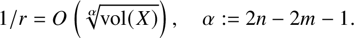 $$ \begin{align} 1/r = O\left(\sqrt[\alpha]{\operatorname{vol}(X)}\right), \quad \alpha:=2n-2m-1. \end{align} $$
The proof is based on the fact that the volume of a complex analytic set passing through the origin of a ball of radius  $\varepsilon $ is at least
  $\operatorname {const}\cdot \varepsilon ^{2\dim X}$. An analytic set that meets many disjoint balls must therefore have large volume. We remark that this is an essentially complex-geometric statement which fails in the real setting.
Having established the estimate (20), we see that to construct a reasonably large Weierstrass polydisc around the origin for  ${\mathcal B}\cap V$ (and then cover
  ${\mathcal B}^{2}$ by a simple subdivision argument), it is enough to estimate the volume of this set. Moreover, a simple integral estimate shows that having found such a Weierstrass polydisc
  $\Delta $, the multiplicity
  $e(X,\Delta )$ is also upper bounded in terms of
  $\operatorname {vol}({\mathcal B}\cap V)$. We reduce the estimation of this volume, using a complex analytic version of Crofton’s formula, to counting the intersections of
  ${\mathcal B}\cap V$ with all linear planes of complementary dimension. We realise these planes as leaves of a new (lower dimensional) foliated space and finish the proof by inductive application of Theorem 1.
1.6.3 Under the rug
The two inductive steps of our proof are carried out by restricting our foliation  ${\mathcal F}\,$ to its linear subfoliations (where the leaves are given by linear subspaces, in the
  ${\boldsymbol \xi }$-variables, of the original leaves). It may happen coincidentally that new unlikely intersections are created in this process. For example, if
  $P_{1},P_{2}$ are two polynomial equations intersecting properly with a two-dimensional leaf
  ${\mathcal L}_{p}$, it may happen that the restriction of
  $P_{1}$ to some one-dimensional
  ${\boldsymbol \xi }$-linear subspace of
  ${\mathcal L}_{p}$ vanishes identically. In this case one cannot control the
  $\log \operatorname {dist}^{-1}({\mathcal B},\Sigma _{V})$ term coming up in the induction.
To avoid this problem, we note that the particular choice of linear  ${\boldsymbol \xi }$-coordinates plays no special role in the argument, and one can use any other parametrisation (sufficiently close to the identity to maintain control over the distortion of the
  ${\boldsymbol \xi }$-unit balls). We therefore replace the vector fields
  ${\boldsymbol \xi }$ with a new tuple
  $\tilde {\boldsymbol \xi }$ generating the same foliation
  ${\mathcal F}$ but producing a different parametrisation of the leaves. We show that for a sufficiently generic choice of
  $\tilde {\boldsymbol \xi }$, one can avoid creating new unlikely intersections in any of the linear sections considered in the proof. The main technical difficulty is to show that
  $\tilde {\boldsymbol \xi }$ can be constructed with
  $\delta _{\boldsymbol \xi }=\operatorname {poly}\left (\delta _{\boldsymbol \xi },\delta _{V}\right )$.
1.6.4 Counting algebraic points
Having proved the general results on counting intersection points between algebraic varieties and leaves and covering such intersections with a bounded number of Weierstrass polydiscs, one can attempt to approach a Pila–Wilkie-type counting theorem using the strategy in [Reference Binyamini and Novikov11, Reference Binyamini and Novikov12]. A direct application of this strategy yields adequate estimates for the algebraic points in a fixed number field (as a function of height) but fails to produce such estimates when one fixes only the degree of the number field. To achieve this greater generality, we use an alternative approach suggested by Wilkie [Reference Wilkie53], which replaces the interpolation determinant method by a use of the Thue–Siegel lemma. We remark that Habegger has used this approach in his work on an approximate Pila–Wilkie-type theorem [Reference Habegger29], and our result is influenced by his idea. Similar ideas have also been used earlier in more specific settings by Wilkie [Reference Wilkie52] and Masser (see [Reference Masser34] and [Reference Zannier and Masser55, Appendix F]).
Since we, unlike Wilkie and Habegger, use Weierstrass polydiscs in place of the traditional  $C^{r}$-smooth parametrisation, some technical preparations parallel to [Reference Habegger29, Reference Wilkie53] must be made. This material is developed in Section 6.1.
2 Multiplicity operators and local geometry on ${\mathcal F}$

Let  $F=(F_{1},\dotsc ,F_{n})$ denote an n-tuple of holomorphic functions in some domain
  $\Omega \subset {\mathbb C}^{n}$. In [Reference Binyamini and Novikov10], a collection
  $\left \{M_{B}^{\alpha }\right \}$ of ‘basic multiplicity operators’ of order k is defined. These are partial differential operators of order k – that is, polynomial combinations of
  $F_{1},\dotsc ,F_{n}$ and their first k derivatives.Footnote 1 We will usually denote a multiplicity operator of order k by
  $M^{\smash {(k)}}$ and write
  $M^{\smash {(k)}}_{p}(F)$ for
  $\left [M^{\smash {(k)}}(F)\right ](p)$.
The key defining property of the multiplicity operators is the following. Denote by  $\operatorname {mult}_{p} F$ the multiplicity of p as a common zero of
  $F_{1},\dotsc ,F_{n}$ (with
  $\operatorname {mult}_{p}F=0$ if p is not a common zero and
  $\operatorname {mult}_{p} F=0$ if p is a nonisolated zero).
Proposition 7 [Reference Binyamini and Novikov10, Proposition 5]
We have  $\operatorname {mult}_{p} F>k$ if and only if
  $M^{\smash {(k)}}_{p}F=0$ for all multiplicity operators of order k.
2.1 Multiplicity operators and Weierstrass polydiscs
In this section we denote by  $B\subset {\mathbb C}^{n}$ the unit ball. The norm
  $\left \lVert \cdot \right \rVert $ always denotes the maximum norm. We will need the following basic lemma on multiplicity operators:
Lemma 8. Set  $F_{1},\dotsc ,F_{n}:B\to D(1)$. Suppose that
  $s=\left \lvert M^{\smash {(k)}}_{0}F \right \rvert \neq 0$ for some multiplicity operator
  $M^{\smash {(k)}}$. Let
  $\ell \in ({\mathbb C}^{n})^{*}$ have unit norm and set
  $0<\rho <s$. Then there is a ball
  $B^{\prime }$ around the origin of radius at least
  $s/\operatorname {poly}_{n}(k)$ and a union of at most k discs
  $U_{\rho }$ of total radius at most
  $\operatorname {poly}_{n}(k)\cdot \rho $, such that
 $$ \begin{align} {\mathbf z}\in B^{\prime}\setminus\ell^{-1}\left(U_{\rho}\right) \implies \log \left\lVert F({\mathbf z}) \right\rVert \ge (k+1)\log\rho-\operatorname{poly}_{n}(k). \end{align} $$
Proof. The statement follows from the proof of [Reference Binyamini and Novikov10, Theorem 2]. To see this, it suffices to check in the proof that the various constants appearing there indeed have logarithms of order  $\operatorname {poly}_{n}(k)$. This boils down to estimating the constants
  $C_{k}$ and
  $C^{D}_{n,k}$. The former is given explicitly in [Reference Binyamini and Yakovenko16, Lemma 4.1], in the form
  $C_{k}=2^{-O(k)}$. The latter arises in the proof of [Reference Binyamini and Novikov10, Proposition 6] from applying Cramer’s rule to a determinant of size
  $\operatorname {poly}_{n}(k)$, and is easily seen to satisfy
  $\log C^{D}_{n,k}=\operatorname {poly}_{n}(k)$.
We now state a result relating the multiplicity operators to the construction of a Weierstrass polydisc for a curve:
Lemma 9. Set  $F_{1},\dotsc ,F_{n-1}:B\to D(1)$. Suppose that
  $s=\left \lvert M^{\smash {(k)}}_{0}F \right \rvert \neq 0$ for some
  $(n-1)$-dimensional multiplicity operator
  $M^{\smash {(k)}}$ with respect to the variables
  ${\mathbf w}=z_{2},\dotsc ,z_{n}$. Then there exists a Weierstrass polydisc for the set
  $\{F=0\}$ in the standard coordinates
  $\Delta =D(r_{1})\times \dotsb \times D(r_{n})$ with all the radii satisfying
 $$ \begin{align} \log r_{i} \ge \operatorname{poly}_{n}(k) \log s. \end{align} $$
Proof. We claim that one can find a polydisc  $\Delta _{w}=D(r_{2})\times \dotsb \times D(r_{n})$ such that
 $$ \begin{align} \log \left\lVert F(0,{\mathbf w}) \right\rVert\ge (k+1)\log s-\operatorname{poly}_{n}(k) \text{ for every }{\mathbf w}\in\partial\Delta_{w}, \end{align} $$
and moreover,
 $$ \begin{align} \log r_{i} \ge \operatorname{poly}_{n}(k)\log s \text{ for } i=2,\dotsc,n. \end{align} $$
To prove this, apply Lemma 8 to  $F(0,{\mathbf w})$, with
  $\ell $ given by each of the
  ${\mathbf z}_{2},\dotsc ,{\mathbf z}_{n}$-coordinates with a suitable choice
  $\rho =s/\operatorname {poly}_{n}(k)$, and then choose
  $\Delta _{w}$ to be a polydisc inside the balls
  $B^{\prime }$ and with each
  $\partial D\left (r_{j}\right )$ disjoint from the set
  $U_{\rho }$ obtained for
  $\ell ={\mathbf z}_{j}$.
Since  $F_{1},\dotsc ,F_{n-1}$ have unit maximum norms, their derivatives are bounded by
  $O(1)$ in
  $B^{2}$ by the Cauchy estimate. It follows that
  $F(z,{\mathbf w})$ cannot vanish on
  $\partial \Delta _{w}$ for
  $z\in D(r_{1})$, where
 $$ \begin{align} \log r_{1}\sim (k+1)\log s-\operatorname{poly}_{n}(k), \end{align} $$
so  $D(r_{1})\times \Delta _{w}$ indeed gives a Weierstrass polydisc satisfying the final condition
  $\log r_{1}\ge \operatorname {poly}_{n}(k) \log s$.
Suppose that  $\Gamma \subset {\mathbb C}^{n}$ is an analytic curve,
  $\Delta =D_{z}\times \Delta _{w}$ is a Weierstrass polydisc for
  $\Gamma $ and
  $G:\Delta \to {\mathbb C}$ is holomorphic.
Definition 10. We define the analytic resultant of G with respect to  $\Delta $ to be the holomorphic function
  ${\mathcal R}_{\Delta ,\Gamma }(G):D_{z}\to {\mathbb C}$ given by
 $$ \begin{align} \left[{\mathcal R}_{\Delta,\Gamma}(G)\right](z) = \prod_{w:(z,w)\in\Gamma\cap\Delta} G(z,w). \end{align} $$
Our second result concerns a lower estimate for analytic resultants in terms of multiplicity operators.
Lemma 11. Let  $F_{1},\dotsc ,F_{n}:B\to D(1)$ be holomorphic. Set
  $\Gamma =\{F_{1}=\dotsb =F_{n-1}=0\}$ and suppose that
  $\Delta =D(r)\times \Delta _{w}\subset B$ is a Weierstrass polydisc in the standard coordinates for
  $\Gamma $ with multiplicity
  $\mu $. Suppose that
  $s=\left \lvert M^{\smash {(k)}}_{0}(F)\right \rvert \neq 0$ for some multiplicity operator
  $M^{\smash {(k)}}$. Set
  $0<\rho <s$. Then for z in a ball of radius
  $\Omega _{n}(s)$ around the origin and outside a union of balls of radius
  $O_{n}(\rho )$, we have
 $$ \begin{align} \log \lvert R(z)\rvert> \mu\cdot((k+1)\log\rho-\operatorname{poly}_{n}(k)), \quad R:={\mathcal R}_{\Delta,\Gamma}(F_{n}):D(r)\to{\mathbb C}. \end{align} $$
Proof. Apply Lemma 8 with  $\ell ={\mathbf z}_{1}$ and
  $\rho $. We see that
  $\log \left \lVert F({\mathbf z}) \right \rVert \ge (k+1)\log \rho -\operatorname {poly}_{n}(k)$ in a ball
  $B^{\prime }$ of radius
  $\Omega _{n}(s)$ whenever
  ${\mathbf z}_{1}$ lies outside
  $U_{\rho }$. In particular, this is true for the
  $\mu $ points
  $({\mathbf z}_{1},w)$ where
  $F_{1},\dotsc ,F_{n-1}$ vanish. At these points we have
  $\log \lvert F_{n}({\mathbf z})\rvert =\log \left \lVert F({\mathbf z}) \right \rVert $. Taking the product over the
  $\mu $ different points, as in the definition of R, proves the statement.
2.2 Multiplicity operators along ${\mathcal F}$

When  $P=(P_{1},\dotsc ,P_{n})\in {\mathcal O}({\mathbb M})^{n}$, we may apply the multiplicity operator
  $M^{\smash {(k)}}$ to P by evaluating the derivatives along
  ${\boldsymbol \xi }_{1},\dotsc ,{\boldsymbol \xi }_{n}$. This amounts to computing, for each point
  $p\in {\mathbb M}$, the multiplicity operator of
  $P{\vert _{{\mathcal L}}}_{p}$ in the
  ${\boldsymbol \xi }$-chart.
Lemma 12. For any multiplicity operator  $M^{\smash {(k)}}$, we have
 $$ \begin{align} \delta\left(M^{\smash{(k)}} P\right) = \operatorname{poly}\left(\delta_{P},\delta_{\boldsymbol\xi},k\right). \end{align} $$
Proof. This is a simple computation, owing to the fact that  $M^{\smash {(k)}}$ is defined by expanding a determinant of size
  $\operatorname {poly}_{n}(k)$ with entries defined in terms of P and its
  ${\boldsymbol \xi }$-derivatives up to order k.
We will require the following result of Gabrielov and Khovanskii [Reference Gabrielov and Khovanskii26]:
Theorem 5. With P as before and  $p\in {\mathbb M}\setminus \Sigma _{V(P)}$,
 $$ \begin{align} \operatorname{mult}_{p} P < \operatorname{poly}(\deg{\boldsymbol\xi}, \deg P). \end{align} $$
As a consequence, we have the following:
Proposition 13. Let  $V\subset {\mathbb M}$ be a complete intersection
  $V=V(P_{1},\dotsc ,P_{m})$ with
  $m\le n$. Then
 $$ \begin{align} \delta(\Sigma_{V}) = \operatorname{poly}\left(\delta_{\boldsymbol\xi},\delta_{V}\right). \end{align} $$
Moreover, if  $m=n$, then
  $\Sigma _{V}$ is set-theoretically cut out by the functions
  $\left \{M^{\smash {(k)}}(P)\right \}$, where
  $M^{\smash {(k)}}$ varies over all multiplicity operators of order
  $k=\operatorname {poly}(\deg {\boldsymbol \xi },\deg P)$.
Proof. We have  $p\in \Sigma _{V}$ if and only if
  $p\in \Sigma _{\mathcal F}$ or
  $\dim \left ({\mathcal L}_{p}\cap V\right )>n-m$. Since clearly
  $\delta (\Sigma _{\mathcal F})=\operatorname {poly}\left (\delta _{\boldsymbol \xi }\right )$, we only have to write equations for the latter condition. This is equivalent to the statement that for every
  ${\boldsymbol \xi }$-linear subspace of
  ${\mathcal L}_{p}$ of dimension m, the intersection
  $V\cap L$ is nonisolated – that is, has infinite multiplicity. We express this using multiplicity operators as follows.
Let  ${\mathbf c}^{1},\dotsc ,{\mathbf c}^{m}$ be n-tuples of indeterminate coefficients and let
 $$ \begin{align} {\boldsymbol\xi}_{\mathbf c}=\left({\mathbf c}^{1}\cdot{\boldsymbol\xi},\dotsc,{\mathbf c}^{m}\cdot{\boldsymbol\xi}\right) \end{align} $$
denote the subfoliation of  ${\boldsymbol \xi }$ generated by the corresponding linear combinations. Then for every
  $p\in {\mathbb M}\setminus \Sigma _{\mathcal F}$, we obtain a linear subspace
  ${\mathcal L}_{p,{\mathbf c}}\subset {\mathcal L}_{p}$ and we seek to express the condition that
  ${\mathcal L}_{p,{\mathbf c}}\cap V$ is an intersection of infinite multiplicity for every
  ${\mathbf c}$. By Theorem 5, if the multiplicity of the intersection is finite, then it is bounded by
  $k=\operatorname {poly}(\deg {\boldsymbol \xi },\deg P)$. It is enough to express the condition that the multiplicity exceeds this number for every
  ${\mathbf c}$. According to Proposition 7, for every fixed value of
  ${\mathbf c}$ this condition can be expressed by considering all multiplicity operators
  $M^{\smash {(k)}}(P)$ with respect to
  ${\boldsymbol \xi }_{\mathbf c}$. Expanding these expressions with respect to the variables
  ${\mathbf c}$ and taking the ideal generated by all the coefficients, we obtain equations for the vanishing for every
  ${\mathbf c}$. The estimates on the degrees and heights of these equations follow easily from Lemma 12.
We record a useful corollary of Proposition 13:
Corollary 14. Let  $V=V(P_{1},\dotsc ,P_{n})$ be a complete intersection and set
  $p\in {\mathbb B}$. There exists a multiplicity operator
  $M^{\smash {(k)}}$ of order
  $k=\operatorname {poly}(\deg {\boldsymbol \xi },\deg V)$ such that
 $$ \begin{align} \log\left\lvert M^{\smash{(k)}}_{p}(P)\right\rvert \ge \operatorname{poly}\left(\delta_{\boldsymbol\xi},\delta_{V}\right)\cdot \log\operatorname{dist}(p,\Sigma_{V}). \end{align} $$
Proof. According to Proposition 13, the set  $\Sigma _{V}$ is set-theoretically cut out by the multiplicity operators
  $M^{\smash {(k)}}(P)$ as before. Since the degrees and heights of these polynomials are bounded according to Lemma 12, the result follows by application of the Diophantine Łojasiewicz inequality due to Brownawell [Reference Brownawell20].
3 Covering by Weierstrass polydiscs
Let  $B\subset {\mathbb C}^{n}$ denote the unit ball around the origin and
  $X\subset B$ an analytic subset of pure dimension m. In this section we prove that one can find a Weierstrass polydisc around the origin for X, where the size of the polydisc depends on the volume of X.
For a subset  $A\subset {\mathbb C}^{n}$, denote by
  $N(A,\varepsilon )$ the size the smallest
  $\varepsilon $-net in A and by
  $S(A,\varepsilon )$ the size of the maximal
  $\varepsilon $-separated set in A. One easily checks that
 $$ \begin{align} S(A,2\varepsilon) \le N(A,\varepsilon) \le S(A,\varepsilon). \end{align} $$
Lemma 15. For  $\varepsilon \le 1$, we have
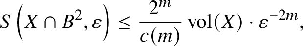 $$ \begin{align} S\left(X\cap B^{2},\varepsilon\right) \le \frac{2^{m}}{c(m)} \operatorname{vol}(X)\cdot \varepsilon^{-2m}, \end{align} $$
where  $c(m)$ denotes the volume of the unit ball in
  ${\mathbb C}^{m}$.
Proof. Suppose  $S\subset X\cap B^{2}$ is an
  $\varepsilon $-separated set. Then balls
  $B_{p}:=B(p,\varepsilon /2)$ for
  $p\in S$ are disjoint, and according to [Reference Chirka and Hoksbergen19, Theorem 15.3] we have
 $$ \begin{align} \operatorname{vol}\left(X\cap B_{p}\right) \ge c(n)(\varepsilon/2)^{2m}. \end{align} $$
The conclusion follows because the disjoint union of these sets is contained in X.
Let the unit circle  $S^{1}\subset {\mathbb C}$ act on
  ${\mathbb C}^{n}$ by scalar multiplication.
Lemma 16. Let  $A\subset B$. Then
 $$ \begin{align} N\left(S^{1}\cdot A,2\varepsilon\right) \le (1+\lfloor \pi/\varepsilon \rfloor) \cdot N(A,\varepsilon). \end{align} $$
Proof. Build a  $2\varepsilon $-net for
  $S^{1}\cdot A$ by multiplying an
  $\varepsilon $-net in
  $S^{1}$ by an
  $\varepsilon $-net in A.
The following proposition is our key technical result:
Proposition 17. There exists a ball  $B^{\prime }\subset B$ of radius
  $\varepsilon $ disjoint from
  $S^{1}\cdot X$, where
 $$ \begin{align} 1/\varepsilon = O_{n}\left(\sqrt[\alpha]{\operatorname{vol}(X)}\right), \quad \alpha:=2n-2m-1. \end{align} $$
Proof. Set  $X^{\prime }=S^{1}\cdot \left (X\cap B^{2}\right )$. By Lemmas 15 and 16, we have
 $$ \begin{align} N(X^{\prime},\varepsilon) = O_{n}\left(\operatorname{vol}(X)\varepsilon^{-2m-1}\right). \end{align} $$
On the other hand, clearly
 $$ \begin{align} S\left(B^{2},\varepsilon\right) = \Theta_{n}\left(\varepsilon^{-2n}\right). \end{align} $$
Suppose that N is an  $\varepsilon $-net for
  $X^{\prime }$ and S is a
  $4\varepsilon $-separated set in
  $B^{2}$. Suppose that every
  $\varepsilon $-ball
  $B_{p}$ around a point
  $p\in S$ meets
  $X^{\prime }$. Then the
  $B_{p}^{1/2}$ meets N. Since S is
  $4\varepsilon $-separated, no two balls
  $B_{p}^{1/2},B_{q}^{1/2}$ for
  $p,q\in S$ meet the same point of N, so
  $\#S\le \#N$. In conclusion, as soon as we have
  $S\left (B^{2},\varepsilon \right )>N(X^{\prime },\varepsilon )$, there exists an
  $\varepsilon $-ball
  $B_{p}$ that does not meet
  $X^{\prime }$.
As a corollary, we obtain our main result for this section:
Corollary 18. There exists a Weierstrass polydisc  $\Delta \subset B$ for X which contains
  $B^{\eta }$, where
  $\eta =\operatorname {poly}_{n}(\operatorname {vol}(X))$. Moreover,
  $e(X,\Delta )=\operatorname {poly}_{n}(\operatorname {vol}(X))$.
Proof. The proof of the first part is the same as [Reference Binyamini and Novikov12, Theorem 7], where we replace the use of Vitushkin’s formula and sub-Pfaffian arguments with Proposition 17. Briefly, after finding a ball  $B^{\prime }$ disjoint from
  $S^{1}\cdot X$, one notes that
  $B^{\prime }$ contains a set which has the form
  $\Delta \times \partial D(r)$ in some unitary coordinate system, where the radii of
  $\Delta $ and
  $D(r)$ are roughly the same as the radius of
  $B^{\prime }$. It is then easy to reduce the problem to finding a Weierstrass polydisc for
  $\pi (X)$ inside
  $\Delta $. Since
  $\pi (X)$ is again an analytic set and
  $\operatorname {vol}(\pi (X))\le \operatorname {vol}(X)$, the proof is concluded by induction over the dimension.
For the second part, write
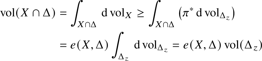 $$ \begin{align} \operatorname{vol}(X\cap\Delta) &= \int_{X\cap\Delta} \,\mathrm d\operatorname{vol}_{X} \ge \int_{X\cap\Delta} \left(\pi^{*}\,\mathrm d\operatorname{vol}_{\Delta_{z}}\right) \notag \\ &= e(X,\Delta) \int_{\Delta_{z}} \,\mathrm d\operatorname{vol}_{\Delta_{z}} = e(X,\Delta) \operatorname{vol}(\Delta_{z}) \end{align} $$
and note that  $\operatorname {vol}(\Delta _{z})^{-1}=\operatorname {poly}_{n}(\operatorname {vol}(X))$, by what was already proved.
4 Achieving general position
Let  $V\subset {\mathbb M}$ be a variety of pure dimension m. We will assume until Section 4.5 that V is a complete intersection variety defined by
  $Q_{1},\dotsc ,Q_{n-m}\in {\mathcal O}({\mathbb M})$. In Section 4.5 we prove a result that allows us to reduce the general case to the case of complete intersections.
As explained in Section 1.6, a part of our inductive scheme involves studying intersections between the variety defined by  $Q_{1},\dotsc ,Q_{k}$ and subfoliations of
  ${\mathcal F}$ defined by k-dimensional linear subspaces of
  $\langle \xi _{1},\dotsc ,\xi _{n}\rangle $. To carry this out uniformly, we add the coefficients of such a linear combination to
  ${\mathbb M}$. It may happen that the process of restricting to a linear subfoliation introduces new unlikely intersections (e.g., if
  $Q_{1}$, while not vanishing identically on a leaf, happens to vanish on a linear hyperplane in the
  ${\boldsymbol \xi }$-coordinates). To avoid such degeneracies, we perturb the time parametrisation, changing the fields
  ${\boldsymbol \xi }$ while preserving the leaves
  ${\mathcal L}_{p}$ themselves. We show that this can be done while preserving suitable control over
  $\delta _{\boldsymbol \xi }$.
4.1 Parametrising linear subfoliations
Set  $k\le n$ and let
  $A(n,k)$ denote the affine variety of full rank matrices
  $({\boldsymbol \alpha }_{1},\dotsc ,{\boldsymbol \alpha }_{k})\in \operatorname {Mat}_{n\times k}$. Define
  $L_{k}{\mathbb M}:=A(n,k)\times {\mathbb M}$ and consider the vector fields
 $$ \begin{align} L_{k}({\boldsymbol\xi})_{i} = {\boldsymbol\alpha}_{i}\cdot{\boldsymbol\xi}, \quad i=1,\dotsc,k. \end{align} $$
The leaves of  $L_{k}{\mathbb M}$ with
  $L_{k}({\boldsymbol \xi })$ correspond to the leaves obtained by choosing a k-dimensional subspace of
  $\langle {\boldsymbol \xi }_{1},\dotsc ,{\boldsymbol \xi }_{n}\rangle $ and using it to span a k-dimensional subfoliation of
  ${\mathcal F}$.
4.2 Main statement
Our goal is to construct an affine variety  $\tilde {\mathbb M}:=N\times {\mathbb M}$ depending only on
  ${\mathbb M}$, and vector fields
  $\tilde {\boldsymbol \xi }$ depending on
  ${\mathbb M},V$, with the following properties:
1. If we denote by
$\pi _{\mathbb M}:\tilde {\mathbb M}\to {\mathbb M}$ the projection and by $\phi _{p},\tilde \phi _{a,p}$ the ${\boldsymbol \xi },\tilde {\boldsymbol \xi }$ charts, respectively, then for any $(a,p)\in \tilde {\mathbb M}$ we have $\pi _{\mathbb M}\circ \tilde \phi _{a,p}=\phi _{p}\circ \Phi _{a,p}$, where $\Phi _{a,p}$ is the germ of a self map of $({\mathbb C}^{n},0)$. In particular, ${\mathcal L}_{p}=\pi _{\mathbb M}\left ({\mathcal L}_{a,p}\right )$.2. Whenever
$\phi _{p}$ extends to the unit ball, the germ $\Phi _{a,p}$ extends to $B^{2} $ and (42)In other words, the reparametrisation is close to the identity.$$ \begin{align} \left\lVert \Phi_{a,p}-\operatorname{id} \right\rVert_{B^{2}}<0.1. \end{align} $$3. We have effective estimates
(43)$$ \begin{align} \deg\tilde{\boldsymbol\xi}=\deg{\boldsymbol\xi}+O(1), \qquad h\left(\tilde{\boldsymbol\xi}\right)=\operatorname{poly}\left(\delta_{\boldsymbol\xi},\deg V\right). \end{align} $$4. For
$k=\operatorname {codim} V$, if we set $\tilde {\mathbb M}_{k}:=L_{k}\tilde {\mathbb M}$ and denote by $\tilde V$ the natural pullback to $\tilde {\mathbb M}_{k}$, then (44)In other words, no ‘new’ unlikely intersections are formed when considering linear subfoliations of$$ \begin{align} \pi_{\mathbb M}\left(\Sigma_{\tilde V}\right)\subset \Sigma_{V}. \end{align} $$$\tilde {\mathbb M},\tilde {\boldsymbol \xi }$.


We also remark that one can similarly achieve general position with respect to any  $O(1)$ different varieties
  $V_{i}\subset {\mathbb M}$, by the same argument.
4.3 Polynomial time reparametrisation
Fix  $D\in {\mathbb N}$ and let
  ${\mathcal M}_{D}$ denote the space of polynomial maps
  $\Phi :{\mathbb C}^{n}\to {\mathbb C}^{n}$ with coordinate-wise degree at most D. Let
  $P_{D}({\mathbb M})$ denote the affine variety obtained from
  ${\mathcal M}_{D}\times {\mathbb C}^{n}_{s}\times {\mathbb M}$ by imposing the condition
  $\det \tfrac {\partial \Phi ({\mathbf s})}{\partial {\mathbf s}}\neq 0$, where we use
  $\Phi $ for the coordinate on
  ${\mathcal M}_{D}$ and
  ${\mathbf s}$ for the coordinate on
  ${\mathbb C}^{n}$. Consider the vector fields
 $$ \begin{align} P_{D}(\xi_{i}) = \tfrac{\partial}{\partial{\mathbf s}_{i}} + \tfrac{\partial\Phi({\mathbf s})}{\partial{\mathbf s}}\cdot{\boldsymbol\xi}. \end{align} $$
Then the local  $P_{D}({\boldsymbol \xi })$-chart at a point
  $(\Phi ,a,p)$ is given by
 $$ \begin{align} \phi_{\Phi,a,p}({\mathbf x}) = \left(\Phi,a+{\mathbf x},\phi_{p}(\Phi(a+{\mathbf x})-\Phi(a))\right). \end{align} $$
In particular, the projection of the leaf  $P_{D}({\mathcal L})_{\Phi ,a,p}$ to
  ${\mathbb M}$ is the germ
  ${\mathcal L}_{p}$, but the time parametrisation is adjusted according to
  $\Phi $ around a.
4.4 Codimension of unlikely intersection
Set
 $$ \begin{align} \tilde {\mathbb M} = L_{k}(P_{D}{\mathbb M})= A(n,k)\times{\mathcal M}_{D}\times{\mathbb C}^{n}_{s}\times{\mathbb M}. \end{align} $$
Denote by  $\tilde V$ the pullback of V to
  $\tilde {\mathbb M}$.
Lemma 19. Let  $p\in {\mathbb M}\setminus \Sigma _{V}$,
  $A\in A(n,k)$ and
  $a\in {\mathbb C}^{n}_{s}$. Then the set
 $$ \begin{align} \left\{\Phi\in{\mathcal M}_{D} : (A,\Phi,a,p)\in\Sigma_{\tilde V} \right\}\subset{\mathcal M}_{D} \end{align} $$
is algebraic of codimension at least D.
Proof. Algebraicity follows from Proposition 13. Replacing a by  $0$ and
  $\Phi ({\mathbf x})$ by
  $\Phi (a+{\mathbf x})-\Phi (a)$, we may assume without loss of generality that
  $a=0$. Similarly, replacing A by
  $({\boldsymbol \xi }_{1},\dotsc ,{\boldsymbol \xi }_{k})$ and
  $\Phi ({\mathbf x})$ by its appropriate linear change of variable, we may assume without loss of generality that
  $A=({\boldsymbol \xi }_{1},\dotsc ,{\boldsymbol \xi }_{k})$.
Denote  $\Phi ^{\prime }_{j}=\Phi _{j}-\Phi _{j}(0)$. Then the leaf at
  $(A,\Phi ,0,p)$ is defined by
 $$ \begin{align} (A,\Phi,0)\times{\mathcal L}_{p}^{\prime}, \quad {\mathcal L}_{p}^{\prime}={\mathcal L}_{p}\cap\left\{\Phi^{\prime}_{k+1}=\dotsb=\Phi^{\prime}_{n}=0\right\}. \end{align} $$
We must check when the intersection of  ${\mathcal L}_{p}^{\prime }$ and V is a complete intersection. It is enough to bound the codimension of the condition that
  $\Phi ^{\prime }_{k+1}$ vanishes identically on (a component of)
  ${\mathcal L}_{p}\cap V$, that
  $\Phi ^{\prime }_{k+2}$ vanishes identically on (a component of)
  ${\mathcal L}_{p}\cap \left \{\Phi ^{\prime }_{k+1}=0\right \}\cap V$ and so on.
From the foregoing we conclude that it is enough to prove the following simple claim: let  $\gamma \subset ({\mathbb C}^{n},0)$ be the germ of an analytic curve. Then the set of polynomials of degree at most D without a free term vanishing identically on
  $\gamma $ has codimension at least D. Note that this set is linear. Choose t to be a (linear) coordinate on
  ${\mathbb C}^{n}$ which is nonconstant on
  $\gamma $. Then clearly
  $t,\dotsc ,t^{D}$ are linearly independent on
  $\gamma $, and the claim follows.
Now choose  $D=\dim A(n,k)+n+\dim {\mathbb M}+1$. Denote by
  $\pi _{\Phi }:\tilde {\mathbb M}\to {\mathcal M}_{D}$ the projection. Then by a dimension-counting argument using Lemma 19, the codimension of
  $\pi _{\Phi }\left (\Sigma _{\tilde V}\right )$ is positive. By Proposition 13 the degree of the Zariski closure
  $Z:=\operatorname {Clo}\pi _{\Phi }\left (\Sigma _{\tilde V}\right )$ is bounded by
  $\operatorname {poly}(\deg V,\deg {\boldsymbol \xi })$. If we choose any
  $\Phi _{0}\not \in Z$ and restrict
  $\tilde {\mathbb M}$ to
  $\Phi =\Phi _{0}$, then the final condition in Section 4.2 is satisfied by definition. It remains only to show that
  $\Phi _{0}$ can be chosen close to the identity map and with appropriately bounded height. This follows immediately from the following general statement:
Lemma 20. Let  $Z\subset {\mathbb A}^{N}$ be an affine subvariety of total degree at most d. Then there exists a point
  ${\mathbf x}\in {\mathbb Q}^{N}\setminus Z$ satisfying
  $\left \lVert {\mathbf x} \right \rVert _{\infty }\le 1$ and
  $H({\mathbf x})\le d$.
Proof. Let  $C\subset {\mathbb C}$ denote the set of points z such that Z has a component contained in
  $\{{\mathbf x}_{1}=z\}$. Clearly
  $\#C\le d$. Choose
  $x\in [-1,1]\cap ({\mathbb Q}\setminus C)$ with
  $H(x)\le d$. The claim now follows by induction over N for the variety
  $Z\cap \{{\mathbf x}_{1}=x\}$, naturally identified as a subvariety of
  ${\mathbb A}^{N-1}$.
4.5 Generic choice of a complete intersection
Let  $V\subset {\mathbb M}$ be a variety defined over
  ${\mathbb K}$. In this section we show that one can choose a complete intersection W containing V with
  $\Sigma _{W}$ being ‘as small as possible’ and with effective control over
  $\delta _{W}$. We will need the following elementary lemma:
Lemma 21. The variety V is set-theoretically cut out by a collection of polynomial equations  $P_{1},\dotsc ,P_{S}$ with
  $\delta (P_{\alpha })=\operatorname {poly}(\delta _{V})$ and S depending only on the dimension of the ambient space of
  ${\mathbb M}$.
Proof. Recall that we define  $h(V)$ in terms of the height of its Chow coordinates. The statement thus follows from a classical construction due to Chow and van der Waerden that produces a canonical system of equations for V in terms of the Chow coordinates [Reference Gel’fand, Kapranov and Zelevinsky27, Corollary 3.2.6].
The following is our main result for this section:
Proposition 22. Let  $0\le m\le \dim {\mathbb M}$ be an integer. There exists a complete intersection W of pure codimension m that contains V and satisfies
  $\delta _{W}=\operatorname {poly}\left (\delta _{\boldsymbol \xi },\delta _{V}\right )$ and
 $$ \begin{align} \Sigma_{W} = \left\{p\in{\mathbb M} : \dim\left(V\cap{\mathcal L}_{p}\right)>n-m\right\}. \end{align} $$
Proof. We remark that the inclusion  $\subset $ in equation (50) is trivial. Suppose that we have already constructed a complete intersection
  $W_{k}$ of pure codimension
  $k<m$ satisfying the conditions. We will show how to choose a polynomial equation P vanishing on V, with
  $\delta _{P}$ bounded, such that
  $W_{k+1}=W\cap V(P)$ satisfies
 $$ \begin{align} \Sigma_{W_{k+1}} = \left\{p\in{\mathbb M} : \dim\left(V\cap{\mathcal L}_{p}\right)>n-k-1\right\}. \end{align} $$
The claim then follows by induction on k.
Let  $D=\dim {\mathbb M}+1$ and let
  ${\mathcal P}_{D}$ denote the space of polynomials in the ambient space of
  ${\mathbb M}$ of degree at most D. Consider
  $\tilde {\mathbb M}:={\mathcal P}_{D}^{S}\times {\mathbb M}$ and let
  $\tilde P\in {\mathcal O}\left (\tilde {\mathbb M}\right )$ be given by
 $$ \begin{align} \tilde P(Q_{1},\dotsc,Q_{S},\cdot) = Q_{1}P_{1}+\dotsb+Q_{S}P_{S}, \quad (Q_{1},\dotsc,Q_{S})\in{\mathcal P}_{D}^{S}. \end{align} $$
Set  $\tilde W_{k+1}=\tilde W_{k}\cap V\left (\tilde P\right )$, where
  $\tilde W_{k}:={\mathcal P}_{D}^{S}\times W_{k}.$
Let p satisfy  $\dim \left (V\cap {\mathcal L}_{p}\right )<n-k$. By assumption,
  $p\not \in \Sigma _{W_{k}}$. We claim that the codimension in
  ${\mathcal P}_{D}^{S}$ of the set
 $$ \begin{align} \left\{ Q\in{\mathcal P}_{D}^{S} : (Q,p)\in\Sigma_{\tilde W_{k+1}}\right\} \end{align} $$
is at least D. Indeed, the condition is equivalent to the fact that  $\tilde P$ does not vanish identically on any of the irreducible components of
  ${\mathcal L}_{p}\cap W_{k}$. It is enough to check the codimension for each component C separately. Since V is set-theoretically cut out by
  $P_{1},\dotsc ,P_{S}$ and
  $\dim \left (V\cap {\mathcal L}_{p}\right )<n-k$, one of the polynomials
  $P_{j}$ – say, without loss of generality,
  $P_{1}$ – does not vanish identically on C. Then for any fixed value of
  $Q_{2},\dotsc ,Q_{S}$, at most one value of
  $Q_{1}{\vert _{C}}$ can give
  $\tilde P{\vert _{C}}\equiv 0$, and we have already seen in the proof of Lemma 19 that the codimension of this affine linear condition is at least D.
We now finish as in Section 4.4. Namely, by Proposition 13 we see that  $\Sigma _{\tilde W_{k+1}}$ is algebraic and
 $$ \begin{align} \deg \Sigma_{\tilde W_{k+1}}=\operatorname{poly}(\deg({\boldsymbol\xi}),\deg(V)). \end{align} $$
Set  $Z=\operatorname {Clo} \pi \left (\Sigma _{\tilde W_{k+1}}\right )$, where
  $\pi :\tilde M\to {\mathcal P}_{D}^{S}$, and note that by a dimension-counting argument Z has positive codimension. Choosing a point
  $Q\not \in Z$ using Lemma 20 and setting
  $P=\tilde P(Q,\cdot )$ finishes the proof.
5 Proofs of the main theorems
In this section we prove Theorems 1 and 2 by a simultaneous induction. We will assume in both proofs that V is given by a complete intersection  $V=V(P_{1},\dotsc ,P_{m})$. For the general case, we replace V by a complete intersection W containing it, as in Proposition 22. Since
  $\Sigma _{V}=\Sigma _{W}$, the statements for V follow immediately from the statements for W.
To avoid repeating the expression  $\operatorname {poly}\left (\delta _{\boldsymbol \xi },\delta _{V},\log \operatorname {dist}^{-1}({\mathcal B},\Sigma _{V})\right )$, we will say simply that a quantity is appropriately bounded if it admits such a bound. Recall that, as explained in Section 1.2, we can and do assume that
  $R=1$.
5.1 Proof of Theorem 1
We prove Theorem 1 in dimension n assuming that it holds for dimension at most  $n-1$ and that Theorem 2 holds for dimension at most n.
Set  $V^{\prime }:=V(P_{1},\dotsc ,P_{n-1})$. Note that
  $\Sigma _{V^{\prime }}\subset \Sigma _{V}$. We start by passing to general position with respect to V and
  $V^{\prime }$ as in Section 4.2. This has the effect of slightly reparametrising the time variables, and in the new parametrisation the original balls
  ${\mathcal B},{\mathcal B}^{2}$ are contained in balls of radius slightly larger than
  $1,1/2$. However, dividing these balls into
  $O(1)$ balls and rescaling time (i.e., rescaling
  ${\boldsymbol \xi }$), we see that it is enough to prove Theorem 1 for
  ${\mathcal B},{\mathcal B}^{2}$ in the new parametrisation.
Applying Theorem 2, we construct a collection of Weierstrass polydiscs  $\{\Delta _{\alpha }\subset {\mathcal B}\}$ for
  $V^{\prime }$ such that the union of the
  $\Delta ^{2}_{\alpha }$ covers
  ${\mathcal B}^{2}$. Since
  $\#\{\Delta _{\alpha }\}$ is appropriately bounded, it will suffice to count the zeros of
  $P_{n}$ on
  $V^{\prime }$ inside each
  $\Delta ^{2}_{\alpha }$ separately. Fix one such polydisc
  $\Delta :=\Delta _{\alpha }$ and set
  $\Delta =D_{z}\times \Delta _{w}$ (in some unitary system of coordinates). We also have that
  $\mu :=e(V^{\prime }\cap {\mathcal B},\Delta )$ is appropriately bounded.
Recall the analytic resultant defined in equation (26). The zeros of  $P_{n}$ on
  $V^{\prime }$ inside
  $\Delta $ correspond (with multiplicities) to the zeros of
  ${\mathcal R}_{\Delta ,{\mathcal B}\cap V^{\prime }}(P_{n})$ in
  $D_{z}$. We want to count those zeros contained in
  $D_{z}^{2}$. Recall the following consequence of Jensen’s formula [Reference Il’yashenko and Yakovenko30]:
Proposition 23. Let  $f:\bar D\to {\mathbb C}$ be holomorphic. Denote by M (resp., m) the maximum of
  $\lvert f(z)\rvert $ on
  $\bar D$ (resp.,
  $\bar D^{2}$). Then there exists a constant C such that
 $$ \begin{align} \#\left\{z\in D^{2} : f(z)=0 \right\} \le C\cdot\log\frac M m. \end{align} $$
 We apply this proposition to  ${\mathcal R}_{\Delta ,{\mathcal B}\cap V^{\prime }}(P_{n})$ in
  $D_{z}$. We first note that M is a product of
  $\lvert P_{n}\rvert $ evaluated at
  $\mu $ points
  $p_{1},\dotsc ,p_{\mu }\in {\mathbb B}$. It is clear that
  $\log \left \lvert P_{n}\left (p_{j}\right )\right \rvert \le \operatorname {poly}(\delta (P_{n}))$, so
  $\log M$ is appropriately bounded.
It remains to show that  $\log (1/m)$ is appropriately bounded. Let
  $p_{1},\dotsc ,p_{\mu }$ denote the points of
  $V^{\prime }$ lying over the origin in
  $\Delta ^{\prime }$. Consider the multiplicity operators
  $M^{\smash {(k)}}(P_{1},\dotsc ,P_{n-1})$ with respect to the direction of the
  ${\mathbf w}$-coordinates (which we think of as a leaf of the foliated space
  $L_{n-1}{\mathbb M}$). By Corollary 14, at every point
  $p_{j}$ there is such a multiplicity operator with
  $\log \left \lvert 1/M^{\smash {(k)}}_{p_{j}}(P_{1},\dotsc ,P_{n-1})\right \rvert $ appropriately bounded in absolute value (here we use the fact that we perturbed to general position). According to Lemma 9, each point
  $p_{j}$ is the centre of a Weierstrass polydisc
  $\Delta _{j}$ in the same coordinate system, and with the logarithms of all radii appropriately bounded in absolute value.
Denote  ${\mathcal R}_{j}:={\mathcal R}_{\Delta _{j},{\mathcal B}\cap V^{\prime }}(P_{n})$. The domains of all these functions (and of
  ${\mathcal R}$ itself) contain a disc D of radius r, with
  $\log (1/r)$ appropriately bounded. Note that
 $$ \begin{align} \lvert{\mathcal R}(z)\rvert \ge \frac{\prod_{j=1,\dotsc,\mu} \left\lvert{\mathcal R}_{j}(z)\right\rvert}{e^{\operatorname{poly}\left(\delta_{\boldsymbol\xi},\delta_{V}\right)}}, \end{align} $$
since the numerator contains the value of  $P_{n}$ evaluated at every point of
  ${\mathcal B}\cap V^{\prime }$ over z (possibly more than once), and these evaluations are always bounded from above by
  $e^{\operatorname {poly}\left (\delta \left (P_{n}\right )\right )}$, as we have already seen. It will therefore suffice to find a point in D where
  $\log \left (1/\left \lvert {\mathcal R}_{j}\right \rvert \right )$ is appropriately bounded for every j. For this we use Lemma 11. Namely, the lemma shows that
  $\log \left (1/\left \lvert {\mathcal R}_{j}\right \rvert \right )$ is appropriately bounded outside a union of balls of total radius smaller than
  $r/\mu $, and taking the union over
  $j=1,\dotsc ,\mu $, one can find a point where this happens simultaneously for every j. This shows that
  $\log (1/m)$ is appropriately bounded and concludes the proof of Theorem 1.
5.2 Proof of Corollary 2
This follows immediately by applying Proposition 22 with  $m=n$ and applying Theorem 1 to the W that one obtains.
5.3 Proof of Theorem 2
We will prove Theorem 2 in dimension n assuming that Theorem 1 holds in smaller dimensions. It will be enough to find a Weierstrass polydisc  $\Delta \subset {\mathcal B}$ around the origin containing a ball of radius r such that
  $1/r$ and
  $e(V\cap {\mathcal B},\Delta )$ are appropriately bounded. Indeed, if we can do this, then by a simple rescaling and covering argument we can find a collection of polydiscs covering
  ${\mathcal B}^{2}$.
According to Corollary 18, it will be enough to show that  $\operatorname {vol}({\mathcal B}\cap V)$ is appropriately bounded. This volume can be estimated using complex integral geometry in the spirit of Crofton’s formula. Namely, according to [Reference Chirka and Hoksbergen19, Proposition 14.6.3] we have
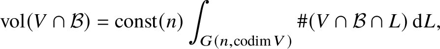 $$ \begin{align} \operatorname{vol}(V\cap{\mathcal B}) = \operatorname{const}(n) \int_{G\left(n,\operatorname{codim} V\right)} \#(V\cap{\mathcal B}\cap L) \,\mathrm d L, \end{align} $$
where  $G(n,k)$ denotes the space of all k-dimensional linear subspaces of
  ${\mathbb C}^{n}$ with the standard measure.
We now pass to general position with respect to V, as in Section 4.2. Since our reparametrising map can be assumed to be close to the identity, this does not change the volume by a factor of more than (say)  $2$. Hence it is enough to estimate the volume in the new coordinates, and by equation (57) it will suffice to show that
  $\#(V\cap {\mathcal B}\cap L)$ is appropriately bounded for every
  ${\boldsymbol \xi }$-linear subspace of dimension
  $k=\operatorname {codim} V$. Since the
  ${\mathcal B}\cap L$ are all unit balls in leaves of
  $L_{k}{\mathbb M}$, the result now follows by the inductive application of Theorem 1 (using the fact that
  $L_{k}{\mathbb M}$ has no new unlikely intersections with V).
6 Proof of Theorem 3
We start by developing some general material on interpolation of algebraic points in Weierstrass polydiscs. It is convenient to state these results in the general analytic context without reference to foliated spaces, and we take this viewpoint in Section 6.1. In Section 6.2 we finish the proof of Theorem 3.
6.1 Interpolating algebraic points
Set  $n\in {\mathbb N}$. The asymptotic constants in this section will depend only on n. Let
  $\Delta =\Delta _{\mathbf x}\times \Delta _{\mathbf w}\subset {\mathbb C}^{n}$ be a Weierstrass polydisc for an analytic set
  $X\subset {\mathbb C}^{n}$ of pure dimension m. Set
  $F\in {\mathcal O}\left (\bar \Delta \right )$. Let
  ${\mathcal M}\subset {\mathbb N}^{n}$ be the set
 $$ \begin{align} {\mathcal M} := {\mathbb N}^{m}\times\{0,\dotsc,e(X,\Delta)-1\}^{n-m}. \end{align} $$
We also set  $E:=e(X,\Delta )^{n-m}$. Recall the following result combining [Reference Binyamini and Novikov12, Theorem 3] and [Reference Binyamini and Novikov11, Proposition 8]:
Proposition 24. On  $\Delta ^{2}$ there is a decomposition
 $$ \begin{align} F = \sum_{\alpha\in{\mathcal M}} c_{\alpha} {\mathbf x}^{\alpha} + Q, \quad Q\in{\mathcal O}\left(\Delta^{2}\right), \end{align} $$
where Q vanishes on  $\Delta ^{2}\cap X$ and
 $$ \begin{align} \left\lVert c_{\alpha} {\mathbf x}^{\alpha} \right\rVert_{\Delta^{2}} = O\left(2^{-\lvert\alpha\rvert} \cdot \left\lVert F \right\rVert_{\Delta}\right). \end{align} $$
 We now fix  $\Phi \in {\mathcal O}(\Delta )^{m+1}$. In [Reference Binyamini and Novikov12], Proposition 24 was used in combination with the interpolation determinant method of Bombieri and Pila [Reference Bombieri and Pila17] to produce an algebraic hypersurface interpolating the points of
  $X\cap \Delta ^{2}$ where
  $\Phi $ takes algebraic values of a given height in a fixed number field. However, this method does not produce good bounds when one considers the more general
  $\left [X\cap \Delta ^{2}\right ](g,h;\Phi )$, where the number field may vary. Instead, we will use an alternative approach proposed by Wilkie [Reference Wilkie53], which is based on the following variant of the Thue–Siegel lemma. This idea was used in a slightly different context by Habegger in [Reference Habegger29].
Lemma 25 [Reference Waldschmidt51, Lemma 4.11]
Set  $A\in \operatorname {Mat}_{\mu \times \nu }({\mathbb R})$. For any
  $N\in {\mathbb N}$, there exists a vector
  ${\mathbf v}\in {\mathbb Z}^{\nu }\setminus \{0\}$ satisfying
 $$ \begin{align} \begin{aligned} \left\lVert {\mathbf v} \right\rVert_{\infty}\le N+1, \qquad \left\lVert A{\mathbf v} \right\rVert_{\infty} \le N^{\frac{\mu-\nu}\mu} \left\lVert A \right\rVert_{\infty}. \end{aligned} \end{align} $$
By combining Proposition 24 and Lemma 25, we obtain the following:
Lemma 26. Set  $d,N\in {\mathbb N}$. There exists a polynomial
  $P\in {\mathbb Z}[y_{1},\dotsc ,y_{m+1}]\setminus \{0\}$ with
  $\deg P\le d$ and all coefficients bounded in absolute value by N, such that
 $$ \begin{align} \left\lVert (P\circ\Phi){\vert_{X\cap\Delta^{2}}} \right\rVert \le \operatorname{poly}(d) E \left\lVert \Phi \right\rVert_{\Delta}^{d} (N \log N) 2^{-d\left(E^{-1}\log N\right)^{\frac1{m+1}}}. \end{align} $$
Proof. Let  $\Phi ^{\alpha }$ for
  $\alpha \in {\mathbb N}^{m+1}$ denote the monomial in the
  $\Phi $ variables with the usual multiindex notation. Note that
  $\left \lVert \Phi ^{\alpha } \right \rVert \le \left \lVert \Phi \right \rVert ^{\lvert \alpha \rvert }$. For each
  $\lvert \alpha \rvert \le d$, apply Proposition 24 to
  $\Phi ^{\alpha }$ to get
 $$ \begin{align} \Phi^{\alpha} = \sum_{\beta\in{\mathcal M}} c_{\alpha,\beta} {\mathbf x}^{\beta} + Q, \quad Q\in{\mathcal O}\left(\Delta^{2}\right), \end{align} $$
where Q vanishes on  $\Delta ^{2}\cap X$ and
 $$ \begin{align} \left\lVert c_{\alpha,\beta} {\mathbf x}^{\beta} \right\rVert_{\Delta^{2}} = O\left(2^{-\lvert\beta\rvert} \cdot \left\lVert \Phi \right\rVert_{\Delta}^{d}\right). \end{align} $$
 Fix  $k\in {\mathbb N}$ to be chosen later. Using Lemma 25, we find a linear combination
  $\sum _{\lvert \alpha \rvert \le d}v_{\alpha } \Phi ^{\alpha }$ with
  $v_{\alpha }$ integers and
  $\lvert v_{\alpha }\rvert <N$, not all zero, such that for every
  $\lvert \beta \rvert \le k$ we have
 $$ \begin{align} \left\lVert \sum_{\lvert\alpha\rvert\le d} v_{\alpha} c_{\alpha,\beta}x^{\beta} \right\rVert_{\Delta^{2}} = O\left(\left\lVert \Phi \right\rVert_{\Delta}^{d}\right)\cdot N^{\frac{\mu-\nu}\mu}, \quad \mu \sim E k^{m}, \ \nu \sim d^{m+1}. \end{align} $$
We now write
 $$ \begin{align} \sum_{\lvert\alpha\rvert\le d} v_{\alpha} \Phi^{\alpha} = \sum_{\lvert\beta\rvert\le k}\sum_{\lvert\alpha\rvert\le d} v_{\alpha} c_{\alpha,\beta}x^{\beta} +\sum_{\lvert\beta\rvert>k} \sum_{\lvert\alpha\rvert\le d} v_{\alpha} c_{\alpha,\beta}x^{\beta} =A+B. \end{align} $$
For A we have by equation (65) the estimate
 $$ \begin{align} A \le O\left(E k^{m} \left\lVert \Phi \right\rVert_{\Delta}^{d}\right)\cdot N^{\frac{\mu-\nu}\mu}, \end{align} $$
and for B we have by equation (64) the estimate
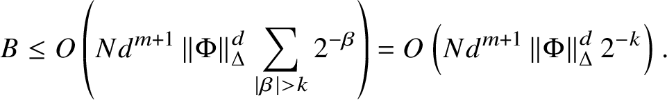 $$ \begin{align} B \le O\left(N d^{m+1} \left\lVert \Phi \right\rVert_{\Delta}^{d} \sum_{\lvert\beta\rvert>k} 2^{-\beta}\right) = O\left(N d^{m+1}\left\lVert \Phi \right\rVert_{\Delta}^{d}2^{-k}\right). \end{align} $$
Choosing  $k=d\left (E^{-1}\log N\right )^{1/(m+1)}$ proves the lemma.
We will compare the upper bound of Lemma 26 with the following elementary lower bound at points where  $\Phi $ takes algebraic values of bounded height and degree:
Lemma 27 [Reference Habegger29, Lemma 14]
Let  $P\in {\mathbb Z}[y_{1},\dotsc ,y_{m+1}]$ be a polynomial of degree d and all coefficients bounded in absolute value by N. Suppose that
  ${\mathbf y}\in \left ({\mathbb Q}^{\mathrm {alg}}\right )^{m+1}$ and
  $P({\mathbf y})\neq 0$. Then
 $$ \begin{align} \lvert P({\mathbf y})\rvert \ge \left(d^{m+1} N H({\mathbf y})^{d(m+1)}\right)^{-[{\mathbb Q}({\mathbf y}):{\mathbb Q}]}. \end{align} $$
 For a subset  $A\subset {\mathbb C}^{n}$, we denote
 $$ \begin{align} A(g,h;\Phi) := \{ p\in A : [{\mathbb Q}(\Phi(p)):{\mathbb Q}] \le g \text{ and } h(\Phi(p))\le h\}. \end{align} $$
We now come to our interpolation result.
Proposition 28. The set  $\left [\Delta ^{2}\cap X\right ](g,h;\Phi )$ is contained in the zero locus of
  $P\circ \Phi $, where
  $P\in {\mathbb Z}[y_{1},\dotsc ,y_{m+1}]\setminus \{0\}$ and
 $$ \begin{align} \deg P\sim g\cdot E\cdot \left(gh+\log\left\lVert \Phi \right\rVert_{\Delta}\right)^{m}, \qquad h(P) \sim E\cdot\left(gh+\log\left\lVert \Phi \right\rVert_{\Delta}\right)^{m+1}. \end{align} $$
Proof. Set  $d,N\in {\mathbb N}$ and construct the polynomial P as in Lemma 26. At any point
  ${\mathbf x}\in \left [\Delta ^{2}\cap X\right ](g,h;\Phi )$, if
  $P\circ \Phi (x)\neq 0$, then
 $$ \begin{align} \left[\operatorname{poly}(d)\cdot N \cdot 2^{(m+1)hd}\right]^{-g} \le \lvert P\circ\Phi({\mathbf x})\rvert \le \operatorname{poly}(d) E \left\lVert \Phi \right\rVert_{\Delta}^{d} (N \log N) 2^{-d\left(E^{-1}\log N\right)^{\frac1{m+1}}}, \end{align} $$
and hence
 $$ \begin{align} 2^{-O\left(\frac{g \log N}d + gh +\log\left\lVert \Phi \right\rVert_{\Delta}+\frac{\log E}d\right)} \le 2^{-\left(E^{-1} \log N\right)^{\frac1{m+1}}}. \end{align} $$
Now choose
 $$ \begin{align} d&=C^{m+1}E \left(gh+\log\left\lVert \Phi \right\rVert_{\Delta}\right)^{m}\cdot g, \end{align} $$
 $$ \begin{align} \log N&=C^{m+1}E\left(gh+\log\left\lVert \Phi \right\rVert_{\Delta}\right)^{m+1}. \end{align} $$
Then formula (73) becomes
 $$ \begin{align} 2^{-O\left(gh +\log\left\lVert \Phi \right\rVert_{\Delta}\right)} \le 2^{-C\left(gh +\log\left\lVert \Phi \right\rVert_{\Delta}\right)}, \end{align} $$
which is impossible for a sufficiently large constant  $C=C(m)$, and we deduce that
  $P\circ \Phi $ vanishes on
  $\left [\Delta ^{2}\cap X\right ](g,h;\Phi )$, as claimed.
6.2 Finishing the proof of Theorem 3
Theorem 3 follows immediately from the following inductive step, where we start with  ${\mathcal W}={\mathbb C}^{\ell }$ and proceed until
  $\operatorname {dist}({\mathcal B},\Sigma (V,{\mathcal W}))<\varepsilon $:
Proposition 29. Let  ${\mathcal W}\subset {\mathbb C}^{\ell }$ be an irreducible
  ${\mathbb Q}$-variety of positive dimension. Suppose that
  $\varepsilon :=\operatorname {dist}({\mathcal B},\Sigma (V,W))$ is positive. Then there exists a collection of irreducible
  ${\mathbb Q}$-subvarieties
  $\{{\mathcal W}_{\alpha }\subset {\mathcal W}\}$ of codimension
  $1$ such that
 $$ \begin{align} {\mathcal W}\cap A(g,h) \subset \cup_{\alpha} {\mathcal W}_{\alpha} \end{align} $$
and
 $$ \begin{align} \#\{{\mathcal W}_{\alpha}\}, \max_{\alpha} \delta_{{\mathcal W}_{\alpha}} = \operatorname{poly}\left(\delta_{\boldsymbol\xi},\delta_{V},\delta_{\mathcal W},\delta_{\Phi},g,h,\log \varepsilon^{-1}\right). \end{align} $$
Proof of Proposition 29
Define  $m:=\dim {\mathcal W}$. Set
  $V^{\prime }=V\cap \Phi ^{-1}({\mathcal W})$. We claim that
 $$ \begin{align} \left\{ p: \dim\left(V^{\prime}\cap{\mathcal L}_{p}\right)\ge m \right\} \subset \Sigma(V,{\mathcal W};\Phi). \end{align} $$
Indeed, if  $p\not \in \Sigma (V,{\mathcal W};\Phi )$, then
  $\Phi _{V\cap {\mathcal L}_{p}}$ is finite. If
  $V^{\prime }\cap {\mathcal L}_{p}$ has a component C of dimension at least m, then
  $\dim \Phi (C)\ge m$ and
  $C\subset {\mathcal W}$, so
  $\Phi (C)$ is a component of
  ${\mathcal W}$ – contradicting the definition of
  $\Sigma (V,{\mathcal W};\Phi )$.
Using Proposition 22, we find a complete intersection W of codimension  $n-m+1$ containing
  $V^{\prime }$ and satisfying
  $\Sigma _{W}\subset \Sigma (V,{\mathcal W};\Phi )$ with appropriate control over
  $\delta _{W}$. Using Theorem 2, we cover
  ${\mathcal B}^{2}$ by sets
  $\Delta _{\beta }^{2}$, where
  $\Delta _{\beta }$ is a Weierstrass polydisc for
  ${\mathcal B}\cap W$ and
  $\#\left \{\Delta _{\beta }\right \}$ and
  $e\left ({\mathcal B}\cap W,\Delta _{\beta }\right )$ are bounded as in equation (78).
Choose a set of m coordinates  $S\subset \{1,\dotsc ,\ell \}$ such that the projection of
  ${\mathcal W}$ to these coordinates is dominant. Using Proposition 28 we construct a polynomial
  $P_{\beta }\in {\mathbb Z}[y_{1},\dotsc ,y_{\ell }]\setminus \{0\}$ depending only on the variables
  $\{y_{s}\}_{s\in S}$ such that
  $\delta (P_{S})=\operatorname {poly}(g,h,\delta _{\Phi })$ and
  $P_{\beta }\circ \Phi $ vanishes identically on
  $\left [\Delta _{\beta }^{2}\cap W\right ](g,h;\Phi )$. Finally, taking
  $\{{\mathcal W}_{\alpha }\}$ to be the union of the collection of irreducible components of
  ${\mathcal W}\cap \left \{P_{\beta }=0\right \}$ for every
  $\beta $ proves the claim.
7 Diophantine applications
Theorem 3 gives, under suitable conditions, an effective polylogarithmic version of the counting theorem of Pila and Wilkie [Reference Pila and Wilkie47]. The counting theorem has found numerous applications in various problems of Diophantine geometry, and our principal motivation in pursuing Theorem 3 is the potential for effectivising these applications. In this section we illustrate how this can be achieved for two of the influential applications: Masser and Zannier’s finiteness result for simultaneous torsion points on elliptic squares [Reference Masser and Zannier38] and Pila’s proof of the André–Oort conjecture for modular curves [Reference Pila45]. Each of these directions has led to significant progress and numerous additional results, many of which seem to be amenable to the same ideas. We also prove a Galois-orbit lower bound for torsion points on elliptic curves, following an idea of Schmidt. We focus on the most basic examples in each of these directions to present the method in the simplest context; we will address some of the more involved applications separately in the future.
7.1 Simultaneous torsion points
Let  $T\subset {\mathbb C}^{4}\times ({\mathbb C}\setminus \{0,1\})$ denote the fibred product of two copies of the Legendre family,
 $$ \begin{align} T = \left\{(x_{1},y_{1},x_{2},y_{2},\lambda) : y_{j}^{2}=x_{j}\left(x_{j}-1\right)\left(x_{j}-\lambda\right), j=1,2\right\}. \end{align} $$
The fibre of T over  $\lambda $ is an elliptic square
  $E_{\lambda }\times E_{\lambda }$, and we use the additive notation for the group law on this scheme. We will also write
  $P=(x_{1},y_{1})$ and
  $Q=(x_{2},y_{2})$.
Theorem 6. Let  $C\subset T$ be an irreducible curve over a number field
  ${\mathbb K}$ with nonconstant
  $\lambda $. Suppose that no relation
  $nP=mQ$ holds identically on C, for any
  $(n,m)\in {\mathbb N}^{2}\setminus \{0\}$. Then at any point
  $c\in C$ where
  $P(c),Q(c)$ are both torsion, their corresponding orders of torsion are effectively bounded by
  $\operatorname {poly}(\delta _{C},[{\mathbb K}:{\mathbb Q}])$.
The proof is given in Section 8. This theorem implies finiteness of the set of simultaneous torsion points, which is the main statement of [Reference Masser and Zannier38]. It also implies that the set of simultaneous torsion points is effectively computable in polynomial time: for each possible torsion order k up to the bound provided in the theorem, one can compute the algebraic equations  $\left (P^{k},Q^{k},c\right )=(\infty ,\infty ,c)$ using the group law on T, intersect with the equation defining
  $C\subset T$ and use elimination theory or Gröbner-basis algorithms to compute the sets of solutions c.
We remark that numerous variations on the theme of Theorem 6 have been studied by Masser and Zannier [Reference Masser and Zannier41, Reference Masser and Zannier37, Reference Masser and Zannier39, Reference Masser and Zannier40], Barroero and Capuano [Reference Barroero and Capuano4, Reference Barroero and Capuano2, Reference Barroero and Capuano3] and Schmidt [Reference Schmidt49]. These include very interesting applications to the solvability of Pell’s equation in polynomials and to integrability in elementary terms. Effective bounds for these contexts, analogous to Theorem 6, should in principle provide the last step toward effective solvability of these classical problems. While we do not address these generalisations directly in this paper, they do appear to be similarly amenable to our methods. We have developed some of the material (most specifically the growth estimates in Appendix A) with an eye to treating the more general types of period maps arising in these applications.
7.2 André–Oort for modular curves
We refer the reader to [Reference Pila45] for the general terminology related to the André–Oort conjecture in the context of  ${\mathbb C}^{n}$. We will prove the following:
Theorem 7. Let  $V\subset {\mathbb C}^{n}$ be an algebraic variety over a number field
  ${\mathbb K}$. Then the degrees of all maximal special subvarieties, as well as the discriminants of all their special coordinates, are bounded by
  $\operatorname {poly}_{n}(\delta _{V},[{\mathbb K}:{\mathbb Q}])$. Here the implied constant is not effective. Moreover, there exists an algorithm that computes the collection of all maximal special subvarieties of V in
  $\operatorname {poly}_{n}(\delta _{V},[{\mathbb K}:{\mathbb Q}])$ steps.
The proof is given in Section 9. Note that this is the only point in this paper where the implied asymptotic constant is not effectively computable in principle. The constants depend on Siegel’s asymptotic lower bound for class numbers, and obtaining an effective form of this bound is a well-known and deep problem. The effectivity of this universal constant notwithstanding, Theorem 7 still establishes the polynomial-time decidability of the André–Oort conjecture in  ${\mathbb C}^{n}$ for fixed n. We also note that the constants do depend effectively on n, so the result also establishes the decidability of the conjecture for
  ${\mathbb C}^{n}$ with n considered as a variable. We remark that the André–Oort conjecture for more general products of modular curves can be proved by reduction to the
  ${\mathbb C}^{n}$ case, and this certainly preserves effectivity, but we do not pursue the details of this here.
7.3 A Galois-orbit lower bound for torsion points
We will prove the following:
Theorem 8. Let E be an elliptic curve defined over a number field  ${\mathbb K}$, and
  $p\in A$ a torsion point of order n. Then
 $$ \begin{align} n=\operatorname{poly}_{g}([{\mathbb K}:{\mathbb Q}],h_{\mathrm{Fal}}(E),[{\mathbb K}(p):{\mathbb K}]). \end{align} $$
The proof is given in Section 10. This theorem is not new: it follows (with more precise dependence on the parameters) from the work of David [Reference David22]. It has also been generalised to abelian varieties of arbitrary genus under some mild conditions [Reference David21] (see also [Reference Masser and Zannier41] for the general case). The proof presented here is different, replacing the use of transcendence methods by point counting using an idea of Schmidt.
We restrict our formal presentation to the elliptic case, as the general case requires some additional technical tools that we do not treat in this paper. However, we sketch in Section 10.4 how the proof extends to arbitrary genus (we restrict to principally polarised abelian varieties, and do not consider the general case). We also mention further implications for Galois-orbit lower bounds in Shimura varieties in Section 10.2.
8 Proof of Theorem 6
To simplify our presentation, we will assume everywhere that  ${\mathbb K}={\mathbb Q}$, but the proof is essentially the same in the general case.
8.1 The foliation
We will construct a one-dimensional foliation encoding for each  $c\in C$ a pair of lattice generators
  $(f,g)$ for the curve
  $E_{\lambda (c)}$ and a pair of elliptic logarithms
  $z,w$ for the points
  $P(c),Q(c)\in E_{\lambda (c)}$. This can be done with the help of the classical Picard–Fuchs differential operator as follows.
We will work in the space over  ${\mathbb C}$ given by
 $$ \begin{align} {\mathbb M} := C\times G, \quad G:=(\operatorname{Mat}_{2\times2},+)\rtimes(\operatorname{GL}_{2},\cdot), \end{align} $$
where we use the matrix  $M_{L}$ (resp.,
  $M_{P}$) to denote the coordinate on the second (resp., third) factor, and more specifically write
 $$ \begin{align} M_{L} = \begin{pmatrix} z & w \\ \dot z & \dot w \end{pmatrix}, \qquad M_{P} = \begin{pmatrix} f & g \\ \dot f & \dot g \end{pmatrix}. \end{align} $$
We consider G as a semidirect product with respect to the left action of  $\operatorname {GL}_{2}$ on
  $\operatorname {Mat}_{2\times 2}$ given by
  $M_{P}\cdot M_{L}=M_{P} M_{L}$ – that is, with the product rule
 $$ \begin{align} (M_{L},M_{P})\left(M_{L}^{\prime},M_{P}^{\prime}\right) = \left(M_{L}+M_{P} M_{L}^{\prime},M_{P} M_{P}^{\prime}\right). \end{align} $$
 Let  $\Sigma \subset {\mathbb C}_{\lambda }$ denote the set consisting of
  $0,1$, the critical values of
  $\lambda {\vert _{C}}$ and the points where
  $\lambda =x_{1}(\lambda )$ or
  $\lambda =x_{2}(\lambda )$ (compare [Reference Masser and Zannier38, p. 459], where a similar choice is made). We set
  $A_{\lambda }={\mathbb C}\setminus \Sigma $ and replace C by the part of C that lives over
  $A_{\lambda }$.
We will take our foliation  ${\mathcal F}$ to be generated by a vector field
 $$ \begin{align} \xi := \tfrac{\partial}{\partial\lambda} + \tfrac{\partial x_{1}}{\partial\lambda}\tfrac{\partial}{\partial x_{1}}+\dotsb+\tfrac{\partial\dot w}{\partial\lambda}\tfrac{\partial}{\partial\dot w}, \end{align} $$
and will show how to express each of the  $\tfrac {\partial }{\partial \lambda }$-derivatives of the coordinates as regular functions on
  ${\mathbb M}$.
We start with the coordinates of C. Since we assume  $\lambda {\vert _{C}}$ is submersive, there is a unique lift of
  $\tfrac {\partial }{\partial \lambda }$, thought of as a section of
  $T(A_{\lambda })$, to a section
  $\xi _{C}$ of
  $T(C)$. The coordinates of this section are regular functions, and their height and degree can be readily estimated, for example, by writing out
  $T(C)$ explicitly as a Zariski tangent bundle. The
  $\tfrac {\partial }{\partial x_{j}}$- and
  $\tfrac {\partial }{\partial y_{j}}$-coordinates of
  $\xi _{C}$ give our
  $\tfrac {\partial x_{j}}{\partial \lambda }$ and
  $\tfrac {\partial y_{j}}{\partial \lambda }$.
We now turn to the equations for  $(f,g)$. Recall that each elliptic period
 $$ \begin{align} I(\lambda) := \oint_{\delta(\lambda)}\omega, \quad \omega=\frac{\,\mathrm d x}y, \end{align} $$
where  $\delta (\lambda )\in H_{1}(E_{\lambda })$ is a continuous family, satisfies the Picard–Fuchs equation
 $$ \begin{align} L I(\lambda)=0, \quad L=\lambda(1-\lambda)\tfrac{\partial^{2}}{\partial\lambda^{2}}+(1-2\lambda)\tfrac{\partial}{\partial\lambda}-\frac14. \end{align} $$
We encode the fact that f satisfies this second-order equation by requiring
 $$ \begin{align} \tfrac{\partial}{\partial\lambda} f = \dot f, \qquad \tfrac{\partial}{\partial\lambda} \dot f = \frac{(1/4)f - (1-2\lambda)\dot f}{\lambda(1-\lambda)}. \end{align} $$
Note that  $\lambda (1-\lambda )$ is invertible on
  $A_{\lambda }$. We impose the same equations on
  $(g,\dot g)$.
Finally, to handle  $z,w$, recall that each elliptic logarithm
 $$ \begin{align} \hat I(\lambda) := \int_{\infty}^{P(\lambda)} \omega \end{align} $$
satisfies an inhomogeneous Picard–Fuchs equation. More explicitly, applying the operator L to  $\hat I(\lambda )$, we obtain by direct computation
 $$ \begin{align} L\hat I(\lambda) = B+\int_{\infty}^{P(\lambda)} L \omega =B+\int_{\infty}^{P(\lambda)} \frac12 \,\mathrm d\left(\frac{y}{(x-\lambda)^{2}}\right) = B+\frac12 \frac{y_{1}(\lambda)}{(x_{1}(\lambda)-\lambda)^{2}}, \end{align} $$
where B denotes the terms coming from the derivation of the boundary points – for example,  $\omega (P(\lambda )^{\prime })$ for the first derivative. To make this computation explicitly, write
  $y:=\sqrt {x(x-1)(x-\lambda )}$ as a function of
  $x,\lambda $, express the integral as a path integral in the x-plane and use the usual derivation rules.
Denote the right-hand side of equation (90) by  $R_{z}$. Then
  $R_{z}$ is a regular function on
  ${\mathbb M}$ by our definition of
  $A_{\lambda }$, and the explicit derivation readily shows that
  $\delta _{R}=\operatorname {poly}(\delta _{C})$. We may thus write the equations for z as
 $$ \begin{align} \tfrac{\partial}{\partial\lambda} z = \dot z, \qquad \tfrac{\partial}{\partial\lambda} \dot z = \frac{(1/4)z - (1-2\lambda)\dot z+R_{z}}{\lambda(1-\lambda)}. \end{align} $$
We impose a similar set of equations on  $(w,\dot w)$, with the right-hand side
  $R_{w}$.
As a consequence of this construction, one leaf  ${\mathcal L}_{0}$ of our foliation is given (locally) by the graph over C of
  $(f,g,z,w)$, where
  $f,g$ are taken to be the two generators of the lattice
  $E_{\lambda }$ and
  $z,w$ are taken to be elliptic logarithms of
  $P(\lambda ),Q(\lambda )$. As one analytically continues, this leaf
  ${\mathcal L}_{0}$ obtains other choices for the generators
  $f,g$ and the logarithms
  $z,w$.
We will also require a description of the remaining leaves. This is fairly simple to obtain: our equations for  $f,g$ are equivalent to the Gauss–Manin linear equations
  $Lf=Lg=0$. For the standard leaf
  ${\mathcal L}_{0}$, these are taken to be two linearly independent solutions, and any other solution is obtained by replacing
  $M_{P}$ with
  $M_{P}G_{P}$ for some
  $G_{P}\in \operatorname {GL}_{2}({\mathbb C})$. Similarly, the equations for
  $z,w$ are equivalent to
  $Lz=R_{z},Lw=R_{w}$, and since
  $f,g$ form a basis of solutions of the homogeneous equations on any leaf, any other leaf with the same
  $f,g$ is obtained by replacing
  $M_{L}$ with
  $M_{L}+M_{P}G_{L}$ for some
  $G_{L}\in \operatorname {Mat}_{2\times 2}({\mathbb C})$. In other words,
  ${\mathcal F}$ is a flat structure of the principal G-bundle
  ${\mathbb M}$, where G acts on itself by multiplication on the right.
8.2 Degree and height bounds
We need two lemmas from [Reference Masser and Zannier38] on the degree and height of points  $c\in C$ where either P or Q is torsion.
Lemma 30 [Reference Masser and Zannier38, Lemma 7.1]
Let  $c\in C$ be such that
  $P(c)$ or
  $Q(c)$ is torsion of order n. Then
 $$ \begin{align} n \le \operatorname{poly}(\delta_{C},[{\mathbb Q}(\lambda(c)):{\mathbb Q}],h(\lambda(c))). \end{align} $$
Proof. This follows at once from the proof of [Reference Masser and Zannier38, Lemma 7.1], where one just needs to track down the constant c to find that it is  $c=\delta _{C}$. We also give an independent proof in Section 10.
Lemma 31 [Reference Masser and Zannier38, Lemma 8.1]
Let  $c\in C$ be such that
  $P(c)$ or
  $Q(c)$ is torsion. Then
 $$ \begin{align} h(\lambda(c)) \le \operatorname{poly}(\delta_{C}). \end{align} $$
Proof. Without the explicit dependence on  $\delta _{C}$, this is [Reference Masser and Zannier38, Lemma 8.1]. The dependence on
  $\delta _{C}$ can be seen from the proof of [Reference Zannier and Masser55, Proposition 3.1]. Specifically, it comes down to Zimmer’s estimate for the difference between the Néron–Tate height
  $\hat h(P)$ and Weil height
  $h(P)$ in the function field case, where the explicit form given in [Reference Zimmer56, p. 40, Theorem] shows that the asymptotic constants are
  $\operatorname {poly}(\delta _{C})$.
Recall that we defined  $A_{\lambda }:={\mathbb C}\setminus \Sigma $ for some finite set
  $\Sigma $. For
  $\delta>0$, we define
  $\Lambda _{\delta }\subset A_{\lambda }$ as
 $$ \begin{align} \Lambda_{\delta} := \left\{ \lambda : \lvert\lambda\rvert<\delta^{-1},\ \forall\sigma\in\Sigma: \lvert\lambda-\sigma\rvert>\delta \right\}. \end{align} $$
We record a consequence of Lemma 31.
Lemma 32 [Reference Masser and Zannier38, Lemma 8.2]
Set  $\lambda \in A_{\lambda }$. Then for
  $\delta =2^{-\operatorname {poly}\left (\delta _{C},h(\lambda )\right )}$, at least half of the Galois conjugates of
  $\lambda $ are in
  $\Lambda _{\delta }$.
Proof. The proof is the same as [Reference Masser and Zannier38, Lemma 8.2]. Briefly, we have an upper bound on the heights of  $\lambda $ and
  $\lambda -\sigma $ for
  $\sigma \in \Sigma $, and this means that averaging over the Galois orbit, none of these can be too small (or too big) in absolute value.
8.3 Setting up the domain for counting
Let  $c\in C$ be such that
  $P(c),Q(c)$ are both torsion, and let n denote the maximum among their orders of torsion and
  $N(c):=[{\mathbb Q}(c):{\mathbb Q}]$. According to Lemma 31, we have
  $h(\lambda (c))=\operatorname {poly}(\delta _{C})$. Then by Lemma 32, at least half of the Galois orbit of
  $\lambda (c)$ lies in a set
  $\Lambda _{\delta }$ with some
  $\delta =2^{-\operatorname {poly}\left (\delta _{C}\right )}$. Moreover,
 $$ \begin{align} n=\operatorname{poly}(\delta_{C},N(c)) \end{align} $$
by Lemma 30.
We choose a collection of  $\operatorname {poly}(\delta _{C})$ discs
  $D_{i}\subset A_{\lambda }$ such that
 $$ \begin{align} D_{i}^{1/4}\subset\Lambda_{\delta/2}, \quad \Lambda_{\delta}\subset\cup_{i} D_{i}. \end{align} $$
This is possible by elementary plane geometry using a logarithmic subdivision process. For example, it is enough to show that for each  $r>0$, one can make such a choice of discs
  $D_{i}$ with
  $D_{i}^{1/4}\subset \Lambda _{r/2}$ to cover
  $\Lambda _{r}\setminus \Lambda _{2r}$. This is equivalent, after rescaling by r, to proving the same fact for
  $r=1$, and here the number of discs
  $D_{i}$ is easily seen to depend polynomially on the number of points in
  $\Sigma $.
In conclusion, we have proved the following:
Lemma 33. There exists one disc  $D=D_{i}$ and one branch of the curve C over
  $D_{i}$ such that the number of Galois conjugates
  $c_{\sigma }$ with
  $\lambda (c_{\sigma })\in D_{i}$ and
  $(P(c_{\sigma }),Q(c_{\sigma }))$ in the chosen branch of C is at least
  $N(c)/\operatorname {poly}(\delta _{C})$.
8.4 Growth estimates for the leaf
We will consider the ball  ${\mathcal B}$ in
  ${\mathcal L}_{0}$ corresponding to
  $D^{1/2}$ in the
  $\lambda $-coordinate, with the
  $P,Q$ coordinates corresponding to the branch of C chosen in Lemma 33. To apply Theorem 3 we must estimate the radius of the ball
  ${\mathbb B}_{R}$ containing this leaf. This can possibly be done by hand for the elliptic case treated in this paper, but we give a more general approach using growth estimates for differential equations which seems easier to carry out in more general settings.
Remark 34. The main difficulty is in obtaining appropriate estimates for the elliptic logarithms  $z,w$. These are given by incomplete elliptic integrals. In the early examples considered by Masser and Zannier, these endpoints were taken to have constant x-coordinates, say
  $x=2,3$. In such cases the incomplete integrals can be estimated in a straightforward manner.
When one considers an arbitrary curve C, the integration endpoints vary with  $c\in C$. It is then necessary to carefully choose the integration path to avoid passing near singularities, and to track how the integration path is deformed as one analytically continues over a domain in C. In general, throughout such a deformation the length of the integration path may unavoidably grow as it picks up copies of vanishing cycles by the Picard–Lefschetz formula. Effectively controlling this phenomenon in terms of the degree and height of C already appears fairly difficult to do by hand.
We start with the coordinates  $P,Q$. Since
 $$ \begin{align} \log \operatorname{dist}^{-1}\left(D^{1/2},\Sigma\right) = \operatorname{poly}(\delta_{C}), \end{align} $$
one can check that the coordinates  $P,Q$ are bounded by
  $e^{\operatorname {poly}\left (\delta _{C}\right )}$. For instance, one may use the general effective bounds for semialgebraic sets proved in [Reference Basu and Roy5], though for this special case much more elementary arguments would suffice. We proceed to consider the remaining coordinates, which are given by (transcendental) elliptic integrals and require a more delicate approach.
Consider first the elliptic periods  $f,g$. Fix some
  $\lambda _{0}\in {\mathbb C}\setminus \{0,1\}$, say
  $\lambda _{0}=1/2$. For some fixed choice of the integration paths staying away from
  $0,1,\lambda _{0},\infty $, we can directly estimate
 $$ \begin{align} \lvert f\rvert,\left\lvert\dot f\right\rvert,\lvert g\rvert,\left\lvert\dot g\right\rvert,\frac1{\operatorname{Im}(f/g)} < M_{0} \end{align} $$
at  $\lambda =\lambda _{0}$ with
  $M_{0}$ an effective constant. Indeed, for such a path the integrals are nicely convergent, and one can approximate them up to any given precision effectively and find such a constant. Our goal is to deduce an effective estimate for these quantities after analytic continuation from
  $\lambda _{0}$ to
  $D^{1/2}$.
Recall that  $f,g$ satisfy the Picard–Fuchs differential equation (87). Since this is a Fuchsian equation, the theorem of Fuchs [Reference Ilyashenko and Yakovenko31, Theorem 19.20] implies that
  $f,g$ (and their derivatives) grow polynomially as one approaches the singular locus of the operator (here
  $\lambda =0,1,\infty $) along geodesic lines on
  ${\mathbb P}^{1}$. In Appendix A we prove an effective version of this theorem. Specifically, using Theorem 9 we get for any
  $\lambda \in D^{1/2}$ the estimate
 $$ \begin{align} \lvert f\rvert,\left\lvert\dot f\right\rvert,\lvert g\rvert,\left\lvert\dot g\right\rvert < e^{\operatorname{poly}\left(\delta_{C}\right)}. \end{align} $$
Here we can and do assume, for instance, that we analytically continue the leaf from  $\lambda _{0}$ to
  $D^{1/2}$ along some sequence of discs in
  ${\mathbb P}^{1}$ as explained in the comment following Theorem 9, staying at a distance
  $e^{-\operatorname {poly}\left (\delta _{C}\right )}$ from the singularities. We absorb
  $M_{0}$ in the asymptotic notation.
The estimate for  $\operatorname {Im} (f/g)$ requires a different argument. The ratio of periods
  $f/g$ defines a map
  $D_{i}^{1/4}\to {\mathbb H}$, and by the Schwarz–Pick lemma we have
 $$ \begin{align} \operatorname{diam}_{H}\left( (f/g)\left(D^{1/2}_{i}\right) \right) \le \operatorname{diam}_{D^{1/4}_{i}} D^{1/2}_{i} = \operatorname{const}. \end{align} $$
Thus as we continue from  $\lambda _{0}$ to
  $D^{1/2}$ along a finite sequence of discs
  $D_{i}$ the ratio
  $f/g$ varies by at most
  $\operatorname {poly}(\delta _{C})$ in
  ${\mathbb H}$. In particular,
  $\operatorname {Im}^{-1}(f/g)<e^{\operatorname {poly}\left (\delta _{C}\right )}$ in
  $D^{1/2}$.
The proof for the elliptic logarithms  $z,w$ is similar to that for
  $f,g$. At the origin
  $\lambda _{1}$ of D, we choose
  $z,w$ to be given by an integral (89) with some standard choice of the path far from
  $0,1,\lambda _{1}$. Then as before, we can estimate
  $\lvert z\rvert ,\left \lvert \dot z\right \rvert ,\lvert w\rvert ,\left \lvert \dot w\right \rvert $ at
  $\lambda _{1}$ by
  $e^{\operatorname {poly}\left (\delta _{C}\right )}$. Our goal is to prove the same in
  $D^{1/2}$. Recall that
  $z,w$ satisfy a nonhomogeneous Picard–Fuchs equation (90). Here the right-hand side consists of the regular functions
  $R_{z},R_{w}$ on
  $A_{\lambda }$, which can be estimated from above by
  $\operatorname {poly}\left (\operatorname {dist}^{-1}(\lambda ,\Sigma )\right )$ in the same way as estimating the branches
  $P,Q$. Now using Theorem 9 again gives
 $$ \begin{align} \lvert z\rvert,\left\lvert\dot z\right\rvert,\lvert w\rvert,\left\lvert\dot w\right\rvert < e^{\operatorname{poly}\left(\delta_{C}\right)}. \end{align} $$
To conclude, we have the following:
Lemma 35. For any  $\lambda \in D^{1/2}$, we have effective estimates
 $$ \begin{align} \lvert f\rvert,\left\lvert\dot f\right\rvert,\lvert g\rvert,\left\lvert\dot g\right\rvert,\lvert z\rvert,\left\lvert\dot z\right\rvert,\lvert w\rvert,\left\lvert\dot w\right\rvert,\frac1{\operatorname{Im}(f/g)} \le e^{\operatorname{poly}\left(\delta_{C}\right)}. \end{align} $$
In other words, the ball  ${\mathcal B}$ constructed earlier is contained in
  ${\mathbb M}_{R}$ for
  $\log R=\operatorname {poly}(\delta _{C})$.
8.5 Setting up the counting
We will be interested in counting representations of  $z,w$ as rational combinations of
  $f,g$. For this it will be convenient to expand our ambient space and foliation. Define
 $$ \begin{align} \hat{\mathbb M} := {\mathbb M} \times \operatorname{Mat}_{2\times2}({\mathbb C})_{U}, \end{align} $$
where U denotes the coordinate on the second factor in matrix form. We define the foliation  $\hat {\mathcal F}$ on
  $\hat {\mathbb M}$ as the product of the foliation
  ${\mathcal F}$ on
  ${\mathbb M}$ with the full-dimensional foliation on the second factor (i.e., where a single leaf is the entire space). We will work with a ball
  $\hat {\mathcal B}$ of radius
  $\hat R$ contained in
  $\hat {\mathbb B}_{\hat R}$, where
  $\hat R$ will be suitably chosen later.
Consider the subvariety  $V\subset \hat {\mathbb M}$ given by
 $$ \begin{align} V := \{ (z,w) = (f,g) U \}. \end{align} $$
Note that we do not restrict the entries of U to  ${\mathbb R}$, as this would not be covered by Theorem 3. Let
  $\hat {\mathcal L}_{0}$ denote the lifting of the standard leaf to
  $\hat {\mathbb M}$. We will apply Theorem 3 with
  $\Phi :=U$. Let G act on
  $\operatorname {Mat}_{2\times 2}({\mathbb C})_{U}$ on the right by the formula
 $$ \begin{align} U\cdot(G_{L},G_{P}) = G_{P}^{-1}(U+G_{L}). \end{align} $$
Then the diagonal action on  $\hat {\mathbb M}$ restricts to an action of G on V, and the map
  $\Phi $ is of course G-equivariant. We use this to deduce two functional transcendence statements for all leaves from the corresponding statements for the standard leaf.
Lemma 36. The map  $\Phi {\vert _{\hat {\mathcal L}_{p}\cap V}}$ is finite for any
  $p\in \hat {\mathbb M}$.
Proof. If the map is not finite, then there is some  $U_{0}$ whose fibre, that is, the set
 $$ \begin{align} \{\lambda\in A_{\lambda} : (z(\lambda),w(\lambda))=(f(\lambda),g(\lambda))U_{0}\}, \end{align} $$
is locally of dimension  $1$. For the standard leaf
  $\hat {\mathcal L}_{0}$ this contradicts the functional transcendence lemma [Reference Masser and Zannier38, Lemma 5.1], as it implies that
  $z,w$ are algebraic over
  $f,g$. Since all other leaves are obtained by the G-action, and
  $\Phi $ is equivariant, the same follows for all other leaves.
Lemma 37. Let  ${\mathcal W}\subset {\mathbb C}^{4}$ be a positive-dimensional algebraic block such that
  $\Sigma (V,{\mathcal W})$ meets a ball
  ${\mathcal B}\subset \hat {\mathcal L}_{0}$. Then
  ${\mathcal W}$ is contained in the affine linear space defined by
 $$ \begin{align} (z(\lambda_{0}),w(\lambda_{0})) = (f(\lambda_{0}),g(\lambda_{0})) U \end{align} $$
for some  $\lambda _{0}\in \lambda ({\mathcal B})$.
Proof. This is again just a reformulation of the functional transcendence results from [Reference Masser and Zannier38]. Suppose  ${\mathcal W}$ is not contained in such an affine linear space. Then
  $\Phi \left (\hat {\mathcal L}_{0}\cap V\right )$ contains one of the analytic components of (some germ of)
  ${\mathcal W}$, and in particular
  $\lambda $ is nonconstant on
  $\hat {\mathcal L}_{0}\cap V$ (otherwise this germ would satisfy equation (107) for the constant value
  $\lambda _{0}$). We may also assume without loss of generality that
  ${\mathcal W}$ is a curve by replacing it with its generic section (
 $\lambda $ remains nonconstant for a generic section). Then equation (107) implies that
  $f(\lambda ),g(\lambda )$ have transcendence degree at most
  $1$ over
  $z(\lambda ),w(\lambda )$, contradicting [Reference Masser and Zannier38, Lemma 5.1].
We remark that Lemma 37 implies, in particular, that any block coming from the standard leaf can contain at most one real point: it is a product of two affine linear spaces with complex angle  $(f(\lambda _{0}):g(\lambda _{0}))$. By G-equivariance, the blocks coming from other leaves are obtained as G-translates. For a sufficiently nearby leaf – that is, a G-translate sufficiently close to the origin – the angle is still complex. All such nearby blocks therefore also contain at most one real point. This will be crucial later in our application of Theorem 3.
8.6 Finishing the proof
We fix  $\varepsilon =e^{-\operatorname {poly}\left (\delta _{C}\right )}$, to be suitably chosen later. Apply Theorem 3 to the ball
  $\hat {\mathcal B}$ with
  $V,\Phi $ constructed in Section 8.5. Recall that by Lemma 35 the ball
  ${\mathcal B}$ is contained in a ball of radius
  $e^{\operatorname {poly}\left (\delta _{C}\right )}$ in
  ${\mathbb M}$. The same lemma also shows that
  $\operatorname {Im}(f/g)\ge e^{-\operatorname {poly}\left (\delta _{C}\right )}$ uniformly on
  ${\mathcal B}$. We choose
  $\varepsilon $ small enough so that, by Lemma 37, any block coming from a leaf of distance
  $\varepsilon $ to
  ${\mathcal B}$ is still a product of affine spaces with complex angle (and in particular contains at most one real point). Setting
  $A:={\mathbb R}^{2}\cap \Phi \left (\hat {\mathcal B}^{2}\cap V\right )$, we have
 $$ \begin{align} \# A(1,h) = \operatorname{poly}\left(\delta_{C},\hat R,h\right). \end{align} $$
On the other hand we have the following:
Lemma 38. For suitably chosen  $\hat R = e^{\operatorname {poly}\left (\delta _{C}\right )}$, each Galois conjugate
  $c_{\sigma }$ in Lemma 33 corresponds to a
  ${\mathbb Q}$-rational point of log-height
  $\operatorname {poly}(\delta _{C},\log n)$ in A.
Proof. Recall that  $P(c),Q(c)$ are both torsion of order at most n, and the same is therefore true for each
  $c_{\sigma }$. In the equation
 $$ \begin{align} (z,w) = (f,g) U \end{align} $$
with real U, each  $c_{\sigma }$ corresponds to a single value of U, with all coordinates rational and denominators not exceeding n. The claim follows once we prove that the entries of U are bounded from above by
  $e^{\operatorname {poly}\left (\delta _{C}\right )}$. This follows from Lemma 35. Indeed, we have, for example,
 $$ \begin{align} z = f u_{11} + g u_{12}, \end{align} $$
which can be interpreted as a pair of  ${\mathbb R}$-linear equations on
  $u_{11},u_{12}$ by taking real and imaginary parts. The determinant of this system is at least
  $e^{-\operatorname {poly}\left (\delta _{C}\right )}$, because
  $\operatorname {Im}(f/g)$ is at least
  $e^{-\operatorname {poly}\left (\delta _{C}\right )}$, and the bounds on U follow easily.
In fact, the proof of Theorem 3 gives a bound  $\operatorname {poly}(\delta _{C},h)$ not only for
  $\#A(1,h)$ but for the number of different points
  $\lambda \in D$ corresponding to points in A. A reader having forgotten the proof of Theorem 3 may instead appeal to Corollary 2, which shows that the number of different values of
  $\lambda $ corresponding to a single point of A is at most
  $\operatorname {poly}(\delta _{C},h)$. Indeed, for any fixed value
  $U=U_{0}$ in A, apply the corollary to the set
 $$ \begin{align} {\mathcal B}^{2}\cap V\cap\{U=U_{0}\}, \end{align} $$
using Lemma 36 to see that  $\Sigma $ is empty in this case. It is in fact a simple exercise to remove the dependence on h in this bound, but as we do not need this, we leave it for the reader.
We are now ready to finish the proof. Recall that in Lemma 33 the number of points  $c_{\sigma }$ is at least
  $N(c)/\operatorname {poly}(\delta _{C})$. Thus with
  $h=\operatorname {poly}(\delta _{C},\log n)$, we have
 $$ \begin{align} N(c)/\operatorname{poly}(\delta_{C}) \le \#A(1,h) \le \operatorname{poly}(\delta_{C},\log n)=\operatorname{poly}(\delta_{C},\log N(c)), \end{align} $$
where the last estimate is by equation (95). This immediately implies  $N(c)=\operatorname {poly}(\delta _{C})$, as claimed.
9 Proof of Theorem 7
9.1 The foliation
We follow Pila’s proof [Reference Pila45], which uses the uniformisation of modular curves by the j-function  $j:\Omega \to {\mathbb C}$, where
  $\Omega \subset {\mathbb H}$ denotes the standard fundamental domain for the
  $\operatorname {SL}_{2}({\mathbb Z})$-action. To apply Theorem 3, we encode this graph as a leaf of an algebraic foliation. This could be done by replacing
  $j:{\mathbb H}\to {\mathbb C}$ with the
  $\lambda $-function
  $\lambda :{\mathbb H}\to {\mathbb C}$ and expressing the inverse
  $\tau :{\mathbb C}\to {\mathbb H}$ as the ratio of two elliptic integrals, which satisfy a Picard–Fuchs differential equation as discussed in Section 8.1. For variation here we use an alternative approach, expressing j directly as a solution of a Schwarzian-type differential equation (which was used for a similar purpose in [Reference Binyamini8]).
Recall that the Schwarzian operator is defined by
 $$ \begin{align} S(f) = \left(\frac{f^{\prime\prime}}{f^{\prime}}\right)^{\prime} - \frac12 \left(\frac{f^{\prime\prime}}{f^{\prime}}\right)^{2}. \end{align} $$
We introduce the differential operator
 $$ \begin{align} \chi(f) = S(f) + R(f) (f^{\prime})^{2}, \quad R(f) = \frac{f^{2}-1968f+2,654,208}{2f^{2}(f-1728)^{2}}, \end{align} $$
which is a third-order algebraic differential operator vanishing on Klein’s j-invariant j [Reference Masser33, p. 20]. As observed in [Reference Freitag and Scanlon24], it easy to check that the solutions of  $\chi (f)=0$ are exactly the functions of the form
  $j_{g}(\tau ):=j\left (g^{-1}\cdot \tau \right )$ where
  $g\in \operatorname {PGL}_{2}({\mathbb C})$ acts on
  ${\mathbb C}$ in the standard manner.
The differential equation may be written in the form  $f^{\prime \prime \prime }=A(f,f^{\prime },f^{\prime \prime })$, where A is a rational function. More explicitly, consider the ambient space
  $M:={\mathbb C}\times {\mathbb C}^{3}\setminus \Sigma $ with coordinates
  $(\tau ,y,\dot y,\ddot y)$, where
  $\Sigma $ consists of the zero loci of
  $y,y-1728$ and
  $\dot y$. In particular, we will write
  ${\mathbb C}_{y}:={\mathbb C}\setminus \{0,1728\}$. On M, the vector field
 $$ \begin{align} \xi := \tfrac{\partial}{\partial\tau} + \dot y \tfrac{\partial}{\partial y} + \ddot y\tfrac{\partial}{\partial\dot y}+A(y,\dot y,\ddot y)\tfrac{\partial}{\partial\ddot y} \end{align} $$
encodes the differential equation, in the sense that any trajectory is given by the graph of a function  $j_{g}(\tau )$ and its first two derivatives.
We define our n-dimensional foliation  ${\mathcal F}$ on the ambient space
  ${\mathbb M}:=M^{n}$ by taking an n-fold cartesian product of M with its one-dimensional foliation determined by the vector field
  $\xi $. We let
  ${\mathcal L}$ denote the standard leaf given by the product of the graphs of the j function, and note that any other leaf is obtained as a product of graphs of
 $$ \begin{align} (j(g_{1}\tau_{1}),\dotsc,j(g_{n}\tau_{n})), \quad (g_{1},\dotsc,g_{n})\in\operatorname{GL}_{2}({\mathbb C})^{n}. \end{align} $$
In fact, one may easily check that  ${\mathcal F}$ is invariant under an appropriate algebraic action of
  $\operatorname {GL}_{2}({\mathbb C})^{n}$, where the action is trivial on y and is computed by the chain rule on
  $\dot y,\ddot y$.
9.2 Reduction to maximal special points
Denote by  $V^{\mathrm {ws}}$ the weakly special locus of V – that is, the union of all weakly special subvarieties of V. In [Reference Binyamini8, Theorem 4] it is shown that one can effectively compute
  $V^{\mathrm {ws}}$, and in particular
  $\delta (V^{\mathrm {ws}})=\operatorname {poly}_{n}(\delta _{V})$. It is also shown that as a consequence of this, one can reduce the problem of computing all maximal special subvarieties to the problem of computing all special points
  $p\in V_{\alpha }\setminus V_{\alpha }^{\mathrm {ws}}$, for some auxiliary collection of varieties
  $V_{\alpha }\subset {\mathbb C}^{n_{\alpha }}$ with
  $n_{\alpha }\le n$ and
  $\sum _{\alpha } \delta (V_{\alpha })=\operatorname {poly}_{n}(\delta _{V})$.
We remark that even though in [Reference Binyamini8] only the bounds on the number and degrees of these auxiliary subvarieties are explicitly stated, the construction in fact yields an effective algorithm, as can be observed directly from the proof. We also note that the proof itself relies on differential algebraic constructions, though of a very different nature than in the present paper. In conclusion, it will suffice to prove Theorem 7 only for special points outside  $V^{\mathrm {ws}}$.
9.3 A bound for maximal special points
We will use Theorem 3 to count maximal special points in V as a function of the discriminant. Toward this end, we define  $\hat V:=\pi _{y}^{-1}(V)\subset {\mathbb M}$, where
  $\pi _{y}:{\mathbb M}\to {\mathbb C}_{y}^{n}$ is the projection to the coordinates
  $(y_{1},\dotsc ,y_{n})$. We let
  $\Phi =(\tau _{1},\dotsc ,\tau _{n})$. Note that
  $\Phi $ restricts to the germ of a finite map locally at every
  ${\mathcal L}_{p}$.
The following proposition will allow us to control the blocks coming from nearby leaves. We denote by  $J:{\mathbb H}^{n}\to {\mathbb C}^{n}$ the n-fold product of the j-function.
Proposition 39. Let  ${\mathcal B}$ be a
  $\xi $-ball in the standard leaf and
  ${\mathcal W}$ a positive- dimensional algebraic block coming from a nearby leaf at distance
  $\varepsilon $. Then
 $$ \begin{align} J({\mathcal W}\cap\pi_{\tau}({\mathcal B})) \subset N_{\delta}(V^{\mathrm{ws}}), \quad \delta=O_{\mathcal B}(\varepsilon), \end{align} $$
where  $N_{\delta }(V^{\mathrm {ws}})$ denotes the
  $\delta $-neighbourhood of
  $V^{\mathrm {ws}}$ with respect to the Euclidean metric on
  ${\mathbb C}^{n}$.
Proof. If  ${\mathcal W}$ comes from the standard leaf, then the modular Ax–Lindemann theorem established in [Reference Pila45] shows that
  ${\mathcal W}$ is contained in a pre–weakly special subvariety
  ${\mathcal W}^{\prime }$ with
  ${\mathcal W}^{\prime }\cap {\mathbb H}^{n}\subset J^{-1}(V)$. More accurately, some branch of a germ of
  ${\mathcal W}$ is contained in
  ${\mathcal W}^{\prime }$, but since
  ${\mathcal W}$ is irreducible, in fact
  ${\mathcal W}\subset {\mathcal W}^{\prime }$. Thus
  $J({\mathcal W}\cap {\mathbb H}^{n})\subset V^{\mathrm {ws}}$ by definition.
Recall that by formula (116), all other leaves are obtained by a  $g\in \operatorname {GL}_{2}({\mathbb C})^{n}$-translate of the standard leaf. A tubular neighbourhood of
  ${\mathcal B}$ of radius
  $\varepsilon $ is thus generated by translates with
  $\left \lVert \operatorname {id}-g \right \rVert =O_{\mathcal B}(\varepsilon )$. If
  ${\mathcal W}$ comes from a leaf in this neighbourhood, then we have by the foregoing argument
 $$ \begin{align} J\left(g^{-1}({\mathcal W}\cap{\mathbb H}^{n})\right)\subset V^{\mathrm{ws}}. \end{align} $$
To finish, we should show that
 $$ \begin{align} J({\mathcal W}\cap\pi_{\tau}({\mathcal B})) \subset N_{O_{\mathcal B}(\varepsilon)}\left(J\left(g^{-1}({\mathcal W}\cap{\mathbb H}^{n})\right)\right). \end{align} $$
This follows at once because  ${\mathcal B}$ is precompact. First,
  ${\mathcal W}\cap \pi _{\tau }({\mathcal B})$ is contained in a neighbourhood of
  $g^{-1}({\mathcal W}\cap {\mathbb H}^{n})$, since the derivative of the G-action is bounded in
  $\pi _{\tau }({\mathcal B})\subset {\mathbb H}^{n}$. And then
  $J({\mathcal W}\cap \pi _{\tau }({\mathcal B}))$ is contained in a neighbourhood of
  $J\left (g^{-1}({\mathcal W}\cap {\mathbb H}^{n})\right )$, since the derivative of J is bounded in
  $\pi _{\tau }({\mathcal B})$.
Let  $p\in V\setminus V^{\mathrm {ws}}$ be a special point. We associate to p the complexity measure
 $$ \begin{align} \Delta(p) := \sum_{i=1}^{n} \lvert\operatorname{disc}(p_{i})\rvert, \end{align} $$
where  $\operatorname {disc} p_{i}$ is the discriminant of the endomorphism ring of the elliptic curve corresponding to
  $p_{i}$. The Chowla–Selberg formula combined with standard estimates on L-functions imply
 $$ \begin{align} h(p) = O_{\varepsilon}(\Delta(p)^{\varepsilon}), \quad \text{for any }\varepsilon>0 \end{align} $$
(see, e.g., [Reference Habegger28, Lemma 4.1] and the estimate for the logarithmic derivative of the L-function in [Reference Tsimerman50, Corollary 3.3]).
Lemma 40. For any  $\varepsilon>0$ and special point
  $p\in V\setminus V^{\mathrm {ws}}$,
 $$ \begin{align} \log \operatorname{dist}^{-1} (p_{\sigma},V^{\mathrm{ws}}) = \operatorname{poly}_{n}(\delta_{V}) O_{\varepsilon}(\Delta(p)^{\varepsilon}) \end{align} $$
holds for at least two-thirds of the Galois conjugates  $p_{\sigma }$ of p.
Proof. This follows from  $\delta (V^{\mathrm {ws}})=\operatorname {poly}_{n}(\delta _{W})$ and equation (121). For instance, choose a polynomial P with
  $h(P)=\operatorname {poly}_{n}(\delta _{V})$ vanishing on
  $V^{\mathrm {ws}}$ but not on p. Then
  $h(P(p))=\operatorname {poly}_{n}(\delta _{V},h(p))$, and in particular for two-thirds of the conjugates
  $p_{\sigma }$ we have
 $$ \begin{align} -\log \lvert p_{\sigma}\rvert=O_{\varepsilon}(\Delta(p)^{\varepsilon}), \qquad -\log \left\lvert P(p_{\sigma}) \right\rvert &= \operatorname{poly}_{n}(\delta_{V},O_{\varepsilon}(\Delta(p)^{\varepsilon})). \end{align} $$
On the other hand, for these conjugates if  $d_{\sigma }:=\operatorname {dist} (p_{\sigma },V^{\mathrm {ws}})$, then by the mean value theorem (assuming, e.g.,
  $d_{\sigma }<1$),
 $$ \begin{align} \left\lvert P(p_{\sigma}) \right\rvert \le \,\mathrm d_{\sigma}\cdot \max_{B_{p_{\sigma}}\left(d_{\sigma}\right)} \left\lVert \,\mathrm d P \right\rVert =e^{\operatorname{poly}_{n}\left(\delta_{V},\Delta(p)^{\varepsilon}\right)} \cdot d_{\sigma}. \end{align} $$
Taking logs and comparing the last two estimates implies equation (122) on  $d_{\sigma }$.
Let  $K\subset \Omega ^{n}\subset {\mathbb H}^{n}$ be a compact subset of the fundamental domain
  $\Omega ^{n}$ with
 $$ \begin{align} \operatorname{vol}(K) \ge \frac23 \operatorname{vol}(\Omega^{n}). \end{align} $$
According to Duke’s equidistribution theorem [Reference Duke23], for  $\lvert \operatorname {disc}(p)\rvert \gg 1$ at least two-thirds of the conjugates
  $p_{\sigma }$ correspond to points in K. Thus at least one-third of the conjugates
  $p_{\sigma }$ both lie in K and satisfy Lemma 40. Call such conjugates good conjugates.
Remark 41. Rather than appealing to equidistribution, it is also possible to use the height estimate (121) to deduce that a large portion of the orbit lies at log-distance at least  $\Delta ^{\varepsilon }$ from the cusp. One can then use a logarithmic subdivision process to cover all such points by
  $\Delta ^{\varepsilon }$-many
  ${\boldsymbol \xi }$-balls, similar to the approach we use in Section 8.3. We use such an approach in [Reference Binyamini, Schmidt and Yafaev15] (with Schmidt and Yafaev) in the context of general Shimura varieties, where the analogous equidistribution statements are not known.
According to Brauer-Siegel [Reference Brauer18], the number of good conjugates is at least
 $$ \begin{align} \frac13 [{\mathbb Q}(p):{\mathbb Q}] \ge \Delta(p)^{c} \quad \text{for some }c>0. \end{align} $$
We also recall from [Reference Pila45] that for each  $p_{\sigma }$, the corresponding preimage
  $\tau _{\sigma }\in \Omega ^{n}$ satisfies
 $$ \begin{align} [{\mathbb Q}(\tau_{\sigma}):{\mathbb Q}] \le 2n, \qquad H(\tau_{\sigma}) = \operatorname{poly}_{n}(\Delta(p)). \end{align} $$
We are now ready to finish the proof. Cover the part of  ${\mathcal L}$ corresponding to K by finitely many unit balls
  ${\mathcal B}\subset {\mathcal L}$ and apply Theorem 3 with
  $\varepsilon _{0}$ to each of them. We choose
 $$ \begin{align} \log \varepsilon_{0}^{-1} = \operatorname{poly}_{n}(\delta_{V}) O_{\varepsilon}(\Delta(p)^{\varepsilon}) \end{align} $$
corresponding to the bound in Lemma 40, so that for any good conjugate  $p_{\sigma }$ the
  $\varepsilon _{0}$-neighbourhood of
  $p_{\sigma }$ does not meet
  $V^{\mathrm {ws}}$. Then according to Corollary 39, none of the positive-dimensional blocks
  ${\mathcal W}_{\alpha }$ coming from nearby leaves at a distance
  $\varepsilon _{0}$ can contain the corresponding
  $\tau _{\sigma }$. Counting with
  $g=2n$ and
  $e^{h}=\operatorname {poly}_{n}(\Delta (p))$, we see that each good conjugate must come from a zero-dimensional
  ${\mathcal W}_{\alpha }$, and the number of good conjugates is therefore
  $\operatorname {poly}_{n}(\delta _{V},O_{\varepsilon }(\Delta (p)^{\varepsilon }))$. Choosing
  $\varepsilon $ sufficiently small compared to c and comparing this to formula (126), we conclude that
  $\Delta (p)<\operatorname {poly}_{n}(\delta _{V})$.
9.4 Computation of the maximal special points
To compute the finite list of maximal special points  $p\in V\setminus V^{\mathrm {ws}}$, we start by enumerating all CM-points
  $p\in {\mathbb C}^{n}$ up to a given
  $\Delta =\delta _{V}$ (in polynomial time). For example, they are all obtained as images under
  $\pi $ of points
  $\tau $ in
  ${\mathbb H}^{n}$, whose coordinates are each imaginary quadratic with height
  $\operatorname {poly}_{n}(\Delta )$. It is simple to enumerate all such points; call them
  $\left \{\tau _{j}\right \}$.
For each  $\tau _{j}$ and each equation
  $P_{k}=0$ defining V, we should check whether
  $P_{k}\left (\pi \left (\tau _{j}\right )\right )$ vanishes. Since
  $\delta _{\pi \left (\tau _{j}\right )}=\operatorname {poly}_{n}(\Delta )$, we have
 $$ \begin{align} \delta\left(P_{k}\left(\pi\left(\tau_{j}\right)\right)\right) = \operatorname{poly}_{n}(\Delta,\delta_{V})=\operatorname{poly}_{n}(\delta_{V}), \end{align} $$
and by Liouville’s inequality, either  $P_{k}\left (\pi \left (\tau _{j}\right )\right )=0$ or
 $$ \begin{align} -\log \left\lvert P_{k}\left(\pi\left(\tau_{j}\right)\right)\right\rvert = \operatorname{poly}_{n}(\delta_{V}), \end{align} $$
so it is enough to compute  $\operatorname {poly}_{n}(\delta _{V})$ bits of
  $P_{k}\left (\pi \left (\tau _{j}\right )\right )$ to check whether it vanishes. This can be accomplished, for instance, by computing with the q-expansion of
  $j(\cdot )$, and we leave the details for the reader.
10 Proof of degree bounds for torsion points
10.1 Schmidt’s strategy
Our proof of Theorem 8 is based on an idea by Schmidt [Reference Schmidt48], who noticed that a polylogarithmic point-counting result such as the one obtained in Theorem 3 would allow one to deduce degree bounds for special points from suitable height bounds (in various contexts). The idea (in the context of an abelian variety A) is to count points on the graph of the universal cover  $\pi :{\mathbb C}^{g}\to A$. If P is an n-torsion point on A, then one has a collection
  $P,P^{2},\dotsc ,P^{n}$ of torsion points. On the graph of
  $\pi $ these correspond to pairs
  $\left (z_{j},P^{j}\right )$ where
  $h\left (P^{j}\right )$ is bounded (as these are torsion points),
  $h\left (z_{j}\right )=O(\log n)$ (where we represent
  $z_{j}$ as combinations of the periods) and
  $P^{j}$ all lie in the field
  ${\mathbb K}(P)$. By point counting, we therefore find
 $$ \begin{align} n = \operatorname{poly}_{A}(\log n,[{\mathbb K}(P):{\mathbb K}]), \end{align} $$
from which the Galois-orbit lower bound follows.
Most applications of the Pila–Wilkie counting theorem use point counting to deduce an upper bound on the size of Galois orbits of special points, contrasting them with lower bounds obtained by other methods (usually transcendence techniques). Schmidt’s idea shows that polylogarithmic point-counting results already carry enough transcendence information to directly imply Galois-orbit lower bounds, giving ‘purely point-counting’ proofs of unlikely intersection statements (modulo the corresponding height bounds, which are of course specific to the problem at hand). It is also to our knowledge one of the first applications of point counting that requires polylogarithmic, rather than the classical subpolynomial, estimates.
Remark 42. In fact, for this method to work, subpolynomial dependence on the height  $H:=e^{h}$ is sufficient. The crucial asymptotic is to obtain polynomial dependence on the degree g. However, in the interpolation methods used to prove the Pila–Wilkie theorem and related theorems, the dependence on g and h are of the same order. Imitating the proof of the classical Pila–Wilkie theorem would give only a subexponential
  $e^{\varepsilon g}$ bound, which is not sufficient.
10.2 Further implications
Though we consider here the simplest context of elliptic curves and abelian varieties, Schmidt’s idea can be made to work also in the context of special points on Shimura varieties. In [Reference Binyamini, Schmidt and Yafaev15], together with Schmidt and Yafaev we prove that height bounds of the form
 $$ \begin{align} h(p) \ll \operatorname{disc}(p)^{\varepsilon} \quad \text{for any }\varepsilon>0, \end{align} $$
where p is a special point in a Shimura variety and  $\operatorname {disc}(p)$ is the discriminant of the corresponding endomorphism ring, imply Galois-orbit lower bounds
 $$ \begin{align} [{\mathbb Q}(p):{\mathbb Q}] \ge \operatorname{disc}(p)^{c} \quad \text{for some }c>0. \end{align} $$
In the case of the Siegel modular variety  $\mathcal {A}_{g}$, the bound (132) follows from the averaged Colmez formula [Reference Andreatta, Goren, Howard and Pera1, Reference Yuan and Zhang54], and Tsimerman [Reference Tsimerman50] has used these height bounds to establish corresponding Galois-orbit lower bounds. For this implication he uses the Masser–Wüstholz isogeny estimates [Reference Masser and Wüstholz35], another deep ingredient based on transcendence methods. We obtain an alternative proof of Tsimerman’s theorem, avoiding the use of isogeny estimates and replacing them with point counting based on Theorem 3. In particular, our proof applies also in the context of general Shimura varieties, where it establishes the André–Oort conjecture conditional on the height bound (132). This seems to be of interest because to our knowledge, the corresponding isogeny estimates are not known for general Shimura varieties, and it is therefore unclear whether Tsimerman’s approach could be used in this generality.
Remark 43. A few months after [Reference Binyamini, Schmidt and Yafaev15] was posted on arXiv, Pila, Shankar and Tsimerman posted [Reference Pila, Shankar, Tsimerman, Esnault and Groechenig46] in which they establish the height conjecture (132) for arbitrary Shimura varieties. Combined with the Galois-orbit lower bound established in [Reference Binyamini, Schmidt and Yafaev15], this finishes the proof of the André–Oort conjecture for general Shimura varieties.
10.3 Proof of Theorem 8
Write  $E=E_{\lambda }$ in Legendre form and define
 $$ \begin{align} h:=\max(h(\lambda),[{\mathbb K}:{\mathbb Q}]). \end{align} $$
It is known that  $h_{\mathrm {Fal}}(E)=\operatorname {poly}(h)$, so we prove the bound with h instead of the Faltings height. Let
  $\xi _{E}$ denote the translation-invariant vector field on E given by
 $$ \begin{align} \xi_{E} := \left[\tfrac12 x(x-1)(x-\lambda)\right]^{\prime}\partial_{y}+y\partial_{x}. \end{align} $$
Note that this is dual to the standard holomorphic form  $\,\mathrm d x/y$ on E. We will work in the ambient space
  ${\mathbb M}:=E_{x,y}\times {\mathbb C}_{z}$, where the subscripts denote the coordinates used on each factor. We will consider the foliation generated by the vector field
 $$ \begin{align} \xi := \xi_{E}+\partial_{z}. \end{align} $$
Any leaf of  ${\mathcal F}$ is the graph of a covering map
  ${\mathbb C}\to E$, and as usual this forms a principal G-bundle with
  $G=({\mathbb C},+)$ acting on
  ${\mathbb C}_{z}$ by translation.
The main technical issue is to cover a large piece of a leaf by  $\operatorname {poly}(h)$-many
  $\xi $-balls with suitable control on the growth. For this it is convenient to renormalise the time parametrisation of
  $\xi $. Recall that
  $x:E\to {\mathbb P}^{1}$ is ramified over the points
  $\Sigma :=\{0,1,\lambda ,\infty \}$. Fix some
  $\delta =e^{-\operatorname {poly}(h)}$ to be chosen later, and denote by
  $\Lambda _{\delta }$ the complement of the
  $\delta $-neighbourhood of
  $\Sigma $. As in Section 8.3, we can choose a collection of
  $\operatorname {poly}(h)$ discs
  $D_{i}$ such that
 $$ \begin{align} D_{i}^{1/2}\subset\Lambda_{\delta/2}, \qquad \Lambda_{\delta}\subset\cup_{i} D_{i}. \end{align} $$
We consider the reparametrised vector field  $\xi ^{\prime }:=\xi /y$. The
  $\xi ^{\prime }$-ball
  ${\mathcal B}_{i}$ around the centre of
  $D_{i}$ with the same radius corresponds to
  $D_{i}$ in the x-variable and to one of the two y-branches in the y-variable. The z-coordinate is obtained by integrating
  $\,\mathrm d x/y$ over
  $D_{i}$, and since the integrand is bounded by
  $e^{\operatorname {poly}(h)}$, we conclude the following:
Lemma 44. The  $\xi ^{\prime }$-ball
  ${\mathcal B}_{i}$ is contained in
  ${\mathbb B}_{R}$ for suitable
  $R=e^{\operatorname {poly}(h)}$.
Now let  $p\in E$ be an n-torsion point and denote
 $$ \begin{align} N(p) := [{\mathbb K}(p):{\mathbb K}]. \end{align} $$
Then the Néron–Tate height of p vanishes, and by Zimmer [Reference Zimmer56] it follows that the usual Weil height satisfies  $h(p)=\operatorname {poly}(h)$. By the same arguments used to prove Lemma 32, at least half of the Galois conjugates of p over
  ${\mathbb K}$, which are also n-torsion, have an x-coordinate in
  $\Lambda _{\delta }$ with some suitable choice
  $\delta =e^{-\operatorname {poly}(h)}$.
We can apply the same argument to the points  $p^{2},p^{3},\dotsc ,p^{n}$, which are also torsion of order at most n, and which crucially satisfy
  $N\left (p^{j}\right )\le N(p)$, since the product law is defined over
  ${\mathbb K}$. Concluding this discussion, we have the following:
Lemma 45. There exist at least  $n/2$ points
  $p_{i}\in E$ that are torsion of order at most n, have height
  $\operatorname {poly}(h)$, satisfy
  $x(p_{i})\in \Lambda _{\delta }$ and have
  $N(p_{i})\le N(p)$.
At least  $n/\operatorname {poly}(h)$ of these points have x-coordinate belonging to a single disc
  $D_{i}$ and y-coordinate in a fixed branch over
  $D_{i}$.
We will derive a contradiction to the assumption that  $N(p)$ is small by counting the points corresponding to
  $p_{i}$ on the leaf of our foliation. Let
  $\bar \omega _{1},\bar \omega _{2}\in {\mathbb C}$ be the two periods of
  $\,\mathrm d x/y$ on E, with
  $\bar \tau =\bar \omega _{2}/\bar \omega _{1}$ in the standard fundamental domain of
  $\operatorname {SL}_{2}({\mathbb Z})$. It is known that
 $$ \begin{align} \left\lvert\bar\omega_{1}\right\rvert^{\pm1},\left\lvert\bar\omega_{2}\right\rvert^{\pm1}=e^{\operatorname{poly}(h)}, \qquad \left\lvert\bar\tau\right\rvert=\operatorname{poly}(h), \end{align} $$
though even  $\left \lvert \bar \tau \right \rvert =e^{\operatorname {poly}(h)}$ would suffice for our purposes.
We consider the ambient space  $\hat {\mathbb M}:={\mathbb M}\times {\mathbb C}^{2}_{u}\times {\mathbb C}^{2}_{\omega }$ with the foliation
  $\hat {\mathcal F}$ given by the product of
  ${\mathcal F}$ with the generator
  $\xi ^{\prime }$ on
  ${\mathbb M}$, the full-dimensional foliation on
  ${\mathbb C}^{2}_{u}$ and the zero-dimensional foliation on
  ${\mathbb C}^{2}_{\omega }$. Consider the variety
  $V\subset \hat {\mathbb M}$ given by
 $$ \begin{align} V := \{ (x,y,z,u_{1},u_{2}) : z=u_{1}\omega_{1}+ u_{2}\omega_{2} \} \end{align} $$
and the map  $\Phi :=(x,y,u_{1},u_{2})$. A leaf of
  $\hat {\mathcal F}$ is given by fixing a leaf of
  ${\mathcal F}$ and a point
  $(\omega _{1},\omega _{2})\in {\mathbb C}^{2}_{\omega }$. Similar to Lemma 37, we have the following:
Lemma 46. Let  ${\mathcal W}$ be a positive-dimensional algebraic block such that
  $\Sigma (V,{\mathcal W})$ meets some leaf
  $\hat {\mathcal L}$. Then
  $u_{1}\omega _{1}+u_{2} \omega _{2}$ is constant on
  ${\mathcal W}$, where
  $\omega _{1},\omega _{2}$ are the
  $\omega $-values taken on
  $\hat {\mathcal L}$.
Proof. Suppose not. Then  ${\mathcal W}$ would imply an algebraic relation between
  $(x,y)$ and
  $z=u_{1}\omega _{1}+u_{2}\omega _{2}$, which would hold in a neighbourhood of some point
  $(x,y,z)$ on a leaf
  ${\mathcal L}$ of
  ${\mathcal F}$. But
  $(x,y)$ are two elliptic functions of z (on any leaf), and are certainly not algebraic over z.
Recall that  $R=e^{\operatorname {poly}(h)}$ is a constant to be chosen later. Let
  ${\mathcal B}={\mathcal B}_{i}$ be the ball corresponding to the disc
  $D_{i}^{1/2}$ of Lemma 45. We consider the polydisc
  $\hat {\mathcal B}$ given by the product of
  ${\mathcal B}$ in the
  $(x,y,z)$ coordinates, a polydisc of radius R in the
  $u_{1},u_{2}$ coordinates and the fixed
  $\omega _{1,2}=\bar \omega _{1,2}$ in the
  $\omega $-coordinates. From
  $\operatorname {Im}\left (\bar \tau \right )\ge 1/\sqrt {2}$ and equation (139), it follows that choosing suitable
  $\varepsilon $ with
  $\varepsilon ^{-1}=e^{\operatorname {poly}(h)}$, we can ensure that the line
  $z=u_{1}\omega _{1}+u_{2}\omega _{2}$, on any leaf at a distance
  $\varepsilon $ from
  $\hat {\mathcal B}$, has a strictly complex angle and in particular contains at most one real point
  $(u_{1},u_{2})$. From Lemma 46, it follows that any block coming from a leaf of distance
  $\varepsilon $ to
  $\hat {\mathcal B}$ contains at most one real point
  $(u_{1},u_{2})$. Apply Theorem 3. Then setting
  $A:={\mathbb R}^{2}\cap \Phi \left (\hat {\mathcal B}^{2}\cap V\right )$, we have
 $$ \begin{align} \# A(g,t) = \operatorname{poly}(h,g,t). \end{align} $$
On the other hand, we have the following:
Lemma 47. Each of the points  $p_{i}$ of Lemma 45 corresponds to a point of log-height
  $t=\operatorname {poly}(h,\log n)$ and degree at most
  $g=[{\mathbb K}:{\mathbb Q}]\cdot N(p)$ in A.
Proof. For the  $x,y$-coordinates this is the content of Lemma 45. For the
  $u_{1},u_{2}$-coordinates, they are rational with denominators at most n, since
  $p_{i}$ is torsion, z is a lifting of
  $p_{i}$ to
  ${\mathbb C}$ and
  $\bar \omega _{1},\bar \omega _{2}$ generate the lattice of E in the z-coordinate. The numerators are also bounded by
  $e^{\operatorname {poly}(h)}$: for z this bound is given in Lemma 44, and the same bound for
  $u_{1},u_{2}\in {\mathbb R}$ follows since
  $z=u_{1}\bar \omega _{1}+ u_{2}\bar \omega _{2}$ and
  $\operatorname {Im}\left (\bar \omega _{1},\bar \omega _{2}\right )\ge 1/\sqrt 2$ and equation (139) holds. Thus choosing a suitable
  $R=e^{\operatorname {poly}(h)}$, we see that
  $u_{1},u_{2}$ are indeed rational of log-height
  $\operatorname {poly}(\log n,h)$ and in the polydisc of radius R.
Finally, we have
 $$ \begin{align} n/\operatorname{poly}(h) \le \#A(N(p)\cdot[{\mathbb K}:{\mathbb Q}],\operatorname{poly}(h,\log n)) = \operatorname{poly}(h,N(p),\log n), \end{align} $$
and it follows that  $n=\operatorname {poly}(h,N(p))$, as claimed.
10.4 Abelian varieties of arbitrary genus
There is no difficulty in extending the foregoing proof to show that if A is an abelian variety of genus g over  ${\mathbb K}$ and
  $p\in A$ is torsion of order n, then
  $n \le \operatorname {poly}_{A}([{\mathbb K}(p):{\mathbb K}])$. The more technically challenging part is to establish the precise dependence on A, namely
 $$ \begin{align} n = \operatorname{poly}_{g}([{\mathbb K}:{\mathbb Q}],[{\mathbb K}(p):{\mathbb K}],h_{\mathrm{Fal}}(A)). \end{align} $$
We briefly sketch how the argument presented in the elliptic case can be extended to arbitrary genus, assuming that A is principally polarised.
An explicit embedding of A in projective space can be computed in terms of the theta function  $\Theta :A\to {\mathbb P}^{N}$. The theta height of A is defined by
  $h:=h_{\Theta }(A)=h(\Theta (0))$. By [Reference Pazuki43, Corollary 1.3], the Faltings height is roughly the same as the theta height, and we can use this as a replacement of the
  $h(\lambda )$ used in the elliptic case. By, for example, [Reference Masser and Wüstholz36, Lemma 3.1], the image
  $\Theta (A)$ is defined by a collection of quadratic equations whose coefficients are functions of
  $\Theta (0)$; so as in the elliptic case, we have
 $$ \begin{align} h(\Phi(A))=\operatorname{poly}_{g}(h). \end{align} $$
The translation-invariant vector fields  ${\boldsymbol \xi }:=(\xi _{1},\dotsc ,\xi _{g})$ used to construct the foliation can also be explicitly expressed in terms of
  $h(\Theta (0))$ [Reference Masser and Wüstholz36, Lemma 3.7], and in particular
  $\delta _{\boldsymbol \xi }=\operatorname {poly}_{g}(h)$.
The main technical issue is the covering of A by  $\operatorname {poly}_{g}(h)$-many
  ${\boldsymbol \xi }$-balls. (Here if one is content with a general bound depending on A rather than polynomial in h, compactness can be used.) In the elliptic case, we achieved this by explicitly constructing a covering by balls in the x-coordinate. In arbitrary dimension one obviously needs a more systematic approach. For instance, the results of [Reference Binyamini and Novikov13] show that
  $\Theta (A)$ can be covered by
  $\operatorname {const}(g)$ charts whose domains are complex cells. When
  $\Theta (A)$ is further assumed to be of height h, one can in fact replace these general cells by
  $\operatorname {poly}_{g}(h)$ polydiscs (this is a work in progress with Novikov and Zack). Having obtained such a collection of polydiscs replacing our discs
  $D_{i}$ in the elliptic case, one can proceed with the proof without major changes.
A Growth estimates for inhomogeneous Fuchsian equations
A.1 Gronwall for higher-order linear ODEs
Let  $D\subset {\mathbb C}$ be a disc and consider a linear differential operator
 $$ \begin{align} L = a_{0}(t) \partial_{t}^{n}+a_{1}(t)\partial_{t}^{n-1}+\dotsb+a_{n}(t) \end{align} $$
where  $a_{0},\dotsc ,a_{n}$ are holomorphic in
  $\bar D$. Let
  $b(t)$ also be holomorphic in
  $\bar D$. We will consider the growth of solutions for the inhomogeneous equation
 $$ \begin{align} Lf=b(t). \end{align} $$
We denote
 $$ \begin{align} j_{t}^{n}f:=\left(f,\partial_{t}f,\dotsc,\partial_{t}^{n}f\right)^{T}, \qquad v_{b}:=(0,\dotsc,0,b(t))^{T}. \end{align} $$
The following is a form of the Gronwall inequality for monic linear operators:
Lemma 48. Suppose that  $a_{0}\equiv 1$ and denote
 $$ \begin{align} A = \max_{j=1,\dotsc,n}\max_{t\in\bar D} \left\lvert a_{j}(t)\right\rvert, \qquad B = \max_{t\in\bar D} \lvert b(t)\rvert. \end{align} $$
Then for every  $t\in D$,
 $$ \begin{align} \left\lVert j_{t}^{n}f(t) \right\rVert \le e^{O_{n}(A)} \left(O_{n}(B)+\left\lVert j_{t}^{n}f(0) \right\rVert\right). \end{align} $$
Proof. Rewrite  $Lf=b$ as a linear system for the vector
  $j_{n}^{t}f$ as follows:
 $$ \begin{align} \partial_{t} j_{t}^{n}f(t) = \begin{pmatrix} 0 & 1 & 0 & \cdots & 0 \\ 0 & 0 & 1 & \cdots & 0 \\ & & \vdots & & \\ -a_{n}(t) & -a_{n-1}(t) & \cdots & -a_{2}(t) & -a_{1}(t) \end{pmatrix} j_{t}^{n}f(t) &+ v_{b}(t) = \Omega(t)j_{t}^{n}f(t)+v_{b}(t). \end{align} $$
Then for  $t\in D$, the solution
  $j_{t}^{n}f$ satisfies
 $$ \begin{align} \partial_{t} \left\lVert j_{t}^{n}f(t) \right\rVert \le \left\lVert \Omega \right\rVert\cdot\left\lVert j_{t}^{n}f(t) \right\rVert+O_{n}(B) = O_{n}(A)\left\lVert j^{n}f_{t}(t) \right\rVert+O_{n}(B), \end{align} $$
and the conclusion follows by the classical Gronwall inequality.
Lemma 48 allows one to prove growth estimates for general equations  $Lf=b$ nonsingular in a disc D by first dividing by the leading term. However, due to the exponential dependence on A, the resulting bound will grow exponentially as a function of the minimum of the leading term. For arbitrary singular linear ordinary differential equations, this is the best one can expect.
For Fuchsian operators, which are the operators that come up in the study of periods and logarithms, one can obtain much sharper estimates with polynomial growth near the singularities. We do this in the following section.
A.2 Inhomogeneous Fuchsian equations
In this section we assume that the coefficients of L are in  ${\mathbb C}[t]$. Recall that L is called Fuchsian if each singular point
  $t_{0}\in {\mathbb P}^{1}$ of L is Fuchsian. This means that in a local coordinate z where
  $t_{0}$ is the origin, L can be written in the form
 $$ \begin{align} L = \tilde a_{0}(z)(z\partial_{z})^{n}+\tilde a_{1}(z)(z\partial_{z})^{n-1}+\dotsb+\tilde a_{n}(z), \end{align} $$
where the coefficients  $\tilde a_{j}$ are holomorphic at the origin and
  $\tilde a_{0}(0)\neq 0$. We denote by
  $\Sigma \subset {\mathbb P}^{1}$ the set of singular points of L.
We recall the notion of slope for a differential operator over  ${\mathbb C}(t)$ introduced in [Reference Binyamini, Novikov and Yakovenko14]. For a polynomial p, we define
  $\left \lVert p \right \rVert $ to be the
  $\ell _{1}$-norm on the coefficients. We extend this to rational functions by setting
  $\left \lVert p/q \right \rVert =\left \lVert p \right \rVert /\left \lVert q \right \rVert $, where the fraction
  $p/q$ is reduced.
Definition 49 slope of a differential operator
The slope  $\angle L$ of L is defined by
 $$ \begin{align} \angle L := \max_{i=1,\dotsc,n} \frac{\left\lVert a_{j}(t) \right\rVert}{\left\lVert a_{0}(t) \right\rVert}. \end{align} $$
The invariant slope  $\sphericalangle L$ is defined by
 $$ \begin{align} \sphericalangle L := \sup_{\phi\in\operatorname{Aut}\left({\mathbb P}^{1}\right)} \angle (\phi^{*}L), \end{align} $$
where  $\phi ^{*}L$ denotes the pullback of L by
  $\phi $.
We remark that in [Reference Binyamini, Novikov and Yakovenko14] the slope was defined by first normalising the coefficients  $a_{j}$ to be polynomials, but this minor technical difference does not affect what follows. It is a general fact that the invariant slope is finite for Fuchsian operators [Reference Binyamini, Novikov and Yakovenko14, Proposition 32]. The following gives effective estimates when L is defined over a number field
  ${\mathbb K}$. In this case we denote
  $\delta _{L}:=\sum _{j}\delta _{a_{j}}$.
Proposition 50. Suppose L is defined over a number field. Then  $\sphericalangle L=e^{\operatorname {poly}_{n}\left (\delta _{L}\right )}$.
Proof. Since  $\sphericalangle L$ is defined by a semialgebraic formula over a number field and is known to be finite, an effective bound follows from general effective semialgebraic geometry [Reference Basu and Roy5]; see the derivation in [Reference Binyamini, Novikov and Yakovenko14, Section 3.6.2].
The slope  $\sphericalangle L$ is useful for studying the oscillation of solutions of homogeneous Fuchsian equations
  $Lf=0$, and for the study of growth. In the inhomogeneous case we also require the following corollary concerning the leading coefficient. We denote by
  $a_{j}(L)$ the jth coefficient of L.
Proposition 51. Suppose L is defined over a number field. Then
 $$ \begin{align} \inf_{\phi\in\operatorname{Aut}\left({\mathbb P}^{1}\right)} \left\lVert a_{0}(\phi^{*}L) \right\rVert = e^{-\operatorname{poly}_{n}\left(\delta_{L}\right)}. \end{align} $$
Proof. We first prove that the infimum is positive. Assume the contrary. Then we may choose  $\phi $ such that
  $\left \lVert a_{0}(\phi ^{*}L) \right \rVert $ is arbitrarily small. By the boundedness of
  $\sphericalangle L$, this means that
  $\left \lVert a_{j}(\phi ^{*}L) \right \rVert $ is also arbitrarily small. Now the operator
  $L^{\prime }:=L+1$ is also Fuchsian, and
  $\left \lVert a_{0}(\phi ^{*}L^{\prime }) \right \rVert =\left \lVert a_{0}(\phi ^{*}L) \right \rVert $ is arbitrarily small, while
  $\left \lVert a_{n}(\phi ^{*}L^{\prime }) \right \rVert =\left \lVert 1+a_{n}(\phi ^{*}L) \right \rVert $ is arbitrarily close to
  $1$. This contradicts the boundedness of
  $\sphericalangle L^{\prime }$. The effective bound is then obtained in the same way as in Proposition 50.
We will also need the following simple lemma:
Lemma 52. Let r be a rational function and D denote the unit disc. If r has no poles in  $D^{1/2}$, then
 $$ \begin{align} \max_{z\in D}\lvert r(z)\rvert \le e^{O(\deg r)} \left\lVert r \right\rVert, \end{align} $$
and if r has no zeros in  $D^{1/2}$, then
 $$ \begin{align} \min_{z\in D}\lvert r(z)\rvert \ge e^{-O(\deg r)}\left\lVert r \right\rVert. \end{align} $$
Proof. Without loss of generality,  $\left \lVert r \right \rVert =1$. Write
  $r=p/q$ with
  $p,q$ polynomials and
  $\left \lVert p \right \rVert =\left \lVert q \right \rVert =1$. Suppose q has no zeros in
  $D^{1/2}$. Then
 $$ \begin{align} \lvert q(z)\rvert \ge e^{-O(\deg q)} \text{ for every }z\in D, \end{align} $$
by, for example, [Reference Binyamini and Yakovenko16, Lemma 7]. Since  $\lvert p(z)\rvert $ is bounded by
  $1$ for
  $z\in D$, the upper bound on
  $r(z)$ follows. The lower bound follows by repeating for
  $1/r$.
We now come to our main theorem. If  $D=D_{r}(t_{0})$ is a disc, we call
  $z=(t-t_{0})/r$ a natural coordinate on D.
Theorem 9. Let L be a Fuchsian operator as before, defined over a number field. Let  $D=D_{r}(t_{0})$ be a disc with
  $D^{1/2}\subset {\mathbb C}\setminus \Sigma $ and z a natural coordinate on D. Consider the equation
  $Lf=b$, where b is defined in
  $D^{1/2}$ and bounded by B there. Then for
  $t_{1}\in D$,
 $$ \begin{align} \left\lVert j^{n}_{z}f(t_{1}) \right\rVert \le e^{c_{L}} \left(B+\left\lVert j^{n}_{z}f(t_{0}) \right\rVert\right), \quad c_{L}:=e^{\operatorname{poly}_{n}\left(\delta_{L}\right)}. \end{align} $$
In particular,
 $$ \begin{align} \left\lVert j^{n}_{t}f(t_{1}) \right\rVert \le \max(r,1/r)^{n} e^{c_{L}} \left(B+\left\lVert j^{n}_{t}f(t_{0}) \right\rVert\right). \end{align} $$
Proof. Note that  $j^{n}_{z}f$ is obtained from
  $j^{n}_{t}f$ by multiplying the jth coordinate by
  $r^{j}$, so the second estimate follows from the first.
Let  $\hat L$ denote the pullback of L to the z-coordinate and set
  $\hat a_{j}=a_{j}\left (\hat L\right )$. By Propositions 50 and 51, we have
 $$ \begin{align} \angle \hat L, \left\lVert \hat a_{0} \right\rVert^{-1} = e^{\operatorname{poly}\left(\delta_{L}\right)}. \end{align} $$
Dividing by the leading term, we have an equation
 $$ \begin{align} \left(\partial_{z}^{n}+\frac{\hat a_{1}}{\hat a_{0}}\partial_{z}^{n-1}+\dotsb+\frac{\hat a_{n}}{\hat a_{0}}\right)f=b/\hat a_{0}. \end{align} $$
The claim will now follow from Lemma 48, once we establish suitable bounds for the coefficients and for the right-hand side. These bounds follow from equation (161) and Lemma 52 applied to obtain a lower bound for  $\hat a_{0}$ (which has no zeros in
  $D^{1/2}$) and an upper bound for
  $\hat a_{j}$ (which has no poles in
  $D^{1/2}$).
Theorem 9 allows one to obtain a polynomial bound on the growth of solutions for equations  $Lf=b$, assuming b has polynomial growth. To see this, consider a fixed
  $t_{0}\in {\mathbb C}$ and an arbitrary
  $t_{1}\in {\mathbb C}$, say of distance
  $\delta $ to
  $\Sigma $. Connect
  $t_{0}$ to
  $t_{1}$ by a sequence of
  $O(\log \delta )$ discs
  $D_{i}$ with
  $D_{i}^{1/2}\subset {\mathbb C}\setminus \Sigma $, such that the sequence of radii
  $r_{i}$ satisfies, for example,
  $1/2<r_{i}/r_{i+1}<2$. It is a simple exercise in plane geometry to check that this can always be achieved. Then applying Theorem 9 consecutively for the discs
  $D_{i}$ and assuming b is bounded by
  $\operatorname {poly}(1/\delta )$ throughout gives an estimate on the branch of f at
  $t_{1}$ obtained by analytic continuation along the
  $D_{i}$, namely
 $$ \begin{align} f(t_{1}) = \operatorname{poly}_{L}(1/\delta)\left\lVert j^{n}_{t}f(t_{0}) \right\rVert. \end{align} $$
Here one should use the statement in the natural coordinate z, noting that by our assumption on the radii the distortion in jets when switching from coordinate  $z_{i}$ to
  $z_{i+1}$ is bounded by
  $2^{n}$ at each step. If one uses the statement with the t-coordinate, then one gets the slightly larger
  $\delta ^{O(\log \delta )}$ term (which is still suitable for our purposes in this paper).
Remark 53. The geometric requirements on the chains of discs  $D_{i}$ are not arbitrary; they represent an actual obstruction. For instance, consider the function
 $$ \begin{align} f(x) = \sqrt{\varepsilon^{2}+x^{2}}+x. \end{align} $$
As an algebraic function, this satisfies a Fuchsian equation  $L_{\varepsilon } f=0$ with singularities at
  $\{\varepsilon ,-\varepsilon ,\infty \}$. For
  $\varepsilon \ll 1$, one branch of this function becomes uniformly small while the other tends uniformly to
  $2x$. On the other hand, the slope of the operators
  $L_{\varepsilon }$ is uniformly bounded as a function of
  $\varepsilon $, for instance by the results of [Reference Binyamini, Novikov and Yakovenko14] (or by direct computation for this simple case). However, to analytically continue from one of these branches to the other, one must at some point pass between
  $-\varepsilon $ and
  $\varepsilon $. To do this, some of the discs
  $D_{i}$ would have to be of size
  $O(\varepsilon )$, and this explains why one cannot obtain an estimate for one branch in terms of the other branch which is uniform in
  $\varepsilon $.
Acknowledgements
This research was supported by the Israel Science Foundation (grant 1167/17) and by funding received from the MINERVA Stiftung with funds from the BMBF of the Federal Republic of Germany. This project also received funding from the European Research Council under the European Union’s Horizon 2020 research and innovation programme (grant agreement 802107).
Conflict of Interest:
None.


 Open access