

- EAER>
- Journal Archive>
- Contents>
- articleView
Contents
Citation
| No | Title |
|---|---|
| 1 | / 2023 / |
| 2 | High-speed rail construction and urban innovation disparity in China: the role of internet development / 2023 / Economic Change and Restructuring / vol.56, no.5, pp.3567 / |
| 3 | The impact of internet development on green total factor productivity in China’s prefectural cities / 2023 / Information Technology for Development / vol.29, no.4, pp.462 / |
Article View
East Asian Economic Review Vol. 25, No. 1, 2021. pp. 3-31.
DOI https://dx.doi.org/10.11644/KIEP.EAER.2021.25.1.389
Number of citation : 3View
165
Download
131
Benefits and Spillover Effects of Infrastructure: A Spatial Econometric Approach
|
|
Economic Research and Regional Cooperation Department, Asian Development Bank |
|---|---|
|
|
Sustainable Development and Climate Change Department, Asian Development Bank |
|
|
School of Statistics, University of the Philippines |
|
|
Department of Economics, Georgia State University |

Abstract
This paper estimates the effects of transport (road and rail) & energy and ICT infrastructure (telephone, mobile, and broadband) on GDP growths in neighboring countries as well as own countries. We confirm positive direct contributions of infrastructure, access to Internet, and human capital on economic growth. The spatial panel regression models indicate that there exist positive externalities of the broadband infrastructure and human capital, and these results are robust regardless of the choice of spatial weight matrices. Our findings on spillover effects of infrastructure suggest the key role of neighboring countries’ infrastructure on own country’s economic growth.
JEL Classification: C21, D24, D62
Keywords
Infrastructure, Spillover Effects, Economic Growth, Production Function, Spatial Econometrics
I. Introduction
The positive contribution of infrastructure on economic growth has long been found in a large body of the literature, although the magnitude of the impact is the subject of considerable uncertainty. As one of the major production factors, higher infrastructure capital is strongly associated with higher income. Figure 1 indicates strong positive correlation between per capita income and selective proxies for infrastructure capital stock including road, energy, mobile, and broadband. When combined with financially interconnected markets, infrastructure allows people and capital to move more freely not just within own countries but to other countries in the neighborhood that can be defined in terms of geographical or economic proximity, creating spillover effects across borders.
For instance, these intra- and inter-country externalities, in the case of building and enhancing a transport network, are made possible through redistribution of production resources and productivity gains due to agglomeration (Tong et al., 2013). And the transport network enables the impact of the global value chains, a formal source of spillover effects, to more easily extend across multiple economies. At the same time the use of ICT increases productivity internally by raising the quality and productivity of other inputs, and externally by facilitating dissemination of knowledge from one firm, industry, or country to another (Moshiri, 2016). Rising interconnectedness through infrastructure and its externalities suggests that investigating economic benefits of infrastructure should take into account not only direct impacts within a country, but also indirect impacts that propagate over its neighboring countries.
This paper estimates the economic benefits of infrastructure on output. Two broad categories of infrastructure are examined: (1) transport (roads and rails) and energy, and (2) the ICT infrastructure that covers telephone, mobile, and fixed broadband subscriptions. We employ spatial econometric analysis to estimate separately the direct as well as indirect or cross-border benefits of infrastructure.
In our preferred spatial panels models, significant and positive cross-border spillover effects of the broadband infrastructure and human capital are found under the assumption that economic connectivity is represented by physical proximity. These results are robust to the choice of a spatial weight matrix. Our results also indicate that rail infrastructure show positive and significant output impacts on neighboring countries as well as on own countries.
While most studies have employed this method in the analysis of subnational economy spillovers, this paper is one of the few studies that explicitly applies the spatial econometric approach to cross-county infrastructure panel data. The results highlight the need to distinguish the non-infrastructure variable from the total capital stock variable that are commonly used in the empirical models together with infrastructure stock variables that are already included in the estimates of total capital. Our paper also attempts to shed light on the literature on regional public goods (RPGs). RPGs are defined as public goods whose non-excludable and non-rivalry benefits extend beyond a single nation’s territory to some well-defined region (Sandler, 2006). A transportation network is a good example of an RPG. Most literature in this area is theoretical or qualitative, while attempts to measure RPGs are usually limited to the input side or investments in RPGs. Thus, another value-added of this paper is the attempt to measure the output side of RPGs by estimating the direct benefits and spillover effects of infrastructure as an RPG.1
The paper is organized as follows. Section II outlines a brief survey of the literature discussing the benefits and spillover effects of infrastructure, followed by the motivations for the use of the spatial econometric models in achieving this paper’s objectives. Section III explains the structure of the non-spatial and spatial panel models to be estimated. Section IV discusses the data, and Section V presents the results of non-spatial and spatial models. Section VI concludes.
1)It might be more reasonable to limit our focus to cross-border infrastructure given its intended influence on multiple countries targeted. However, cross-country data on cross-border infrastructure are rarely available. Instead, this study uses national level infrastructure data which conceptually covers the infrastructure that connects to other countries. Our approach can be viewed from the perspective that being connected locally is a necessary condition for being connected across borders, thus local infrastructure in place ultimately contributes to higher cross-border connectivity. For the percentage of cross-border (or regional) infrastructure of total infrastructure projects, an indicative measure for Asia points to approximately 4%, which is comparable to Europe
II. Literature Review
1. Benefits and Spillover Effects of Infrastructure
The key role of physical infrastructure is often highlighted in terms of facilitating trade and reducing trade costs in the empirical studies where variants of the gravity models are commonly used. The majority of the infrastructure variables in those studies are perception-based indicators collected from surveys, which makes it difficult to interpret the degrees of their changes by nature.
Several studies confirm the existence of spillover effects of transport and ICT infrastructure on output. These are mostly based on sub-national studies such as in the People’s Republic of China (PRC), and in a few developed countries. For recent examples, exploring cities in Hunan province, PRC, Hu and Luo (2017) find that road infrastructure has a significant positive direct as well as indirect effect on economic growth, with the indirect effect greater than the direct effect. Yu et al. (2013) find the existence of both positive and negative spatial spillovers of infrastructure in the PRC regions. For the US states, Tong et al. (2013) find that road disbursement has a significant positive direct effect on a state’s agricultural output, while also beneficial to agricultural development in other states.
For ICT infrastructure, Moshiri (2016) shows that ICT can have a positive impact on labor productivity, but with differences across regions, industries, and time (Moshiri, 2016).2 The results show that the impact of ICT investment in the US on Canada, a major trading partner, has spilled over to some Canadian provinces and industries while the overall ICT effects are concentrated in those ICT-intensive provinces and industries. ICT capital is also found to be an important source of total factor productivity growth (van Leeuwen and van der Wiel, 2003). More recently, Lin et al. (2017) find the evidence of the spillover effect of the Internet, highlighting its effects on growth as a conduit through which new technology flows to neighboring regions to generate new knowledge and to facilitate the exchange of knowledge.
Spillover effects of infrastructure can also be negative, as found in the literature. An increase in infrastructure in neighboring countries may negatively affect the own region’s economy. While intra-regional effects of infrastructure are generally positive, the negative inter-regional spillover effects can be explained by a competing economic relationship between the own and neighboring regions in acquiring resources for production (while a positive inter-regional spillover means a complementary relationship) or the regions may be competing for markets for the products that they produce. The studies at the subnational level find that infrastructure investment in one region may draw mobile production factors away from other regions (for examples on the US, see Boarnet, 1998; Cohen and Manaco, 2007 and Sloboda and Yao, 2008). Regional competition takes various forms depending on horizontal/vertical competitive relations and the type of competition and competitors (Batey and Friedrich, 2000). In the case of cross-country spillover effects, one can expect smaller degrees of negative (or positive) externalities, if any, given the higher restrictions imposed on factor movements across countries.
2. Motivation for the Use of Spatial Econometric Models
To provide a basis for the use of the spatial econometric methods in achieving the objectives of the paper, we briefly review the following: (1) an omitted variables motivation, (2) spatial heterogeneity motivation, and (3) externalities-based motivation (LeSage and Pace, 2009).
In spatial samples, an omitted variable bias easily arises when unobservable factors (e.g. locational advantages) that are likely to be spatially correlated have an influence on the dependent variable (e.g. national income). A spatial autoregressive (SAR) model can address this omitted variable bias with a spatial lag (i.e. a linear combination of neighbors’ y’s).

where
Unlike a panel regression model with the coefficients assumed to be identical for all observational units, a spatial panel model allows each spatial unit to react differently mainly because each unit has different set of neighbors and is affected by them. This can be easily shown in the reduced form of the SAR model with abs(

where (
As the impact of a shock dissipates over time through a temporal lag in the AR model, the SAR model allows us to model a spatial dependence where a shock in the error at any location is transmitted to other regions, with its impact dissipating over physical or economic distance (Anselin, 2003). Moreover, externalities from neighbors’ characteristics (

2)Unlike transport infrastructure generally measured by the lengths of total roads and rails, the proxies for ICT infrastructure come in various forms due to its wider scope of coverage
III. Model
1. Non-spatial Panel Regression Model
For the non-spatial panel models, the Cobb-Douglas production function is used, following Calderón et al. (2015).


where
2. Spatial Panel Regression Model
(1) Spatial weight matrix3
The economic growth of a country is affected by the characteristics of its neighbors when spatial spillover effects are present. The definition of a neighborhood depends on a symmetric weight matrix, denoted by  all with a 25th percentile cutoff, i.e., the neighbors of a particular country are only the closest 25% of all countries in terms of distance. Countries with distance beyond the cutoff have a weight of zero. The use of a percentile cutoff instead of an absolute distance cutoff reduces the effect of country area size.
(2) Spatial Durbin Model
The spatial Durbin model (SDM) is implemented to account for the spatial spillover effect in the production function of country

where
(3) Average direct and indirect impacts
The expected values of y’s in the SDM can be written in a matrix form:

where 
The average direct effect is given by:

The average total effect is given by:

The average indirect effect is estimated from the difference of the average total effect and the average direct effect.
3)In a spatial weight matrix, the extent to which a location is interconnected with all other locations is imposed a priori. Thus, the spatial weight matrix should not be treated as something to be estimated, but as exogenous. As such, geography-based (e.g. contiguity- and distance-based) weights that are free of the endogeneity issue have been widely used. This paper also follows this traditional concept of a spatial weigh matrix that requires to be exogenous. However, interconnectedness can be represented by economic distance such as trade flows and there have been many attempts to address an endogenous spatial weight matrix in the recent spatial econometrics literature. Authors leave this issue to our future research agenda.
4)This study follows an approach commonly used in the literature to compute the distance between two countries. It is calculated by first plotting the country centroids using a Geographic Information System (GIS) country shapefile, then spherical distance functions were used to compute the distance in kilometers between the centroids.
IV. Data5
The variables were primarily taken from the dataset in Calderón et al. (2015) which spans only from 1960 to 2000 and we extended it up to 2014. Two new ICT infrastructure variables, mobile and fixed broadband subscriptions, were added. In the final dataset, we have a panel data for 78 countries covering years 1960 to 2014 except for mobile and broadband subscriptions that are available from 1995 to 2014.6
The dependent variable, per capita income, is computed by dividing the output-side real GDP at chained PPPs (in million 2011 US $) by the population. Both variables are from the Penn World Table 9.0 (PWT). The data for capital stock at constant 2011 national prices (in million 2011 US $) is also from the PWT.
Six types of infrastructure variables are used separately under two broader categories for analysis:
• Transport and energy (TRE) infrastructure variables: length of total roads (in km), length of rails (in route-km), and electricity generating capacity (in million Kw)
• ICT infrastructure variables: fixed-telephone subscriptions, mobile-cellular telephone subscriptions, and fixed broadband subscriptions7
Roads and rails data are from the World Road Statistics (WRS) of the International Road Federation (IRF), and electricity generating capacity from the U.S. Energy Information Administration (EIA).8 Data for telephone and mobile subscriptions are from the International Telecommunication Union (ITU), and fixed broadband subscriptions from the World Development Indicators (WDI).
For the variable for human capital, we use average years of secondary schooling by country obtained from Barro and Lee (2013). The Barro and Lee dataset only provides average years of secondary schooling every 5 years from 1950-2010. To have complete annual data from 1960 to 2014, the available data for year
It is common in the literature using cross-country data to include infrastructure variables as explanatory variables in addition to total capital in regression models. It is, however, worth noting that the capital stock variable commonly used in the literature including this study is comprehensive in coverage. In other words, total capital includes all asset classes of gross fixed capital formation (GFCF) in the public and private industrial sectors of the National Accounts: residential and non-residential buildings, machinery and equipment, and civil engineering works.9
A few papers attempted to address this issue of total capital and infrastructure capital stocks being included together in empirical models. Those studies are mainly national or subnational-level analyses where more detailed data on capital stock or investments are available or specific types of capita stock are estimated using the perpetual inventory method based on data and/or assumptions on service life, disposal patterns, and depreciation rates. Berndt and Hansson (1991; for Sweden) and Canning and Bennathan (1999) made a note of caution in the interpretation of the coefficients. As a robustness check, Égert et al. (2009) use private investment instead of
Given the fact that the large shares of infrastructure stock contained in the total capital stock highly vary by country, it is important to address potential risks of misinterpretation in a cross-country analysis where data on detailed capital stock by asset are limited.10 As only total capital stock in value and a few proxies for infrastructure capital stock in quantity by type are available, we attempt to extract non-infrastructure capital stock from the total capital stock variable using a statistical method by regressing total capital stock on infrastructure variables, and using the residuals as a proxy for non-infrastructure variable (see Appendix 2 for more discussion).
It should also be noted that the original data sources include many missing values for less developed countries; these omissions prevent us from running the spatial panel model due to missing information on neighbors. Thus, the data are collapsed from an annual frequency to a five-year frequency by averaging non-missing values only. As a result, the missing value problem is significantly reduced by taking non-overlapping 5-year moving averages. For the missing cells even after taking averages, the midpoint of the preceding and succeeding years are taken instead as estimates of the missing values. For cases where missing data occurs at the beginning (or at the end) of each series, the values at the succeeding (or preceding) years were used as estimates instead. As a robustness check, we provide, in Appendix 3, the estimation results when yearly data with missing values are used in the non-spatial models.
5)More details on the data and variable are presented in Appendix 1.
6)The final dataset includes 15 countries in Asia and the Pacific: (East Asia) PRC, Japan, Korea, Rep.; (South Asia) Bangladesh, India, Nepal, Sri Lanka; (Southeast Asia) Indonesia, Malaysia, Philippines, Singapore, Thailand; (Central and West Asia) Pakistan; (Pacific) Australia, New Zealand
7)The exact definitions of each ICT infrastructure variable are as follows: (1) fixed-telephone subscriptions: the sum of active number of analogue fixed-telephone lines, (2) mobile-cellular telephone subscriptions: the number of subscriptions to a public mobile-telephone service that provide access to the public switched telephone network (PSTN) using cellular technology, and (3) fixed broadband subscriptions: fixed subscriptions to high-speed access to the public Internet.
8)The quality of infrastructure such as the length of highways and express railways determines the efficiency of the infrastructure, thus in turn affects growth. However, the variables for infrastructure quality were generally unavailable or limited to only a small number of countries so this it was not feasible for this cross-country study to utilize such variables.
9)To our inquiry about whether the capital stock in the latest PWT dataset includes both private and public infrastructure, one of the coauthors in
10)
V. Results
1. Exploratory Analysis: Spatial Autocorrelation
Moran’s
2. Estimation Results: Average Direct and Indirect Impacts12
Along with the non-spatial panel models, the spatial Durbin models are estimated using maximum likelihood estimation, with various combination of infrastructure variables and spatial weight matrices.13
By the infrastructure type, the two main models are identified: transport and energy infrastructure including roads, rails, and electricity generating capacity (TRE); and ICT infrastructure including telephone, mobile, and broadband. In addition, models using either total capital stock or non-infrastructure capital stock are also estimated. For the spatial models, three types of weight matrices are used, namely, exponential decay (
It is noticeable in Table 2 that direct effects (or effects on own countries) of roads, rails, and energy infrastructure on growth are positive and significant regardless of the presence of neighborhood effects. This is consistent with what the literature on the role of transport and energy infrastructure finds in promoting economic growth. It is also worth highlighting that the direct impact of human capital on economic growth is highly robust across the board. A 1-year increase in years of schooling is expected to lead to an increase of output in own counties by 0.09-0.14%.
Table 2 shows that the direct output elasticity of roads, rails and energy infrastructure are 0.10-0.11, 0.15-0.17, and 0.20-0.22, respectively, slightly varying by the choice of a spatial weight matrix. Our direct output elasticity estimates for transport & energy infrastructure are mostly within the range of those found in the literature although they widely vary by the choice of infrastructure variables, geographical units, and methodologies (Guild, 2000).
Furthermore, the non-TRE infrastructure also shows significant, but smaller output impact compared to the TRE infrastructure. When it comes to indirect impacts (or impacts on neighboring countries) of the TRE infrastructure, only the coefficient on rail infrastructure under the spatial weight matrix,
Table 3 shows that among the three types in the ICT infrastructure, broadband shows not only positive direct impact, but also indirect impact on output, while telephone and mobile phone infrastructure are found to have no significant output impact on own countries and neighboring countries. The spillover effect of access to the Internet on neighboring countries’ output (0.03-0.11) is estimated to be much larger than that of the direct effect on the own countries (0.02-0.03). The positive spillover of broadband is robust to the choice of the spatial weight matrix. This finding is in line with a strand of the literature (see Lin et al., 2017, for example) that provides supporting evidence of the spillover effect of the Internet as a medium of knowledge exchanges.
3. An Illustration of Cross-border Spillover of Infrastructure
To illustrate how a positive shock in access of the Internet propagates across space, we assume a scenario of a 10% increase in broadband subscription in PRC using the ICT model with the
11)Moran’s 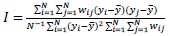 where N is the number of observational units; W = {wij}
12)Statistical tests point to no spurious relationship among the variables in the model. The unit root tests for our panel data suggest that all variables are non-stationary, and the panel cointegration tests indicate that the variables are cointegrated. This implies that national income, total capital, human capital, and infrastructure variables in levels (logged) are in a stable long-run relationship. Estimations results for non-spatial and spatial panel models with and without the estimated variable for non-infrastructure stock are presented in Appendix 3.
13)To address possible endogeneity between output and infrastructure capital stock, we also performed instrumental variables regression estimation for non-spatial and spatial models using the first lags of the infrastructure variable as instruments. The results are broadly similar to those from the ML estimation and are available upon request.
VI. Conclusions
This paper estimates direct benefits and cross-border spillover effects of transport (road and rail) & energy and ICT infrastructure (telephone, mobile, and broadband). Using the spatial panel regression models, we find a highly positive and significant impact of infrastructure, particularly transport & energy, on own countries. Furthermore, the positive externalities of rail, broadband, and human capital are found, and these results are robust in particular for broadband and human capital regardless of the choice of the spatial weight matrices.
Our finding on spillover effects of rail infrastructure provides support for the key role of other countries’ transport infrastructure on own country’s economies. The quality of infrastructure of trading partners is often highlighted as one of the major determinants that facilitate bilateral trade. For example, using the gravity model, Grigoriou (2007) finds that the infrastructure of neighboring countries is essential due to the transit effect in the landlocked Central Asian countries whose main modes of transportation to trade are road and rail.
It is worth highlighting that the cross-border spillover effect of broadband infrastructure is estimated to be larger than its within-country effect. This implies that increased access to the Internet can benefit not only own country’s economic growth, but also other neighboring economies to a higher extent. A positive link between higher Internet access and economic growth is also found in the literature (for example, Choi and Yi, 2009 and Pradhan et al., 2014).
Human capital also shows positive cross-border spillover effects on growth. Human capital activities involve not only transmission of available knowledge, but also the production of new knowledge which is the source of innovation and technical change (Mincer, 1981). Human capital positively affects productivity and thus educated labor has a much higher marginal product (Fleisher et al., 2008).
In sum, our empirical results confirm positive direct contributions of infrastructure, broadband infrastructure, and human capital on economic growth. More importantly, we find that their impacts are going even further beyond more than one country. This implies that transport network, access to Internet, and education show the nature of regional public goods since the benefits can be shared by public users across borders, contributing to regional growth. In particular the Internet, more broadly ICT has a large potential for Asia’s inclusive development, for example, by raising the equity, quality, and efficiency of education through ICT-enabled teaching and learning (ADB, 2017b).
Tables & Figures
Figure 1.
National Income vs Infrastructure by Type (2010-2014 average)

Note: Each dot represents a country in the sample; values are averages for 2010-2014.
Sources: Penn World Table 9.0
Figure 2.
Moran’s Scatter Plot for y

Note: W1 = {exp(-0.01*d)} is used; x axis is log(capita GDP); y axis is weighted average of neighboring countries log(per cap GDP)
Table 1.
Summary of Average Direct and Indirect Impacts on Output: Output Elasticity

TRE = transport and energy, ICT = information and communication technology
a For W2 (inverse distance weight matrix) only
b For W1 (exponential decay weight matrix) and W3 (square of inverse distance matrix with a cutoff) only
* = significant at the 90% or higher levels
Table 2.
Direct and Indirect Effects for Transportation & Energy (TRE)

Notes: Figures in parenthesis are robust standard errors; W1 = {exp(-0.01*d)}; W2 = {1/d}; W3 = {1/d2} with, all a 25th percentile cutoff; * p < 0.1, ** p < 0.05, and *** p < 0.01
Table 3.
Average Direct and Indirect Effects for ICT

Notes: Figures in parenthesis are robust standard errors; W1 = {exp(-0.01*d)}; W2 = {1/d}; W3 = {1/d2}, all with a 25th percentile cutoff; * p < 0.1, ** p < 0.05, and *** p < 0.01
Figure 3.
Long-term Spillover Effects of a 10% Increase in access to the Internet in PRC

Note: Countries shaded in gray are not available in the sample; the ICT model with the W3 is used to estimate the spillover effects; Boundaries are not necessarily authoritative.
APPENDIX 1. DATA DESCRIPTION
APPENDIX 2. CONSTRUCTION OF NON-INFRASTRUCTURE CAPITAL STOCK
Conceptually, the total capital stock  (in constant dollars;

where
•  = total infrastructure capital stock in constant dollars (unobserved);
  = total non-infrastructure capital stock in constant dollars (unobserved)
•  = infrastructure capital stock in quantity for type
  = the unit price of
  in the base year (unobserved)
•  = non-infrastructure capital stock in quantity for type
  = the unit price of
  in the base year (unobserved)
For simplicity, we assume that the unit prices reflect the depreciation of each capital stock item.
For each country, we regress the total capital stock on the infrastructure capital stock in quantity without a constant:

where the

where 
This leads us to express non-infrastructure capital as the residuals in Equation A11. For illustration purposes, we assume the Cobb-Douglas production function with infrastructure capital stock, non-infrastructure capital stock, and labor, and with constant returns to scale:

where  Equation (A11) is transformed into per-capita term and log-normalized for estimation:

where  are per capita infrastructure and non-infrastructure stock capital stock in constant dollars,
  is per capital infrastructure capital stock in quantity;
 is estimated as described in Equations A10-A11. Therefore,
  is the estimated coefficient of interest, output elasticity of infrastructure capital stock in quantity
  This is the approach that this study adopts.
On the other hand, in the case of when both total infrastructure stock and infrastructure stock in value are included, we show that the estimation results should be interpreted with caution as unknown values are part of the elasticity. We estimate:

where  is per capital total capital stock in constant dollars;
  It can be easily shown that the expected value of output elasticity of infrastructure capital stock in quantity becomes
  The term,
  represents country
APPENDIX 3. ESTIMATION RESULTS FOR NON-SPATIAL AND SPATIAL MODELS
Appendix Tables & Figures


Table A3.1
Estimation Results (Transportation & Energy: TRE) with Non-infrastructure Capital

Notes: 1) Original annual data with missing values for 1960-2014 are used; the other columns are when all variables are taken 5 year averages and missing values are imputed; 2) All variables are in logs; figures in parenthesis are robust standard errors; 3) W1 = {exp(-0.01*d)}; W2 = {1/d}; W3 = {1/d2}, all with a 25th percentile cutoff; 4) * p < 0.1, ** p < 0.05, and *** p < 0.01
Table A3.2
Estimation Results for ICT with Non-infrastructure Capital

Notes: 1) Original annual data with missing values for 1995-2014 are used; the other columns are when all variables are taken 5 year averages and missing values are imputed; For ICT-TC annual raw data, there are no broadband values for years 1995-1997; 2) All variables are in logs; figures in parenthesis are robust standard errors; 3) W1 = {exp(-0.01*d)}; W2 = {1/d}; W3 = {1/d2}, all with a 25th percentile cutoff; 4) * p < 0.1, ** p < 0.05, and *** p < 0.01
Table A3.3
Estimation Results (Transportation & Energy: TRE) with Total Capital

Notes: 1) Original annual data with missing values for 1960-2014 are used; the other columns are when all variables are taken 5 year averages and missing values are imputed; 2) All variables are in logs; figures in parenthesis are robust standard errors; 3) W1 = {exp(-0.01*d)}; W2 = {1/d}; W3 = {1/d2}, all with a 25th percentile cutoff; 4) * p < 0.1, ** p < 0.05, and *** p < 0.01
Table A3.4
Estimation Results for ICT with Total Capital

Notes: 1) Original annual data with missing values for 1995-2014 are used; the other columns are when all variables are taken 5 year averages and missing values are imputed; For ICT-TC annual raw data, there are no broadband values for years 1995-1997; 2) All variables are in logs; figures in parenthesis are robust standard errors; 3) W1 = {exp(-0.01*d)}; W2 = {1/d}; W3 = {1/d2}, all with a 25th percentile cutoff; 4) * p < 0.1, ** p < 0.05, and *** p < 0.01
References
-
Acemoglu, D. and J. A. Robinson. 2012.
Why Nations Fail: The Origins of Power, Prosperity and Poverty . New York, NY: Crown Publishers. -
Álvarez-Ayuso, I. C. and M. J. Delgado-Rodriguez. 2012. “High-capacity Road Networks and Spatial Spillovers in Spanish Regions,”
Journal of Transport Economics and Policy , vol. 46, no. 2, pp. 281-292. -
Asian Development Bank (ADB). 2017a.
Meeting Asia’s Infrastructure Needs . Abd.org eBook. <http://dx.doi.org/10.22617/FLS168388-2 > (accessed December 21, 2020) -
Asian Development Bank (ADB). 2017b.
Innovative Strategies for Accelerated Human Resource Development in South Asia: Information and Communication Technology for Education—Special Focus on Bangladesh, Nepal, and Sri Lanka . Abd.org eBook. <http://dx.doi.org/10.22617/TCS179 080 > (accessed December 21, 2020) -
Anselin, L. 2003. “Spatial Externalities, Spatial Multipliers, and Spatial Econometrics,”
International Regional Science Review , vol. 26, no. 2, pp. 156-166. -
Barro, R. J. and J. W. Lee. 2013. “A New Data Set of Educational Attainment in the World, 1950-2010,”
Journal of Development Economics , vol. 104, pp. 184-198.
-
Batey, P. W. and P. Friedrich. 2000.
Regional Competition . Berlin: Springer. - Berndt, E. R. and B. Hansson. 1991. Measuring the Contribution of Public Infrastructure Capital in Sweden. NBER Working Paper, no. 3842.
- Bhattacharyay, B. N. 2010. Estimating Demand for Infrastructure in Energy, Transport, Telecommunications, Water and Sanitation in Asia and the Pacific: 2010-2020. ADBI Working Paper Series, no. 248.
-
Boarnet, M. G. 1998. “Spillovers and the Locational Effects of Public Infrastructure,”
Journal of Regional Science , vol. 38, no. 3, pp. 381-400.
-
Calderón, C., Moral-Benito, E. and L. Servén. 2015. “Is Infrastructure Capital Productive? A Dynamic Heterogeneous Approach,”
Journal of Applied Econometrics , vol. 30, no. 2, pp. 177-198.
- Canning, D. and E. Bennathan. 1999. The Social Rate of Return on Infrastructure Investments. World Bank Policy Research Working Papers, no. 2390.
-
Choi, C. and M. H. Yi. 2009. “The Effect of the Internet on Economic Growth: Evidence from Cross-country Panel Data,”
Economics Letters , vol. 105, no. 1, pp. 39-41.
-
Cohen, J. and K. Monaco. 2007. “Ports and Highways Infrastructure: An Analysis of Intra- and Inter-state Spillovers,”
International Regional Science Review , vol. 31, no. 3, pp. 257-274.
- Égert, B., Kozluk, T. and D. Sutherland. 2009. Infrastructure and Growth: Empirical Evidence. OECD Economics Department Working Papers, no. 685.
-
Feenstra, R. C., Inklaar, R. and M. P. Timmer. 2015. “The Next Generation of the Penn World Table,”
American Economic Review , vol. 105, no. 10, pp. 3150-3182.
-
Fleisher, B. M., Li, H. and M. Q. Zhao. 2008. Human Capital, Economic Growth, and Regional Inequality in China. IZA Discussion Paper, no. 3576. <
https://www.econstor.eu/bitstream/10419/34981/1/573334765.pdf > (accessed December 21, 2020) -
Guild, R. L. 2000. “Infrastructure Investment and Interregional Development: Theory, Evidence, and Implications for Planning,”
Public Works Management & Policy , vol. 4, no. 4, pp. 274-285. <http://doi:10.1177/1087724X0044002 > (accessed October 21, 2020)
-
Grigoriou, C. 2007. Landlockedness, Infrastructure and Trade: New Estimates for Central Asian Countries. World Bank Policy Research Working Paper, no. 4335. <
https://openknowledge.worldbank.org/handle/10986/7294 > (accessed December 21, 2020) -
Hu, Z. and S. Luo. 2017. “Road Infrastructure, Spatial Spillover and County Economic Growth,”
IOP Conference Series: Materials Science and Engineering , vol. 231. <https://iopscience.iop.org/article/10.1088/1757-899X/231/1/012028 > (accessed December 22, 2020) -
International Road Federation (IRF). n.d. <
https://www.irf.global/statistics > (accessed October 21, 2020) -
International Telecommunication Union (ITU). n.d. <
https://www.itu.int/en/ITU-D/Statistics/Pages/default.aspx > (accessed October 21, 2020) -
LeSage, J. and R. K. Pace. 2009.
Introduction to Spatial Econometrics . Boca Raton: CRC Press. -
Lin, J., Yu, Z., Wei, Y. D. and M. Wang. 2017. “Internet Access, Spillover and Regional Development in China,”
Sustainability , vol. 9, no. 6. <https://doi.org/10.3390/su9060946 > (accessed December 22, 2020)
- Mincer, J. 1981. Human capital and economic growth. NBER Working Paper, no. 803.
-
Moshiri, S. 2016. “ICT Spillovers and Productivity in Canada: Provincial and Industry Analysis,”
Economics of Innovation and New Technology , vol. 25, no.8, pp. 801-820.
-
O’Mahony, M. and M. Vecchi. 2005. “Quantifying the Impact of ICT Capital on Output Growth: A Heterogeneous Dynamic Panel Approach,”
Economica , vol. 72, no. 288, pp. 615-633.
-
Organisation for Economic Co-operation and Development (OECD). 2002.
Measuring the Information Economy . OECD eBook. <https://www.oecd.org/sti/ieconomy/1835738.pdf > (accessed December 22, 2020) -
Pradhan, R. P., Arvin, M. B., Norman, N. R. and S. K. Bele. 2014. “Economic Growth and the Development of Telecommunications Infrastructure in the G-20 Countries: A Panel-VAR Approach,”
Telecommunications Policy , vol. 38, no. 7, pp. 634-649.
-
Sandler, T. 2006. “Regional Public Goods and International Organizations,”
The Review of International Organizations , vol. 1, no. 1, pp. 5-25.
-
Shahiduzzaman, M., Layton, A. and K. Alam. 2015. “On the Contribution of Information and Communication Technology to Productivity Growth in Australia,”
Economic Change and Restructuring , vol. 48, no.3-4, pp. 281-304.
-
Skorupinska, A. and J. Torrent-Sellens. 2015. “The Role of ICT in the Productivity of Central and Eastern European Countries: Cross-Country Comparison,”
Revista de Economía Mundial , vol. 39, pp. 201-222. <http://sem-wes.org/sites/default/files/revistas/07_TORRENT.pdf > (accessed December 22, 2020) -
Sloboda, B. W. and V. W. Yao. 2008. “Interstate Spillovers of Private Capital and Public Spending,”
The Annals of Regional Science , vol. 42, no. 3, pp. 505-518.
-
Tong, T., Yu, T.-H., Cho, S.-H., Jensen, K. and D. D. Ugarte. 2013. “Evaluating the Spatial Spillover Effects of Transportation Infrastructure on Agricultural Output across the United States,”
Journal of Transport Geography , vol. 30, pp. 47-55.
-
U.S. Energy Information Administration (EIA). n.d. <
https://www.eia.gov/tools > (accessed October 21, 2020) -
van Leeuwen, G. and H. van der Wiel. 2003. Spillover Effects of ICT. CPB Report, no. 2003/3. <
https://pdfs.semanticscholar.org/8e50/d4245c1b1d241d04f135e5ece2235ec51ab5.pdf > (accessed December 21, 2020) -
Wamboye, E., Adekola, A. and B. Sergi. 2016. “ICTs and Labour Productivity Growth in Sub-Saharan Africa,”
International Labour Review , vol. 155, no. 2, pp. 231-252.
-
Yu, N., de Jong, M., Storm, S. and J. Mi. 2013. “Spatial Spillover Effects of Transport Infrastructure: Evidence from Chinese Regions,”
Journal of Transport Geography , vol. 28, pp. 56-66.