
Bilingual dictionary generation and enrichment via graph exploration
Abstract
In recent years, we have witnessed a steady growth of linguistic information represented and exposed as linked data on the Web. Such linguistic linked data have stimulated the development and use of openly available linguistic knowledge graphs, as is the case with the Apertium RDF, a collection of interconnected bilingual dictionaries represented and accessible through Semantic Web standards. In this work, we explore techniques that exploit the graph nature of bilingual dictionaries to automatically infer new links (translations). We build upon a cycle density based method: partitioning the graph into biconnected components for a speed-up, and simplifying the pipeline through a careful structural analysis that reduces hyperparameter tuning requirements. We also analyse the shortcomings of traditional evaluation metrics used for translation inference and propose to complement them with new ones, both-word precision (BWP) and both-word recall (BWR), aimed at being more informative of algorithmic improvements. Over twenty-seven language pairs, our algorithm produces dictionaries about 70% the size of existing Apertium RDF dictionaries at a high BWP of 85% from scratch within a minute. Human evaluation shows that 78% of the additional translations generated for dictionary enrichment are correct as well. We further describe an interesting use-case: inferring synonyms within a single language, on which our initial human-based evaluation shows an average accuracy of 84%. We release our tool as free/open-source software which can not only be applied to RDF data and Apertium dictionaries, but is also easily usable for other formats and communities.
1.Introduction
Bilingual electronic dictionaries contain translations between collections of lexical entries in two different languages. They constitute very useful language resources, both for professionals (such as translators) and for language technologies (such as machine translation or the alignment of sentences in translated documents). Currently, we are witnessing an increase of such resources as linked data on the Web, owing to the adoption of linguistic linked data (LLD) techniques [6] by the language technologies community. That is the case of the Apertium RDF graph, built on the basis of the family of bilingual dictionaries of Apertium,11 a free-open/source machine translation platform [8]. A subset of 22 such dictionaries was initially converted into RDF (resource description framework),22 published as linked open data on the Web, and made available for access and querying in a way compliant with Semantic Web standards [13]. More recently, an updated version of the Apertium RDF graph has been released, covering 53 language pairs [11] (see Fig. 1).
Publishing bilingual dictionaries, and linguistic data in general, as linked data on the Web has a number of advantages. First, the data are described by using standard mechanisms of the Semantic Web, such as RDF and OWL (web ontology language33), and use consensual ontologies, agreed by the community, for their conceptual representation (such as Ontolex-lemon44 [28] in the case of the Apertium RDF). Further, it can be accessed through standard languages and query means such as the SPARQL protocol and RDF query language,55 avoiding any dependence on proprietary application programming interfaces (APIs). This enhances the availability, the interoperability, and the usability of the linguistic information that use such techniques [6]. In fact, every piece of lexical information (such as lexical entries, lexical senses, or translations) has its own URI, which identifies it at the Web scale and makes it easier to be linked to, or to be reused by, any other dataset or semantic-aware system developed for any purpose. For instance, the Apertium data, initially intended for their use in machine translation, has been successfully used, in its RDF version, for cross-lingual model transfer in the pharmaceutical domain [11]. In this application, an embeddings-based model for sentiment analysis in English was efficiently transferred into Spanish without retraining it from scratch, by injecting the English–Spanish translations contained in the Apertium RDF.
Fig. 1.
Graphical visualization of dictionaries in the Apertium RDF graph (figure taken from [11]), which covers 44 languages and 53 language pairs. The nodes represent monolingual lexicons and edges the translation sets among them. Darker nodes correspond to more interconnected languages.
![Graphical visualization of dictionaries in the Apertium RDF graph (figure taken from [11]), which covers 44 languages and 53 language pairs. The nodes represent monolingual lexicons and edges the translation sets among them. Darker nodes correspond to more interconnected languages.](https://content.iospress.com:443/media/sw/2022/13-6/sw-13-6-sw222899/sw-13-sw222899-g001.jpg)
In this work, we explore a method to automatically expand a graph of bilingual translations by inferring new translations based on the already existing ones. The method is agnostic of the particular graph formalism used to represent the data, although we apply it to the particular case of Apertium RDF. We further show how automatic dictionary generation is actually far more effective than reported in existing literature by developing evaluation methods that are better indicators of the actual utility. The motivation is two-fold: to support the evolution and enrichment of the Apertium RDF graph with new, automatically obtained high-quality data, and to support the Apertium developers when building new bilingual dictionaries from scratch as validating and adapting automatically predicted translations is easier for dictionary developers than writing new translation entries from scratch.
Fig. 2.
A small subgraph of translations based on the Apertium RDF. The shapes represent the semantic senses: black boxes, ‘bench’; red diamonds, ‘bench’ and ‘financial institution’; blue trapezium, ‘financial institution’ and ‘edge of a river’.
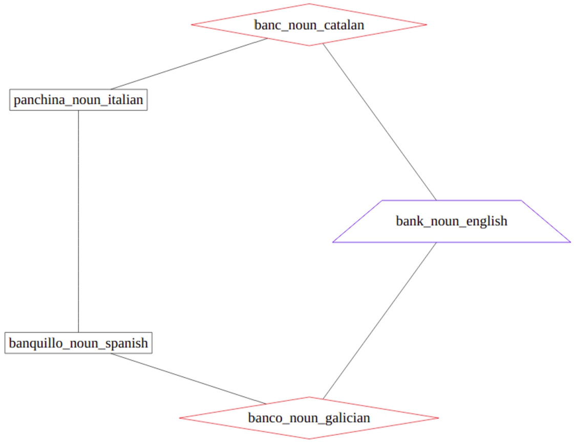
For instance, in Fig. 2, translations between nouns such as banc (Catalan) – banco (Galician), banco (Galician) – panchina (Italian), banc (Catalan) – banquillo (Spanish), are all valid but not present in the Apertium RDF. Our method tries to discover such indirect translations and assigns a confidence score to them. Our work is grounded on the approach proposed by Villegas et al. [34], based on the identification of dense cycles in the graph. We improve and extend this work in several directions:
– We improve the cycle-based algorithm by exploiting properties of biconnected graphs, which reduces execution time while discovering the same translations.
– We reduce the number of hyperparameters, and provide theoretical analysis for the ones chosen empirically in prior work, which reduces the search space for end users.
– We scale the experimental set-up to a much larger dataset, from two language pairs in the initial work (English–Spanish and English–French) up to 27 language pairs.
– We also measure the quality of predictions not found in the evaluation set through human evaluation and through validation with other available dictionaries, such as MUSE.66
We also contribute to the general translation inference problem in the following aspects:
– We demonstrate weaknesses of evaluation metrics used in existing literature that underestimate progress in translation inference. To this effect, we introduce and discuss novel metrics which are representative of performance and provide insights for further improvement.
– We propose a novel use case for the cycles-based method, the generation of synonyms.
As a result of this work, we release a modular and easily extensible software tool that can be used for practical dictionary generation (see Section 7). Currently, it supports RDF and the original Apertium format, but it can be easily extended to other communities and systems that need dictionary generation, simply by converting between their format and the internal tabulator-separated value (TSV) format.
The remainder of this paper is organized as follows: First, related work is summarized in Section 2. Then, Section 3 describes translation graphs, Section 4 describes the original cycle density algorithm [34], Section 5 describes the optimized version of the algorithm described in this work, Section 6 analyses the roles and need of each hyperparameter, Section 7 describes the software implementation, Section 8 describes the experimental settings of the study, novel evaluation metrics are proposed in Section 9, and the results are presented and discussed in Section 10. Use cases are discussed in Section 11 and, finally, Section 12 presents some conclusions and future work.
2.Related work
The automatic generation of electronic bilingual dictionaries based on existing ones is not a new research topic. Several approaches have been proposed over the last few decades. In this section we give an overview of the main ones.
2.1.Pivot-based methods
The simplest approach is to assume that the translation relation is transitive. This method assumes the existence of two bilingual dictionaries, one containing translations from language
However, the translation relation is not always transitive, as polysemy in the pivot language could lead to wrong translations being inferred. For instance in Fig. 2, the Catalan (
In order to overcome this issue and identify incorrect translations when constructing bilingual dictionaries mediated by a third language, Tanaka and Umemura [32] proposed in 1994 a method called one-time inverse consultation (OTIC). In short, the idea of the OTIC method is, for each word w in
OTIC was later adapted for different purposes, such as the creation of multilingual lexicons from bilingual lists of words [22]. While OTIC is intended for generic dictionaries, similar methods have been developed for generation of domain-adapted bilingual dictionaries [18]. Other authors have enriched OTIC with the inclusion of semantic features, such as Bond and Ogura [5] for the creation of a Japanese–Malay dictionary. Saralegi et al. [31] studied how to use distributional semantics computed from comparable corpora to prune pivot-based translations.
2.2.Graph-based methods
The works referred so far illustrate techniques that take into account the existence of (at least) two language pairs connected through a common pivot. However, when dictionaries can be connected in a richer way as part of a larger graph, other algorithms based on graph exploration may come into play. That is the case, for instance, of the CQC algorithm, developed by Flati and Navigli [7], which exploits the notion of cycles and quasi-cycles (hence the acronym CQC) for the automated disambiguation of translations in a bilingual dictionary. Notice that, unlike our approach, this method is not intended for dictionary building but for dictionary validation. Another remarkable method based on graph exploration is the SenseUniformPaths algorithm proposed by Mausam et al. [25], which relies on probabilistic methods to infer lexical translations. SenseUniformPaths was used in the generation of PanDictionary [26], a massive translation graph built from 630 machine-readable dictionaries and Wiktionaries,88 which contain over 10 million words in different languages and 60 million translation pairs. The method applies probabilistic sense matching to infer lexical translations between two languages that do not share a translation dictionary. To that end, they define circuits (cycles with no repeated vertices), calculate scores for the different translation paths, and prune those circuits that contain nodes that exhibit undesirable behaviour, called correlated polysemy (see Section 4.1).
The SenseUniformPaths algorithm served as the basis for the cycle density method proposed by Villegas et al. [34] that we explore and expand in this work. SenseUniformPaths also uses cycles to identify potential translation targets, but the method by Villegas et al. differs in that it uses the graph density of cycles to rate the confidence value. This cycle density algorithm does not need to identify ambiguous cycles, and is therefore computationally less expensive. Moreover, SenseUniformPaths exploits dictionary senses, as found in resources such as Wiktionary while the cycle density method can operate in dictionaries without such sense information, such as the Apertium bilingual dictionaries, and therefore solves a harder problem.
2.3.Distributional semantics-based methods
Other methods have also been proposed that do not rely on graph exploration for bilingual lexicon induction, but are based on distributional semantics. Initial approaches have been based on vector space models [30,35] or in leveraging statistical similarities between two languages [9,16]. More recent approaches that exploit distributional semantics rely on the inference and use of cross-lingual word embeddings. An initial contribution in that direction was made by Mikolov et al. [29]. Methods using word embeddings to infer new dictionary entries require an initial seed dictionary that is used to learn a linear transformation that maps the monolingual embeddings into a shared cross-lingual space. Then, the resulting cross-lingual embeddings are used to induce the translations of words that are missing in the seed dictionary [3].
Such ideas evolved and new embeddings-based methods appeared that did not need such initial training, such as the work by Lample et al. [21], who propose a method to develop a bilingual dictionary between two languages without the need of using parallel corpora. The method needs large monolingual corpora for the source and target languages and leverages adversarial training to learn a linear mapping between the source and target spaces. The software implementing the method and the ground-truth bilingual dictionaries used to test it are publicly available.99 We use these ground-truth dictionaries as part of our evaluation (Section 9.3).
Another remarkable method of this embeddings-based family of techniques was developed by Artetxe et al. [4]. In their work, instead of directly inducing a bilingual lexicon from cross-lingual embeddings as in [21], they use the embeddings to build a phrase table, combine it with a language model, and use the resulting machine translation system to generate a synthetic parallel corpus, from which the bilingual lexicon is extracted using statistical word-alignment techniques.
In contrast to graph-based methods, the embeddings-based approaches still need large corpora to operate, which limits, for example, their applicability for under-resourced languages. Moreover, they operate at the word representation level, and therefore do not take into account other lexical information such as the part of speech, which can be essential to disambiguate the semantic sense of the word.
2.4.Systematic evaluation
The fact that inferring new translations is not a trivial problem has motivated the Translation Inference Across Dictionaries (TIAD)1010 periodic shared task, as a coherent experimental framework to enable reliable comparison between methods and techniques for automatically generating new bilingual (and multilingual) dictionaries from existing ones. A number of works, based on graph exploration, word embeddings, parallel corpora, etc. have participated so far in the campaign to test their ideas, many of them preliminary and subject to continuous improvement [12,19,27].
2.5.Comparison with OTIC
As the TIAD campaign has showed, the OTIC algorithm continues to be a powerful method for translation inference, and it has proven to be very effective even in comparison with more contemporary methods [12,19]. However, OTIC needs a pivot language to operate, while cycle-based systems can discover translations between more indirectly connected languages. For instance, out of 946 possible language pairs in Fig. 1, pivot-based methods are applicable to 145 pairs which have a pivot, whereas the cycle density method that we study in this article can be applied to any of the 414 connected pairs. As an example, OTIC cannot work for Sardinian (sc) – Galician (gl) whereas the cycle-based method is able to infer translations between them. On the other hand, there can be less connected parts of the graph where dense cycles are difficult to find, where OTIC performs better. For instance, English (en) – Russian (ru) in the Apertium RDF.
Cycle-based methods can be used for additional tasks, such as synonym generation (see Section 11.2), which OTIC is not able to address. Moreover, cycle-based procedures are more suitable for iterative dictionary enrichment, as the produced translations for a target language pair (
In parallel work, a recent contribution to TIAD [10] demonstrates that OTIC and the cycle density algorithm can be combined into a generalized Augmented Cycle Density (ACD) framework that leverages their complementary advantages. Built on top of our released open-source tool and insights, ACD is a state-of-the-art procedure, outperforming both the OTIC and cycle density algorithm individually. In particular, in the TIAD 2021 official evaluations,1111 ACD achieved an average
3.Translation graph
We define translation graph as an undirected graph
Note that G is initially populated using multiple bilingual dictionaries at once. Since the input translations (and hence the graph edges) are between words of different languages (
In particular, we have used the latest version (v2.1) of the Apertium RDF graph as our initial translation graph.1212 It contains 44 languages and 53 language pairs, with a total number of translations
Our problem is now to enrich this initial graph G, that is, to infer edges that do not initially exist but define valid translations.
4.The original cycle density method
In this section, we describe with more detail the cycle density method developed by Villegas et al. [34], which we base this work on.
4.1.Cycles in the translation graph
As mentioned in Section 2, the original algorithm relies on simple cycles instead of transitive chains, following the idea of circuits introduced in [25]. A simple cycle is a sequence of vertices starting and ending in the same vertex with no repetitions of vertices and edges. For ease of explanation, we will be referring to simple cycles as just cycles.
For a sequence of words
4.2.Confidence metric: Cycle density
There can be multiple instances of correlated polysemy in a single cycle. In fact, considering that many language pairs in Apertium are linguistically close, this is not unexpected. Therefore, approaches based on exploiting sparsely inter-connected partitions of cycles may not be fruitful, as our experience has shown. Accordingly, we stick to using cycle density as proposed in [34] as a metric to avoid invalid predictions due to correlated polysemy.
The density of a subgraph
A higher density implies that the nodes in a cycle are closer to forming a clique. Therefore, intuitively, for high-density cycles, completing the clique by predicting the pairs of words with no edge between them as possible translations becomes a useful strategy, one which we adopt. In cases with correlated polysemy, subsets of vertices corresponding to a different set of senses are unlikely to have any edges between them, leading to a lower cycle density. In Fig. 2, there are 5 edges out of a possible 10, giving a density of 0.5. Thus, a density threshold higher than 0.5 will prevent (
4.3.Original algorithm
The algorithm outlined in [34] is summarized in the following lines. For each word w do the following:
1. Find the D-context of w, which is the subgraph
2. Find all cycles in
3. The confidence score of a translation from w to u not directly connected in the input data to w is the density of the densest cycle containing both w and u.
4. Impose further constraints on possible translations to improve empirical results such as (see Section 6.2 for more detail):
(a) not allowing language repetition within a cycle, that is, one word per language only;
(b) ignoring cycles with size under a particular minimum length
(c) requiring a lower confidence score for target nodes u that have a higher degree than 2 in the subgraph induced by the cycle.
5.Improving the efficiency of the cycle density method
In order to allow for application scenarios in which time performance is an important feature as well as to facilitate scalability to larger graphs, our first modifications to the cycle density method were aimed at making computation more efficient, without having any negative impact on the quality of the inferred translations.
Notice that the algorithm requires us to operate on cycles, and cycle-finding is essentially a bottleneck in terms of computation time, even after having established a bound on the maximum cycle length. Optimizing cycle-finding is essential for scaling to larger graphs, and also allows end users to make multiple runs with different hyperparameter settings, which can be important for achieving optimal results on the languages or language pairs 1313 that are of interest to them.
The original implementation of the cycle density method1414 computes and stores all cycles up to length
5.1.Precomputing biconnected components
A biconnected graph is one in which no vertex exists such that removing it disconnects the graph. A biconnected component is a maximal biconnected subgraph.1515
Different biconnected components can only share cut vertices, that is, vertices whose removal renders the graph disconnected. The decomposition of a graph
Property 1.
Consider any two vertices u, v in the same biconnected component. There must be at least one simple cycle with vertices only in the biconnected component containing both u and v.
Proof.
There must be at least two vertex-disjoint (apart from u and v) paths from u to v. Combining these 2 vertex-disjoint paths would give a simple cycle, as the graph is undirected. Otherwise, if all paths from u to v within the component have a common vertex w, removing w would disconnect u and v and this is not possible in a biconnected component by definition. □
Property 2.
For every simple cycle C, there exists a biconnected component B such that
Proof.
A simple cycle is in itself a biconnected graph. It must therefore be a subgraph of some biconnected component. □
Property 2 tells us that we can run the algorithm separately for each biconnected component without missing any cycle, and consequently any translation. Property 1 shows us that biconnected components are in some sense the minimal units such that decomposing them further would make us lose information. Finding all cycles takes a number of operation which is exponential on the number of edges; therefore, by splitting a graph into smaller subgraphs, we require much less computation. Mathematically, this follows from
The empirical speed-up is demonstrated in Table 1. Note that the improvement on lexicon-wide experiments like in Table 1 is partially shadowed by the cycle finding algorithm we use (see Section 5.3), which already implicitly exploits the locality of the graph. The partition into biconnected components is more useful when searching for translations of specific words instead of the entire vocabulary in one go. A lookup table file mapping words to biconnected components can be maintained. This helps load only the biconnected components the word belongs to instead of the entire graph, which cuts both computation time and memory requirements.
Table 1
For our lexicon-wide experiments, splitting into biconnected components reduces time by about a third on average compared to when we are not. The development and large data sets contains 11 and 27 language pairs respectively (see details in Section 8)
| Data set | Computed on | Time range (sec) |
| Development | biconnected | 10–15 |
| entire graph | 17–23 | |
| Large | biconnected | 22–57 |
| entire graph | 33–80 |
5.2.Filtering cross-part-of-speech translations
Although it is not frequent, there might be cases in RDF dictionaries in which translations connect words with different POS. As shown in Table 2, by removing such cases, large biconnected components containing multiple POS can be further split into smaller ones with just one POS. Our method takes that step in order to reduce run-time, and to prevent potentially spurious inferred translations.
Table 2
Size of the entire graph (G) and largest biconnected component (
| Case | ||||
| All translations | 704,284 | 774,986 | 84,088 | 188,116 |
| No cross-POS | 704,284 | 769,708 | 44,542 | 99,081 |
In Table 3 we present the distribution of number of biconnected components by size on our large set of 27 language pairs (see Section 8) after discarding the cross-POS translations.
Table 3
Distribution of biconnected component size in the main graph containing 27 language pairs
| Size | 4–5 | 6–10 | 11–20 | 21–100 | >100 |
| # | 7,193 | 5,520 | 1,847 | 262 | 7 |
While clearly most biconnected components are small, some are indeed quite large, which is evident from the size of the largest one as shown in Table 2.
There are situations, however, where users might need to keep such cross-POS translations. For instance, in Apertium one can find a translation of the English noun computer into the Spanish adjective informático. This allows for rules, in a machine translation system, that may translate noun modifiers such as computer engineer as adjectives to get fluent translations such as ingeniero informático by looking up these cross-POS entries in the dictionary. This is especially important when the target languages do not have the same set of POS, requiring changes in POS during translation. Therefore, any implementation of the method should make this filter optional.
5.3.Backtracking search per source word
Within each biconnected component, we iterate over all words as the source word and repeat the following procedure for finding possible target words: First, we find and store the context graph of depth D for word w,
6.Analysis of hyperparameters
The heuristic indicators used in the original cycle density method were derived empirically by studying small parts of the RDF graph. Scaling to larger vocabulary-wide experiments requires generalizing these heuristics to tunable hyperparameters. To that end, a deeper understanding of such hyperparameters is needed. Ideally, language pair developers should be able to iteratively run the algorithm, verify and include the correct translations, and then repeat the process on the updated, richer graph, getting new entries each time. This necessitates reducing the eight distinct indicators proposed originally [34] and limiting the combinations that need to be tried to obtain optimal results. Through our exploratory analysis of the hyperparameters we describe in this section, we reduce both runtime and human effort.
6.1.Removed hyperparameters
After a careful analysis, we found that a number of heuristics and hyperparameters proposed in [34] were not leading to better results, therefore we propose to discard them:
Language repetition: The intuition for removing cycles with language repetition as in [34] is that two words in the same language are likely to not have the exact same set of semantic senses. Example: pupil in English can mean the aperture of the iris, but will also come in cycles with student. This can become a breeding ground for correlated polysemy, leading to incorrect translations. But allowing language repetition is necessary to generate synonyms (see Section 11.2); this would necessitate making this optional by adding a binary hyperparameter.
Furthermore, we find that not allowing repetition reduces recall significantly, and the same higher precision can instead be achieved by increasing the confidence threshold for a lesser loss in recall. Handling correlated polysemy is exactly what measuring cycle density is aimed at, so it is a natural way to mitigate this issue. We therefore proceed to remove this hyperparameter.
Minimum cycle length: Notice that cycle density as defined in Section 4.2 would favour shorter cycles, as the denominator grows quadratically with cycle length. In particular, a 4-cycle without any other edges among its vertices would have a density of
This is why the original algorithm [34] requires a minimum cycle length. In fact, they require different minimum lengths for a large context and a small context because in relatively sparse areas of the graph, many cycles might be small and yet correct. This leads to having three hyperparameters that require tuning: the minimum length in small contexts, the minimum length in large contexts, and the threshold defining when a context becomes large.
However, we found that eliminating all three hyperparameters gives similar results on average, while simplifying the pipeline significantly. Allowing small cycles allows more translations to be produced, as ignoring them completely would also leave out the probably valid translations we could predict using the dense small cycles.
6.2.Used hyperparameters
Having eliminated four hyperparameters of the original cycle density method, we now justify why we need the remaining ones and find the most suitable range of values for them.
Maximum cycle length (
1. With increasing distance1616 from the source vertex, the chances of sense shifting increase. Thus, larger cycles have a higher chance of being polysemous.
2. Induced graphs of large cycles will probably have as subgraphs smaller cycles with higher density. These smaller cycles get selected as the ones with the highest density for most pairs of words. This means allowing larger cycles does not lead to the generation of many new translations.
Context depth (D): Similarly to the cycle length, the original motivation for limiting context depth was to reduce computation time. We find that increasing it beyond a certain threshold is not helpful because of the following property:
Property 3.
It is lossless to keep
Proof.
If cycle length is limited to
This effectively sets an upper bound to the context depth based on the maximum cycle length. We recommend using
Target degree multiplier (M): Here, by the degree of a vertex, we refer to the number of edges from the vertex within the subgraph induced by the cycle. Originally, in [34], a fixed lower (0.5 instead of 0.7) confidence threshold (density) was required for cycles if the target word had degree
Transitivity (T): While an essential premise to necessitate a cycle-based approach is that transitivity does not always hold for translations due to polysemy, we realized that it can still perform well for non-polysemous categories of words.1717 Specifically, we identify proper nouns and numerals as being largely non-polysemous. Both categories are part of the LexInfo ontology,1818 a catalogue of grammar categories used by the Apertium RDF. We model transitivity as a ternary hyperparameter:
Confidence threshold (C): For a given pair of words u, v, let
Note that we stick to only the cycle with the highest confidence. We prefer this over metrics that use aggregate statistics over all the cycles containing the two words, such as the number of cycles or their average density. These are more likely to be sensitive to some subgraphs or contexts being richer in the number of translations added during creation, leading to superfluously better aggregates than others. The maximum is more robust to these differences, as only one dense cycle is then sufficient.
For translations produced using transitivity (
This motivates the final choice the user makes, the confidence threshold C. Generated translations above this confidence threshold are all included in the final prediction set of the algorithm.
To conclude, we have a set of just four simple hyperparameters: context depth D, maximum cycle length
We have shown that a fixed value for context depth relative to the maximum cycle length is optimal in most cases. Moreover, the procedure is not very sensitive to the target degree multiplier within a reasonable range of
7.Implementation
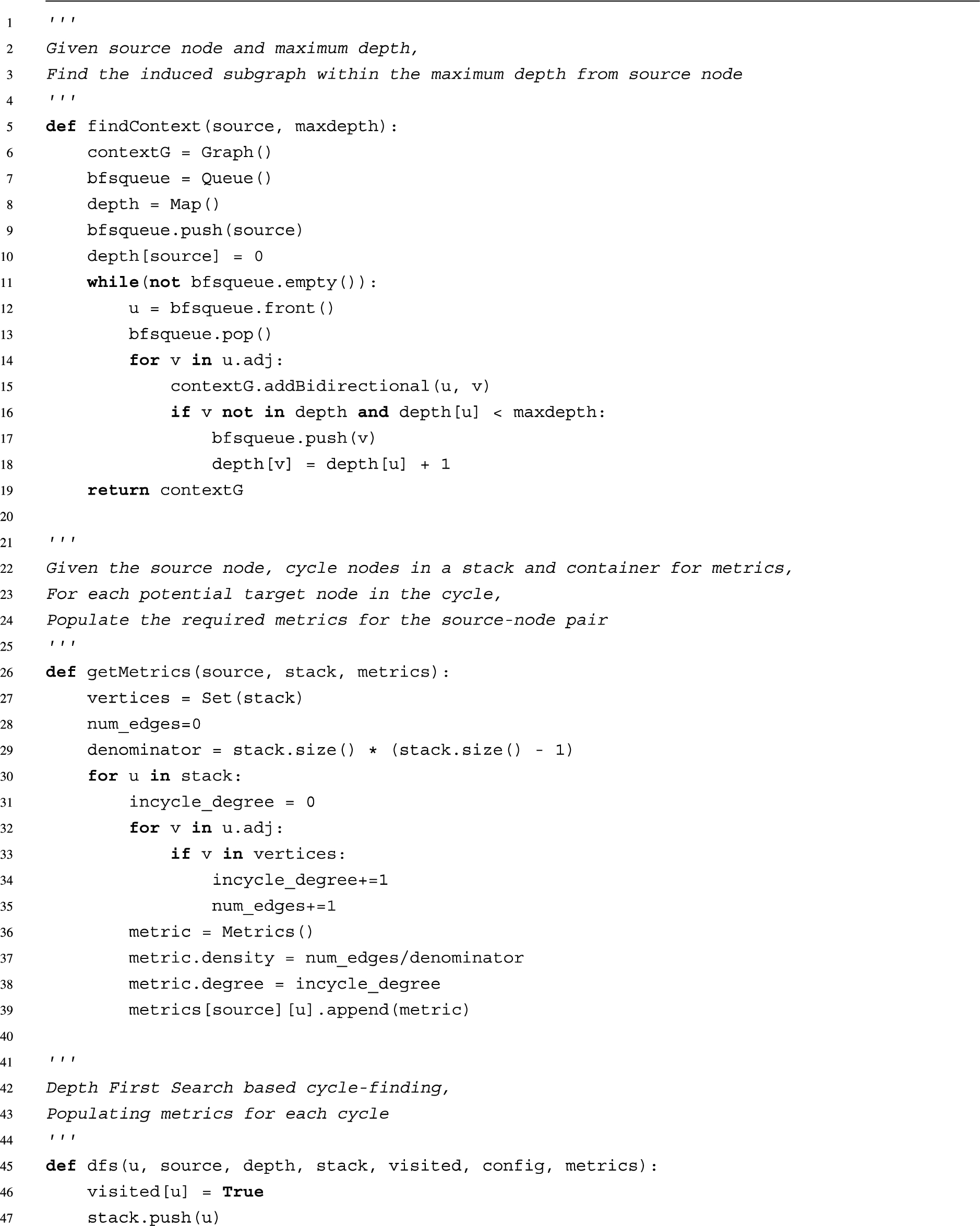
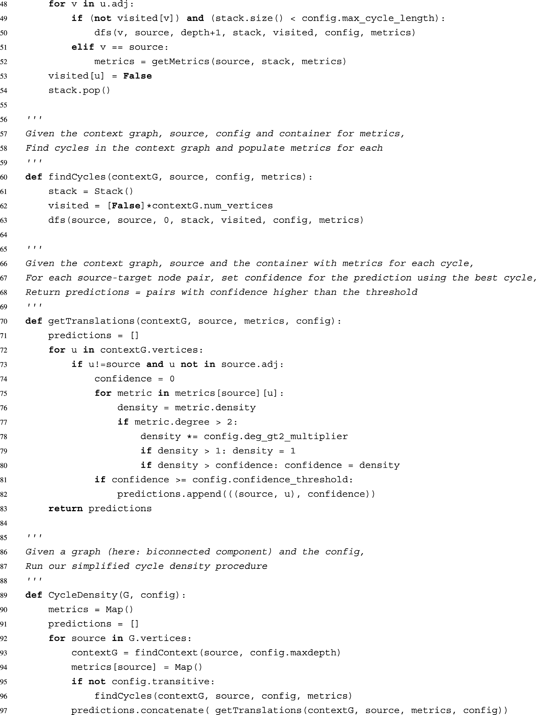
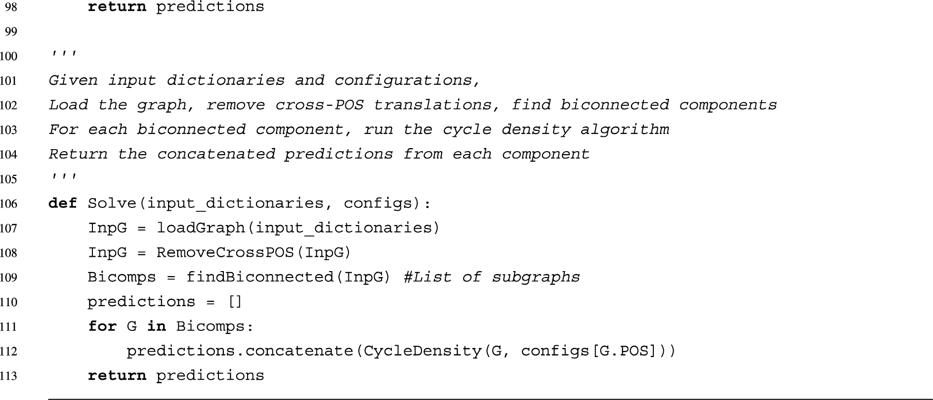
We implemented the algorithmic pipeline in C++. Detailed instructions for usage are provided in our GitHub repository.2121 The pseudocode for our final algorithm is provided in Appendix x. It has been simplified to convey the core logic, for example, we omit describing the trivial transitive selection of translations which is a useful option for some POS.
Using the command line options provided in our tool, translations can be generated for specific language pairs, across all language pairs or for a single word. If the same language is specified in the pair, such as eng-eng, synonyms are generated. Different configurations of the hyperparameters can be provided for each POS.
A simple format has been defined to represent the data of an input translation graph
8.Experimental setting
There are two main possible usage scenarios for the cycle density method: (i) generation of a new bilingual dictionary from scratch for a new language pair, and (ii) enrichment of an already existing language pair. In order to measure the effectiveness of the method in the first case, we remove one already existing language pair (dictionary) from the graph, try to re-create it with the algorithm, and then compare the result with the removed dictionary. In the second case, entirely new translations are created, which are more difficult to evaluate automatically. Nevertheless, to provide a quality indication, we propose the use of external bilingual dictionaries that are not part of the Apertium graph as well as a human evaluation.
8.1.Datasets
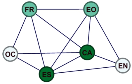
For initial experimentation with metrics and hyperparameter tuning, we picked a development set of 11 language pairs across 6 languages: English, Catalan, Spanish, Esperanto, French, and Occitan (see Fig. 3). We leave out each language pair and use the remaining 10 to re-generate it. This allows us to measure average metrics across the 11 language pairs.
Fig. 3.
Fragment of the Apertium RDF graph taken as development set, containing 6 languages and 11 language pairs.
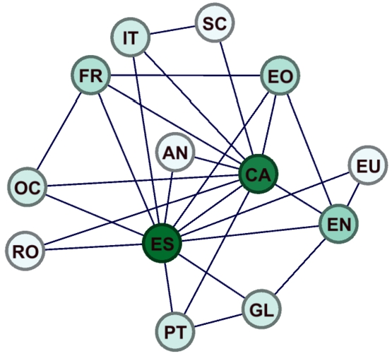
Since one of our goals in this research is to scale up the initial cycle density algorithm, it is important to validate that the method performs well even when more language pairs come into play. To that end, we define what we call the large evaluation set, by taking all 27 language pairs across the 13 languages which constitute the largest biconnected component in the RDF language graph (see Fig. 4).2222 These languages are: Aragonese, Basque, Catalan, English, Esperanto, French, Galician, Italian, Occitan, Portuguese, Romanian, Sardinian and Spanish.
We use the same leaving-one-pair-out experiment as the development set in this new setting, reporting average metrics across the 27 language pairs.
Fig. 4.
Languages in the largest biconnected component in the Apertium RDF graph. It contains 13 languages and 27 language pairs.
In general, if a user wants to predict translations for a target language pair
8.2.Hyperparameter settings
After experimenting with the development set, the final hyperparameter setting, used across the rest of the evaluation, is the following (unless otherwise specified): transitive closure (
8.3.Baseline
As mentioned earlier, one of the main usage scenarios of the cycle density algorithm is the generation of new bilingual dictionaries for the Apertium framework. The idea is to substitute the cross option provided as part of the apertium-dixtools in Apertium (see Section 2) which relies on transitive inference [33]. Therefore, we introduce in our experiments an explicit comparison with a method that is purely based on transitivity, which we emulate by running our system with two sets of hyperparameters:
8.4.External dictionaries
In order to validate the enrichment of translations in already existent language pairs, we use the MUSE ground truth dictionaries2323 as an additional corpus. MUSE dictionaries, while rich in nouns, verbs, adjectives, adverbs and numerals, have almost no proper nouns. We thus stick to translations in these five POS categories for our experiments. There are five MUSE dictionaries that are common to our large set: English–Catalan, English–Spanish, French–Spanish, Spanish–Italian, Spanish–Portuguese, which we use for our experiments.
9.Evaluation
When evaluating procedures aimed at generation, a fundamental problem arises when an exhaustive ground-truth set is not available. Having an exhaustive set of translations turns out to be particularly hard because languages keep evolving. Today’s complete set will become incomplete soon, as the vocabulary of the languages grow. Moreover, many languages are low-resourced, and obtaining sets with high coverage itself is a difficult task.
While the in-production Apertium language pairs are large enough to be useful for a machine translation engine, their coverage can clearly be increased. In the forthcoming discussion, we assume that while available evaluation sets may reasonably be considered to have 100% precision (ground truth),2424 they do not carry all possible valid translations. Moreover, it is even difficult to estimate the total number of valid translations.
9.1.Notation
We begin by defining some notation we will use throughout the following sections.
– I denotes the input translation graph, which could include multiple bilingual dictionaries.
– P denotes the translation graph containing the predictions (output) of the algorithm. In our experiments, we generate a single language pair, and hence P can be considered the graph of the predicted target language pair.
–
– T denotes the translation graph of the chosen test dictionary for evaluation. This is the left-out RDF dictionary for pair
– A denotes the hypothetical complete set of valid translations for language
–
–
–
9.2.Metrics for automatic evaluation
The unavailability of a complete test dictionary makes it difficult to measure traditional metrics like precision (
9.2.1.Both-Word Precision (BWP)
It is clear that the precision computed using any T is a lower-bound on the actual precision of the algorithm, as
A predicted translation
1.
2.
3.
4.
Therefore, we propose measuring precision only among those predicted translations for which both words are in the test dictionary. We define this as both-word precision
Note that if the test dictionary has both words but no edge between them, this could still be due to oversight by the creators. The computed BWP is again a lower-bound for the actual BWP. Using a larger test dictionary
9.2.2.Both-Word Recall (BWR)
Achieving a high precision often entails that the prediction set produced has less coverage and hence low recall. However, this could be due to insufficient input data or misalignment between the distributions of the input set and the test dictionary. It can thus be useful to normalize by how much of the test dictionary can possibly be generated using a given input set by a hypothetically perfect algorithm. Specifically, if for
It can thus be useful to limit our evaluation set to those translations for which both words are in the input set. Therefore, we define both-word recall (BWR) as
Moreover, in our experiments, I consists of other RDF dictionaries. These dictionaries are likely to contain the frequently used words, and evaluation set translations which do not have the corresponding words in the input graphs are probably among less frequent, specific words. Thus, BWR can in some tasks be a measure of how much of the important part of the left-out language pair we cover.
We would like to note that the BWR metric, while good at evaluating different modifications to the same algorithmic pipeline (such as different hyperparameter settings), should be used carefully when comparing two methods that use different input datasets. This is because
9.3.Measuring dictionary enrichment with external data
While external corpora can be used for evaluating additional translations, they often have significantly different properties from the input and target sets. This can lead to erroneous conclusions due to noisy results.
However, evaluating against additional data is particularly important in the context of this paper for the following reasons:
– It is a direct accuracy indicator on the task of enrichment.
– It can also verify how tight the lower bounds that BWP provides are, as well as whether BWP is a good substitute for precision.
– For the case of recall, while computing it against completely new data is generally not a good idea, we can verify that the BWR metric is much more robust to dataset distribution differences than vanilla recall by computing both on this new test set.
We use the MUSE dictionaries (see Section 8.4) to evaluate the quality of additional translations.
9.4.Measuring dictionary enrichment with human assessment
As a final sanity check of our additional entries, we took random samples of 150 predicted dictionary entries that were not present in the test set T. These belonged to open POS categories, that is, nouns, adjectives, adverbs, verbs and proper nouns, and also numerals. This was done directly using Apertium bilingual dictionaries as input data with a rather liberal (recall-oriented) set of hyperparameters:
As these sets were produced with a different version of the data and hyperparameters, we took an intersection between these sets and the additional translations produced by a different setting that need to be evaluated. While this is not directly a random sample of the additional translations, it is a good approximation.
10.Results and discussion
In this section we show and discuss the experimental results of our evaluation. For the sake of brevity, we show here an aggregated view of the results, but we make all the experimental data available online to allow further inspection.2727
In the following discussion, we define relative size as
Furthermore, we use the BWP and vanilla recall metric for computing F-scores. We prefer BWP over precision as it is far more indicative, and the vanilla precision metric is noisy as shown in Table 5. We have to choose vanilla recall over BWR, as recall uses the same target set (
We begin by showing our optimal results on the development set in Table 10 (first row). Each metric is averaged across the 11 language pairs. The computation time differs for each language pair to be generated, so we report the range (minimum–maximum).
Notice the significant gap between BWR and recall, showing the scope for improvement in the algorithm’s results if the input RDF graph is enriched. Since our procedure itself can iteratively aid such enrichment, we hope that in the future this gap will be bridged. Moreover, the BWP is much larger than the precision, which shows that evaluation schemes based on precision could be grossly underestimating the performance of algorithms on this task, when the actual insufficiency is in the test data.
We also report statistics in Table 4 for the 9 most frequent POS. The other POS have a too small number of translations to give reliable results.
Table 4
Relative size for different parts of speech, averaged across the language pairs in the development set
| POS | Noun | Verb | Proper noun | Adjective | Adverb | Determiner | Numeral | Pronoun | Preposition |
| Rel. Sz. | 55.04% | 57.03% | 497.99% | 43.44% | 43.22% | 45.65% | 211.28% | 59.25% | 74.27% |
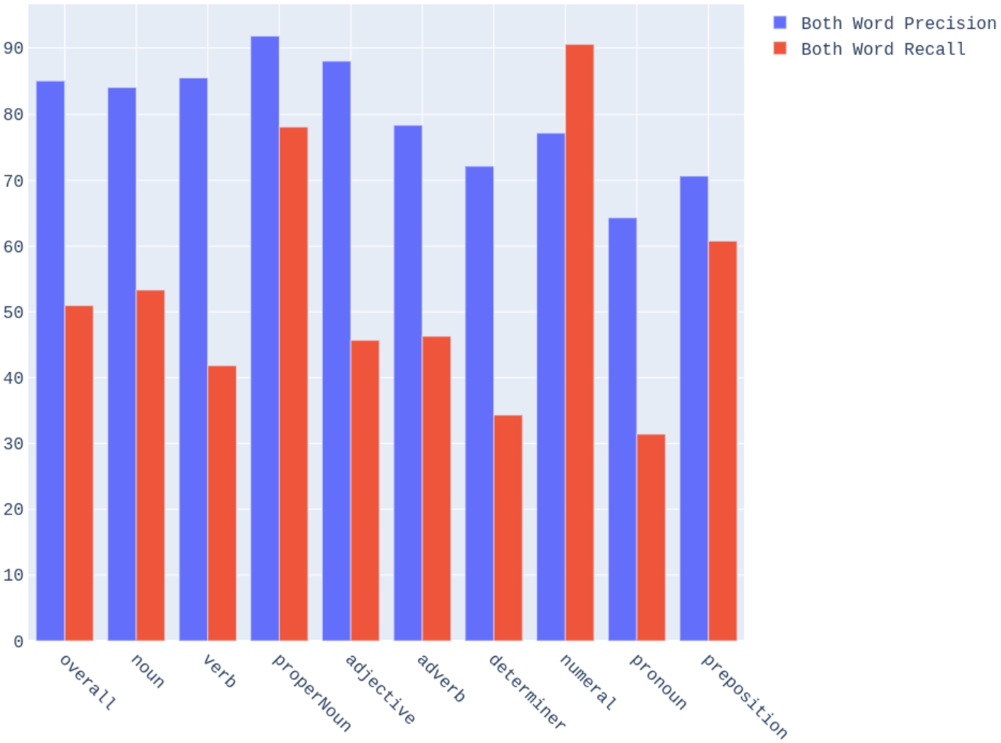
Table 4 shows that the transitive closure adopted produces much more translations of proper nouns and numerals than the existing Apertium dictionaries. Yet, the BWP in Fig. 5 is quite high for proper nouns, and decent for numerals. Moreover, our procedure has high precision for open POS, and less for closed POS. This is because the translations of closed POS in Apertium often encode grammatical changes which are context specific and not semantic equivalencies. Thus, when such closed POS translations are leveraged to produce new ones in our system, the results are less likely to be correct than open POS. It might still be helpful to use more restrictive hyperparameters or a higher confidence threshold when producing translations of closed POS.
Fig. 5.
Breakdown by POS of BWP (left bars) and BWR (right bars), averaged across language pairs in the development set.
10.1.Demonstrating hyperparameter changes
Table 5 shows how decreasing the confidence threshold C while holding all hyperparameters constant leads to lower BWP and higher BWR, recall and prediction set size as expected. The end user can tune this precision-recall tradeoff to their liking (see Section 11.1 for a discussion in the context of Apertium), but we stick to maximizing the
Table 5
Change in results when varying the confidence threshold
| C | BWP | Prec. | BWR | Recall | |
| 0.4 | 81.60% | 46.36% | 52.11% | 29.96% | 50.86% |
| 0.5 | 85.00% | 48.37% | 50.96% | 29.32% | 50.93% |
| 0.6 | 86.39% | 48.93% | 48.68% | 27.94% | 50.25% |
| 0.7 | 87.80% | 48.55% | 42.24% | 24.19% | 47.35% |
| 0.8 | 89.52% | 48.40% | 37.98% | 21.69% | 45.24% |
Table 6 shows that increasing the maximum allowed cycle length keeping all else constant leads to decreasing BWP, but increasing BWR, recall and time. We see diminishing returns in the
Table 6
Change in results when varying the maximum cycle length
| BWP | BWR | Recall | Time (s) | ||
| 4 | 89.53% | 30.50% | 15.94% | 30.24% | 7–9 |
| 5 | 86.69% | 49.39% | 28.33% | 50.43% | 8–10 |
| 6 | 85.00% | 50.96% | 29.32% | 50.93% | 10–15 |
| 7 | 81.96% | 51.56% | 29.66% | 50.31% | 15–22 |
| 8 | 76.67% | 52.35% | 30.12% | 47.92% | 30–50 |
Next, Table 7 shows the comparison for proper nouns and numerals between using the hyperparameter setting used for other POS and the chosen
Table 7
Benefit from using transitivity for proper nouns and numerals
| POS | T | BWP | BWR | Recall |
| Proper nouns | 0 | 98.47% | 24.75% | 11.95% |
| 2 | 91.81% | 78.11% | 32.81% | |
| Numerals | 0 | 97.66% | 55.64% | 35.22% |
| 2 | 77.17% | 90.55% | 61.27% |
To demonstrate the extent of polysemy in the RDF Graph, we use the
Table 8
Average metrics across 11 language pairs in the dev. Set when using
| BWP | BWR | Recall | Rel. Sz. | |
| 15.26% | 81.11% | 46.81% | 718.75% | 23.94% |
Finally, we show in Table 9 that allowing language repetition actually improves performance, which led us to removing the hyperparameter.
Table 9
Average metrics across 11 language pairs when not allowing language repetition compared to when it is allowed
| Repetition | BWP | BWR | Recall | Rel. Sz. | |
| Allowed | 85.00% | 50.96% | 29.32% | 75.73% | 50.93% |
| Restricted | 86.89% | 46.81% | 28.49% | 73.03% | 49.45% |
10.2.Dictionary generation
In Table 10 we present the results of transferring the same hyperparameter setting derived in our development set to our large set, continuing the dictionary generation experiment but with a larger graph. It takes longer to run, but still within one minute for all language pairs. Once again, the accuracy metrics reported are averaged across the 27 language pairs that are left-out one by one.
The drop in the metrics on the large set compared to the development set is not necessarily a sign of overfitting. The large set has more less-connected, under-resourced language pairs, which bring down the averages.
Table 10
Results of the cycle density algorithm on average metrics in the development and large sets
| BWP | BWR | Recall | Rel. Sz. | Time range (sec) | ||
| dev set | 85.00% | 50.96% | 29.32% | 75.73% | 50.93% | 10–15 |
| large set | 84.07% | 40.98% | 25.95% | 71.39% | 35.90% | 22–57 |
In Table 11, we demonstrate a significant gain in relative size across POS when using the large set compared to Table 4 when using the development set. Similar trends are observed for BWR in Fig. 7. In Fig. 6 we show the variation in the metrics across the 27 languages in the large set. While a high BWP is maintained across all language pairs, the prediction set size varies greatly based on the richness of Apertium RDF entries in the input. Some of the language pairs with the lowest number of translations produced are: por–glg (6,044), spa–por (10,176), eus–spa (12,243). On the other hand, language pairs with the highest number of translations produced are: spa–cat (50,145), eng–cat (52,323), fra-cat (68,087). This is consistent with Catalan (cat) having some of the largest dictionaries in the Apertium RDF, whereas Portuguese (por) and Basque (eus) ones are much smaller.
We show a comparison between the cycle density algorithm and the transitive baselines in Table 12. We see that transitive closure tends to increase relative coverage and recall, but at the cost of a much lower precision (55% and 13% for the respective baselines vs. 84% for cycle density). Depending on the use case, a balance towards recall might be acceptable, but usually a decent level of precision is important, which the transitive procedures do not provide. As expected, baseline 2 produces many more candidate translations, leading to a much larger prediction set but dropping precision significantly.
In order to measure the impact of enriching the input graph towards improving results, in Table 13 we also restrict the averaged metrics to the 11 development set language pairs, still using the whole large set as input. There is a significant improvement in comparison with the original development set experiments (see Table 10). This demonstrates the advantages of adding more input data. Notice how in this scenario, due to the fact that language pairs are more connected, the cycle density algorithm beats the transitive baselines in terms of the F1-score as well.
Table 11
Relative size for different POS, averaged across the 27 language pairs in the large set
| POS | Noun | Verb | Proper noun | Adjective | Adverb | Determiner | Numeral | Pronoun | Preposition |
| Rel. size | 70.78% | 81.75% | 539.29% | 59.39% | 61.99% | 53.48% | 241.53% | 80.32% | 107.10% |
Fig. 6.
Boxplot showing, left to right: BWP, recall,
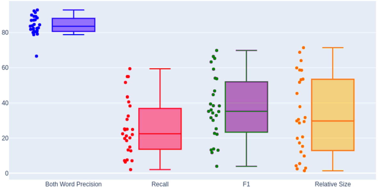
Fig. 7.
Breakdown by POS of BWP (left bars) and BWR (right bars), averaged across language pairs in the large set.
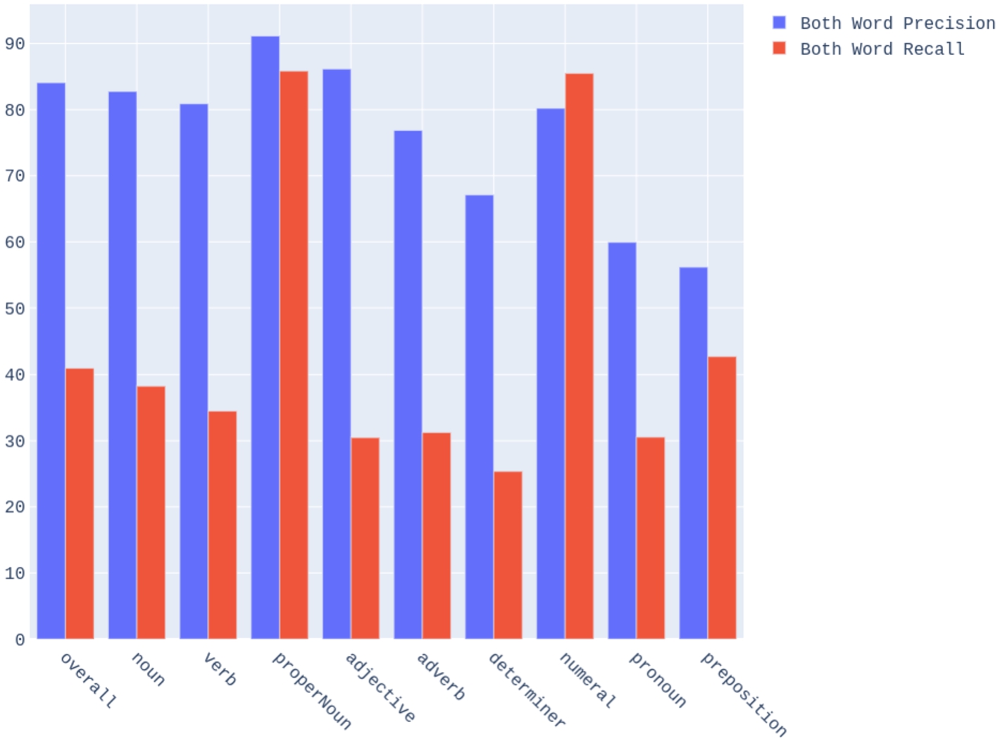
Table 12
Comparing the baselines 1 and 2 (
| BWP | BWR | Recall | Rel. size | ||
| Cycle density | 84% | 41% | 26% | 71% | 36% |
| Baseline 1 | 55% | 85% | 56% | 237% | 42% |
| Baseline 2 | 13% | 88% | 57% | 1038% | 19% |
Table 13
Comparing the baselines 1 and 2 (
| BWP | BWR | Recall | Rel. size | ||
| Cycle density | 81% | 56% | 36% | 94% | 51% |
| Baseline 1 | 48% | 81% | 53% | 267% | 44% |
| Baseline 2 | 11% | 83% | 54% | 1176% | 17% |
In conclusion, our produced translations are on average 71.39% the size of existing Apertium dictionaries at a high BWP of 84.07% across 27 language pairs over 13 languages.
10.3.Dictionary enrichment
Fig. 8.
Breakdown of the match between the predicted set P, the original test s, and the input set I. For all word classes (overall) and for words in each lexical category, each left bar is divided from bottom to top, to show overall precision (predicted word correspondences in P which are in the original apertium dictionary used as test set T), and then the percentages of additional predicted word correspondences with both words in the test set (both with original), with the left word in the test set (left with original), with the right word in the test set (right with original), and with neither word in the test set (neither with original). Also for all word classes (overall) and for words in each lexical category, each right bar is divided also from bottom to top, to show overall recall (word correspondences in the test set T which are in the predicted set P), and then the percentages of missed word correspondences in the test set T with both words in the input set I (both with input), with the left word in the input set (left in input), with the right word in the input set (right in input), and with neither word in the input set (neither in input). Refer to the discussion in Sections 10.3 and 9.2.
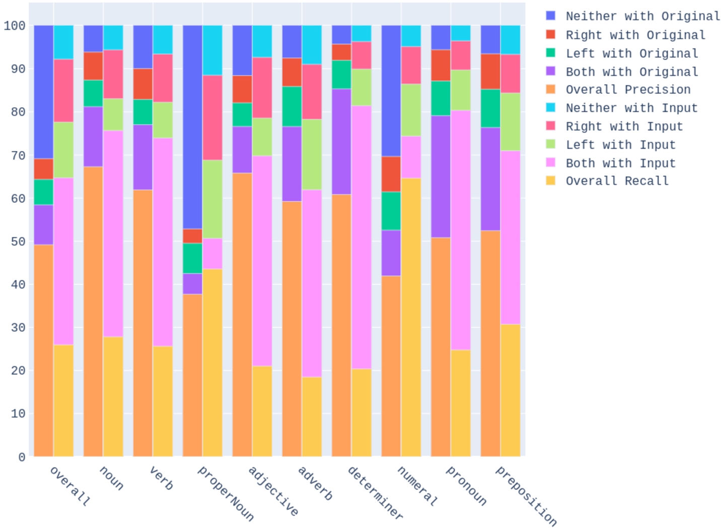
The coloured bar graph in Fig. 8 shows statistics about the predicted translations in P that match the test set T and contrasts it with those that do not match, which are further classified. These are average metrics reported over the 27 language pairs in the large set.
In particular, it classifies the additional translations in P (the left bar) in terms of how many words they have in common with the original Apertium dictionary used as a test set, T, and classifies the missed translations (the right bar) of T in terms of how many words they have in common with the input set I. This also provides a way to visualize the BWP and BWR metrics defined in Sections 9.2.1 and 9.2.2 respectively. From bottom to top, the BWP (resp. BWR) is the ratio of the height of the lowest sub-bar to the combined height of the lowest two sub-bars in the left (resp. right) bars.
As has been said, Fig. 8 shows the ratios of different additional (resp. missed) translations based on the words shared with the target original Apertium dictionaries used as test set T (resp. input Apertium dictionaries I) in the left (resp. right) bar of each POS. Almost 30% of predicted translations have neither word in the test set. This is particularly high due to the large relative size in proper nouns and numerals and demonstrates the incompleteness of original Apertium dictionaries, which implies there is a vast scope for enrichment. On the other hand, while the number of missed translations with neither word in the input data is just 10%, for over 30% of test set translations only one word is present in the input data. This demonstrates the scope for improving the algorithm’s recall by improving the coverage of the input data for specific languages. A similar analysis can be done on a more fine-grained level for each POS.
We now evaluate the additional translations for the 5 language pairs also present in MUSE (see Section 8.4). In Table 14, we calculate the overall BWP of our additional translation set with MUSE as test set. We further show the breakdown of the additional translations in terms of number of words shared with our original test set, that is, the left-out RDF dictionary. Particularly,
Table 14
BWP for different classes of additional translations based on words shared with original test set evaluated using MUSE
| Lang. pair | BWP | ||||||
| eng–cat | 15.57% | 156 | 80.00% | 978 | 41.99% | 2268 | 6.90% |
| eng–spa | 35.64% | 315 | 94.02% | 575 | 51.89% | 374 | 17.78% |
| fra–spa | 65.97% | 2218 | 94.94% | 239 | 39.83% | 105 | 11.08% |
| spa–ita | 37.88% | 108 | 76.05% | 53 | 32.31% | 47 | 19.34% |
| spa–por | 54.72% | 353 | 78.97% | 131 | 38.98% | 31 | 19.62% |
Table 15 shows a comparison between BWR and recall with MUSE as the test set (T) using the algorithm’s output prediction sets (P) when given the large set as input (I). While the recall is dismal, the BWR is much higher, in fact somewhat similar to the BWR on the actual test sets in the large experiments, when we evaluate on the left-out dictionary instead of MUSE. This shows that the BWR is relatively insensitive to the dataset distributions and thus a robust metric for evaluation.
Table 15
Recall vs. BWR when comparing predictions using the large set with MUSE dictionaries
| Lang. pair | Recall | BWR |
| eng–spa | 7.05% | 53.24% |
| eng–cat | 8.84% | 49.81% |
| epo–eng | 8.76% | 59.69% |
| fra–cat | 0.97% | 7.94% |
| oci–fra | 2.63% | 23.51% |
Finally, we report accuracy for the additional translations predicted during the large experiment on the human evaluation sets in Table 16. The precision obtained is encouraging, confirming that our procedure works well for enrichment. Note that the varying sample size is due to the dataset difference and intersection taken explained in Section 9.4.2929
Table 16
Accuracy of additional translations based on human evaluation
| Lang. pair | Sample size | Precision |
| eng–spa | 133 | 78.94% |
| eng–cat | 67 | 77.61% |
| epo–eng | 146 | 80.13% |
| fra–cat | 130 | 69.23% |
| oci–fra | 134 | 84.32% |
10.4.Recommending the use of BWP and BWR
BWR should be used as a valuable test metric when the same input dataset is used, particularly by creators when tuning and improving a particular algorithm. It also signifies the data-effectiveness of any proposed algorithm. It gives a clear picture of the optimization landscape, growing more consistently than recall as the prediction set becomes more liberal, as shown in Table 8.
BWP can be used for comparison across systems to make evaluation of translation inference pipelines more accurate. A natural usage scenario for this metric is the TIAD shared task. In particular, the evaluation procedure in TIAD (until the 2020 edition) modified traditional precision metrics in the same direction as in this paper by limiting the output set for precision to translations for which the word in the source language is in the evaluation set. This is somewhat what we could call one-word-precision, but the key drawback is that it is asymmetric. The precision computed for language pair
11.Use cases
In this section we give more details on the application of the cycle density algorithm to support generation and enrichment of dictionaries in the Apertium framework, and introduce another use case, which is the discovery of synonym words in the same language.
11.1.Apertium
As mentioned above, Apertium3030 [8] is a free/open-source rule-based machine translation system; that is, the information it needs to translate from one language to another is provided in the form of dictionaries and rule sets. Bilingual dictionaries are, therefore, a key component of the data used for a language pair. Apertium language data is all released using the GNU General Public Licence,3131 a free/open-source licence. This has, in particular, made it easy for derivatives of Apertium bilingual dictionaries to be published such as lexical-markup framework (LMF) dictionaries,3232 and the RDF dictionaries mentioned in this paper [11,13]. Methods like ours can be used to extend or create Apertium bilingual dictionaries.
It has to be noted though that the LMF and RDF dictionaries do not contain all the information present in the Apertium bilingual dictionaries, but just the orthographic representation (spelling) of the lemma and the POS; Apertium dictionaries may contain additional information, for instance, to inform of the fact that the gender of a word changes (so that, for instance, target-side gender agreement with adjectives is ensured by an appropriate rule), as in this Spanish–Catalan entry,
<e a="gema">
 <p>
   <l>almohada<s n="n"/><s n="f"/></l>
   <r>coixí<s n="n"/><s n="m"/></r>
 </p>
</e>
where in addition of the fact that the Spanish (left, l) lemma almohada(‘pillow’) is a noun (n) corresponding to the Catalan (right, r) lemma coixíwith the same part of speech, the entry also encodes the fact that almohadais a feminine (f) noun and coixíis a masculine (m) noun. In entries where the gender does not change, this is usually not indicated. Therefore, some of the bilingual correspondences predicted by our tool in its current form may need to be completed after being validated by an Apertium expert. Work is in progress to add this information to the RDF graphs and to improve the method described here to be able to transfer morphological information to predicted entries directly.
When Apertium experts process each predicted dictionary entry, they first validate its usefulness and then either discard it or adopt it, perhaps adapting it by inserting additional information (like gender), before adding it to the dictionary. The actual time required to do these operations may be used to inform the weight β that should be given to recall in an
11.2.Discovering synonyms
We have until now discussed the usage of our algorithm for creating bilingual dictionaries. The same cycle density procedure however can also be used to generate edge predictions between words in the same language, that is, synonyms. This allows extending from generating just dictionaries to even creating thesauri.
In fact, some popular translation engines like Google Translate also provide synonyms to end users, unlike Apertium. Automatic synonym generation from Apertium data could thus help create a useful feature. Synonymy relations may also be useful represented as linguistic linked data.
The confidence score obtained in our method can also possibly be used as a measure for conceptual similarity. Traditional methods based on word co-occurrence suffer from several issues for this task, requiring further augmentation [24]. In-fact, it has even been shown that having translation information is one way to improve their performance [14]. Our method takes that hypothesis to the extreme, relying purely on translation graphs over documents. Some advantages of this are as follows:
– Our method does not need large corpora, which can be hard to obtain for under-resourced languages. Besides, it does not require complex augmentation procedures and is interpretable as the subgraph that leads to each prediction can be identified.
– Since antonyms often occur in similar contexts in sentences, they are assigned high similarity by co-occurrence based methods. Our method does not appreciably suffer from such problems.
– Co-occurrence based methods ignore polysemy. They are known [23] to perform suboptimally when finding synonyms for polysemous words because they aggregate statistics across the different semantic senses [2]. On the other hand, our approach is explicitly polysemy-aware.
We demonstrate here a preliminary experiment. We produce synonym pairs for English, Spanish and Catalan using the large set of 27 language pairs as input. Random samples of 150 words drawn from the 3 prediction sets are evaluated by 2 human annotators each, and we report the results in Table 17. To the evaluators, we pose a similar question as before: “Is there a context where the two words are replaceable?”.
Table 17
Human evaluation of predicted synonym pairs. κ denotes the Cohen Kappa as a measure of inter-annotator agreement between the 2 annotators for each language
| Language | Prediction set (# pairs) | Precision | κ |
| English | 9,652 | 76% | 0.4291 |
| Spanish | 7,664 | 88.66% | 0.5574 |
| Catalan | 10,254 | 87.33% | 0.1581 |
Note that we took the same hyperparameters and confidence threshold as the translation setting (see 8.2). Modifications specific to synonym generation might be required for optimal results. The results demonstrated are just a proof of concept, more detailed studies and exact comparisons with existing methods are left for future work.
12.Conclusions and future work
This paper has explored techniques that exploit the graph nature of openly available bilingual dictionaries to infer new bilingual entries. We leverage the knowledge that independent Apertium developers have separately encoded in different language pairs. The techniques build upon the cycle density method of [34], which has been modified (taking advantage of graph-theoretical features of the dictionary graphs) so that it is faster and has less hyperparameters to adjust when applying it to a task. We release our tool as a free/open-source software which can be applied to RDF graphs but also directly to Apertium dictionaries.
We further show that existing automatic evaluation metrics for dictionary inference have limitations. To this end, we propose two metrics for automatic evaluation of the dictionary inference task, both-word precision and both-word recall, and show extensively how they help to compare and improve existing dictionary algorithms. The notion of such metrics could have been used implicitly in earlier work, but we provide a formal definition, as well as an extensive analysis and comparison with traditional metrics.
We experiment with a large portion of the Apertium RDF graph on two bilingual dictionary development scenarios: dictionary creation for a new language pair, and dictionary enrichment. The results show how the progressive enrichment of the translation graph leads to better results with the cycle density method, and confirm its superiority with respect to transitive-based baselines. Moreover, our evaluations based on external dictionaries (MUSE) and human assessment show that a significant amount of additional translations, not initially found in the graph, are correct. We also illustrate that the algorithm can be used to infer synonyms, unlike pivot-based methods, and report a human-based evaluation on this.
We highlight the following opportunities for future work:
– Enrich the cloud of linguistic linked data by applying the method to other datasets, and connect the Apertium RDF with other families of dictionaries on the Web.
– Exploit the fine-grained morphological information, beyond POS, that is sometimes present in Apertium bilingual entries.
– Improve the performance of the synonym generation through more elaborate evaluation and include it as a feature in Apertium.
– Explore the ability of k-connectedness (for
– Use topological methods like the ones highlighted here to study polysemy from the perspective of linguistic typology and connect it with studies in cognitive science that use translation graphs to study semantic mapping across languages [37].
– Study the feasibility of an iterative approach in which validated predictions are fed back in each round to produce additional predictions.
– Explore more optimal methods that directly find the maximum density cycles under additional constraints posed by our hyperparameters without having to compute all cycles within a certain length, perhaps with inspiration from maximum density subgraph methods [20].
– Study how language pair developers use our tool to understand their preferences in the precision–recall trade-off, using these insights to improve evaluation metrics.
– Participate in upcoming editions of the TIAD task for more direct comparisons with other systems.
– Explore the complementary use of cycle based techniques with pivot-based ones like OTIC.
Notes
12 The Apertium RDF data dumps, developed by Goethe University Frankfurt, are available in Zenodo through this URL: https://tinyurl.com/apertiumrdfv2. More details on the generation of Apertium RDF v2 can be found at [11]. A stable version of Apertium RDF v2 will be uploaded to http://linguistic.linkeddata.es/apertium/ and hosted by Universidad Politécnica de Madrid (UPM) as part of the Prêt-à-LLOD H2020 project.
13 Generating dictionaries for particular language pairs is a popular instance of the more general dictionary enrichment problem.
15 More generally, a k-connected graph is one which remains connected if fewer than k vertices are removed.
16 Defined here as the length of the shortest path between two vertices.
17 This is partly why we allow different hyperparameter settings for different POS.
19 Not used in this paper, it exists for ongoing exploration towards future work.
20 We still keep it as a hyperparameter as it can make the confidence score more reflective of the similarity, which might be important for some use-cases.
22 Notice that, although loosely related to the notion of training, development and test sets in machine learning, the purpose of creating our development and large sets is slightly different, being targeted towards confirming scalability. The hyperparameters will ultimately be manually tuned by the users to adapt the system to their particular needs.
24 Apertium dictionaries (and hence the derived RDF dictionaries) do have some translations that may not be considered “correct”, so they are not 100% precise as assumed, but such errors are limited in number and do not affect evaluation significantly.
25 See Fig. 8 and the corresponding discussion for a visual understanding of this metric, and the above categories.
26 We had 3 evaluators for the first 3 language pairs, so we consolidated their differences using a simple majority vote to produce the gold standard. For the last two we had a single evaluator whose results became the gold standard.
28 This can be larger than 100% if the prediction set is larger than the evaluation set.
29 The small sample for eng–cat is potentially due to some substantial difference in the Apertium bilingual dictionaries and the Apertium RDF version we use, analysing which is beyond the scope of this paper.
31 Versions 2 (https://www.gnu.org/licenses/old-licenses/gpl-2.0-standalone.html) and 3 (https://www.gnu.org/licenses/gpl-3.0-standalone.html).
32 Such as the LMF Apertium dictionaries in https://repositori.upf.edu/handle/10230/13034 and https://github.com/apertium-lmf.
33 Note that validating and adopting may be done faster than validating and rejecting, as to do the latter operation safely one would need to think harder about possible contexts.
Acknowledgements
We thank Google for its support through Google Summer of Code 2020. S. Goel thanks the Apertium community and Kunwar Shaanjeet Grover for helpful discussions. We also thank Gema Ramírez, Hèctor Alós i Font, Aure Séguier, Silvia Olmos, Mayank Goel and Xavi Ivars for their evaluation of predicted dictionary entries. This work was partially funded by the Prêt-à-LLOD project within the European Union’s Horizon 2020 research and innovation programme under grant agreement no. 825182. This article is also based upon work from COST Action CA18209 NexusLinguarum, “European network for Web-centred linguistic data science”, supported by COST (European Cooperation in Science and Technology). It has been also partially supported by the Spanish projects TIN2016-78011-C4-3-R and PID2020-113903RB-I00 (AEI/FEDER, UE), by DGA/FEDER, and by the Agencia Estatal de Investigación of the Spanish Ministry of Economy and Competitiveness and the European Social Fund through the “Ramón y Cajal” program (RYC2019-028112-I).
Appendices
Appendix
AppendixPseudocode of the algorithm
References
[1] | R.E.L. Aldred and C. Thomassen, On the maximum number of cycles in a planar graph, Journal of Graph Theory 57: (3) ((2008) ), 255–264. doi:10.1002/jgt.20290. |
[2] | S. Arora, Y. Li, Y. Liang, T. Ma and A. Risteski, Linear algebraic structure of word senses, with applications to polysemy, Transactions of the Association for Computational Linguistics 6: ((2018) ), 483–495. doi:10.1162/tacl_a_00034. |
[3] | M. Artetxe, G. Labaka and E. Agirre, Learning principled bilingual mappings of word embeddings while preserving monolingual invariance, in: Proceedings of the 2016 Conference on Empirical Methods in Natural Language Processing, (2016) , pp. 2289–2294. doi:10.18653/v1/D16-1250. |
[4] | M. Artetxe, G. Labaka and E. Agirre, Bilingual lexicon induction through unsupervised machine translation, in: Proc. of 57th Annual Meeting of the Association for Computational Linguistics (ACL 2019), Association for Computational Linguistics (ACL), (2019) , pp. 5002–5007. ISBN 9781950737482. doi:10.18653/v1/p19-1494. |
[5] | F. Bond and K. Ogura, Combining linguistic resources to create a machine-tractable Japanese-Malay dictionary, Language Resources and Evaluation 42: (2) ((2008) ), 127–136. doi:10.1007/s10579-007-9038-4. |
[6] | P. Cimiano, C. Chiarcos, J.P. McCrae and J. Gracia, Linguistic Linked Data, Springer International Publishing, (2020) . ISBN 978-3-030-30224-5. doi:10.1007/978-3-030-30225-2. |
[7] | T. Flati and R. Navigli, The CQC algorithm: Cycling in graphs to semantically enrich and enhance a bilingual dictionary, Journal of Artificial Intelligence Research 43: ((2012) ), 135–171. doi:10.1613/jair.3456. |
[8] | M.L. Forcada, M. Ginestí-Rosell, J. Nordfalk, J. O’Regan, S. Ortiz-Rojas, J.A. Pérez-Ortiz, F. Sánchez-Martínez, G. Ramírez-Sánchez and F.M. Tyers, Apertium: A free/open-source platform for rule-based machine translation, Machine translation 25: (2) ((2011) ), 127–144. doi:10.1007/s10590-011-9090-0. |
[9] | P. Fung and L. Yuen Yee, An IR approach for translating new words from nonparallel, comparable texts, in: Proc. of 17th International Conference on Computational Linguistics (COLING 1998), ACL, (1998) , pp. 414–420, https://www.aclweb.org/anthology/C98-1066. |
[10] | S. Goel and K.S.S. Grover, From pivots to graphs: Augmented CycleDensity as a generalization to one time inverse consultation, in: Proc. of 4th Translation Inference Across Dictionaries (TIAD 2021) @ LDK’21, (2021) , [in press]. |
[11] | J. Gracia, C. Fäth, M. Hartung, M. Ionov, J. Bosque-Gil, S. Veríssimo, C. Chiarcos and M. Orlikowski, Leveraging linguistic linked data for cross-lingual model transfer in the pharmaceutical domain, in: Proc. of 19th International Semantic Web Conference (ISWC 2020), B. Fu and A. Polleres, eds, Springer, (2020) , pp. 499–514. ISBN 978-3-030-62465-1. doi:10.1007/978-3-030-62466-8-31. |
[12] | J. Gracia, B. Kabashi, I. Kernerman, M. Lanau-Coronas and D. Lonke, Results of the translation inference across dictionaries 2019 shared task, in: Proc. of TIAD-2019 Shared Task – Translation Inference Across Dictionaries Co-Located with the 2nd Language, Data and Knowledge Conference (LDK 2019), J. Gracia, B. Kabashi and I. Kernerman, eds, CEUR Press, Leipzig (Germany), (2019) , pp. 1–12. doi:10.5281/ZENODO.3555155. |
[13] | J. Gracia, M. Villegas, A. Gomez-Perez and N. Bel, The apertium bilingual dictionaries on the web of data, Semantic Web 9: (2) ((2018) ), 231–240. doi:10.3233/SW-170258. |
[14] | F. Hill, K. Cho, S. Jean, C. Devin and Y. Bengio, Not All Neural Embeddings are Born Equal, 2014. doi:10.48550/arXiv.1410.0718. |
[15] | J. Hopcroft and R. Tarjan, Algorithm 447: Efficient algorithms for graph manipulation, Commun. ACM 16: (6) ((1973) ), 372–378. doi:10.1145/362248.362272. |
[16] | A. Irvine and C. Callison-Burch, Supervised bilingual lexicon induction with multiple monolingual signals, in: Proc. of NAACL-HLT 2013, Association for Computational Linguistics, (2013) , pp. 9–14, https://www.aclweb.org/anthology/C98-1066/. |
[17] | D.B. Johnson, Finding all the elementary circuits of a directed graph, SIAM J. Comput. 4: (1) ((1975) ), 77–84. doi:10.1137/0204007. |
[18] | H. Kaji, S. Tamamura and D. Erdenebat, Automatic construction of a Japanese-Chinese dictionary via English, in: Proc. of the Sixth International Conference on Language Resources and Evaluation (LREC’08), European Language Resources Association (ELRA), (2008) . |
[19] | I. Kernerman, S. Krek, J.P. Mccrae, J. Gracia, S. Ahmadi and B. Kabashi, Introduction to the globalex 2020 workshop on linked lexicography, in: Proc of Globalex’20 workshop on linked lexicography at LREC 2020, in: ELRA, I. Kernerman, S. Krek, J.P. McCrae, J. Gracia, S. Ahmadi and B. Kabashi, eds, (2020) . ISBN 979-10-95546-46-7. |
[20] | S. Khuller and B. Saha, On finding dense subgraphs, in: ICALP’09, Springer-Verlag, Berlin, Heidelberg, (2009) , pp. 597–608. ISBN 9783642029264. doi:10.1007/978-3-642-02927-1_50. |
[21] | G. Lample, A. Conneau, A. Ranzato, L. Denoyer and H. Jégou, Word translation without paralell data, in: Proc. of 6th International Conference on Learning Representations (ICRL 2018), (2018) . |
[22] | L.T. Lim, B. Ranaivo-Malançon and E.K. Tang, Low cost construction of a multilingual lexicon from bilingual lists, Polibits 43: ((2011) ), 45–51. doi:10.17562/pb-43-6. |
[23] | F. Liu, H. Lu and G. Neubig, Handling homographs in neural machine translation, in: Proceedings of the 2018 Conference of the North American Chapter of the Association for Computational Linguistics: Human Language Technologies, Volume 1 (Long Papers), Association for Computational Linguistics, New Orleans, Louisiana, (2018) , pp. 1336–1345. doi:10.18653/v1/N18-1121. |
[24] | A. Lu, W. Wang, M. Bansal, K. Gimpel and K. Livescu, Deep multilingual correlation for improved word embeddings, in: Proceedings of the 2015 Conference of the North American Chapter of the Association for Computational Linguistics: Human Language Technologies, Association for Computational Linguistics, Denver, Colorado, (2015) , pp. 250–256. doi:10.3115/v1/N15-1028. |
[25] | Mausam, S. Soderland, O. Etzioni, D. Weld, M. Skinner and J. Bilmes, Compiling a massive, multilingual dictionary via probabilistic inference, in: Proc. of the Joint Conference of the 47th Annual Meeting of the ACL and the 4th International Joint Conference on Natural Language Processing of the AFNLP, Association for Computational Linguistics, Suntec, Singapore, (2009) , pp. 262–270, https://www.aclweb.org/anthology/P09-1030. |
[26] | Mausam, S. Soderland, O. Etzioni, D.S. Weld, K. Reiter, M. Skinner, M. Sammer and J. Bilmes, Panlingual lexical translation via probabilistic inference, Artificial Intelligence 174: ((2010) ), 619–637. doi:10.1016/j.artint.2010.04.020. |
[27] | J.P. McCrae, F. Bond, P. Buitelaar, P. Cimiano, T. Declerck, J. Gracia, I. Kernerman, E. Montiel-Ponsoda, N. Ordan and M. Piasecki (eds), Proceedings of LDK Workshops: OntoLex, TIAD and Challenges for Wordnets, (2017) , ISSN 1613-0073, http://ceur-ws.org/Vol-1899/. |
[28] | J.P. McCrae, J. Bosque-Gil, J. Gracia, P. Buitelaar and P. Cimiano, The OntoLex-lemon model: Development and applications, in: Electronic Lexicography in the 21st Century, Proc. of ELex 2017 Conference, in Leiden, Netherlands, Lexical Computing CZ S.R.O., (2017) , pp. 587–597, ISSN 2533-5626. |
[29] | T. Mikolov, Q.V. Le and I. Sutskever, Exploiting Similarities among Languages for Machine Translation, Technical Report, 2013. |
[30] | R. Rapp, Identifying word translations in non-parallel texts, in: Proc. of the 33rd Annual Meeting on Association for Computational Linguistics, Association for Computational Linguistics, Morristown, NJ, USA, (1995) , p. 320. doi:10.3115/981658.981709. |
[31] | X. Saralegi, I. Manterola and I. San Vicente, Analyzing methods for improving precision of pivot based bilingual dictionaries, in: Proc. of the 2011 Conference on Empirical Methods in Natural Language Processing (EMNLP’11), ACL, Edinburgh, Scotland, UK, (2011) , pp. 846–856. doi:10.5555/2145432.2145526. |
[32] | K. Tanaka and K. Umemura, Construction of a bilingual dictionary intermediated by a third language, in: Proc. of the 15th International Conference on Computational Linguistics (COLING’94), (1994) , pp. 297–303. doi:10.3115/991886.991937. |
[33] | A. Toral, M. Ginestí-Rosell and F.M. Tyers, An Italian to Catalan RBMT system reusing data from existing language pairs, in: Proc. of the Second International Workshop on Free/Open-Source Rule-Based Machine Translation, Barcelona (Spain), (2011) , pp. 77–81. |
[34] | M. Villegas, M. Melero, N. Bel and J. Gracia, Leveraging RDF graphs for crossing multiple bilingual dictionaries, in: Proceedings of the Tenth International Conference on Language Resources and Evaluation (LREC’16), (2016) , pp. 868–876. |
[35] | I. Vulić and M.-F. Moens, A study on bootstrapping bilingual vector spaces from non-parallel data (and nothing else), in: Proc.of the 2013 Conference on Empirical Methods in Natural Language Processing, Association for Computational Linguistics, (2013) , pp. 1613–1624, https://www.aclweb.org/anthology/D13-1168. |
[36] | H. Weinblatt, A new search algorithm for finding the simple cycles of a finite directed graph, J. ACM 19: (1) ((1972) ), 43–56. doi:10.1145/321679.321684. |
[37] | H. Youn, L. Sutton, E. Smith, C. Moore, J.F. Wilkins, I. Maddieson, W. Croft and T. Bhattacharya, On the universal structure of human lexical semantics, Proceedings of the National Academy of Sciences 113: (7) ((2016) ), 1766–1771. doi:10.1073/pnas.1520752113. |

