


Explanations of Germany’s rapid industrialization in the mid and late nineteenth century often point to the railway as the single most important initiator of the country’s transition to modern economic growth (Fremdling Reference Fremdling1977; Rostow Reference Rostow1962; Ziegler Reference Ziegler2012). Importantly, the railway was tightly connected to Germany’s heavy industries through backward and forward linkages. Railway construction boosted the demand for iron and steel production, which in turn relied increasingly on coal. At the same time, railways expanded the market for German coal, especially from the Ruhr and Upper Silesia. Thus, the railway was at the heart of a “leading sector complex” (Fremdling Reference Fremdling1977), which drove Germany’s industrial take-off (Broadberry, Fremdling, and Solar Reference Broadberry, Fremdling and Solar2008).
The interplay between the railway and heavy industries arguably favored Germany’s central and coal-mining regions, thereby increasing regional economic disparities (Gutberlet Reference Gutberlet2013). Exploring heterogeneity in the impact of the railway is thus essential for understanding its effect on the spatial distribution of economic activity in Germany. This paper uses rich population and employment data to document the average and heterogeneous effects of railway access in the Kingdom of Württemberg during the Industrial Revolution.
There are two reasons why Württemberg is a particularly interesting case for studying regional heterogeneity in the importance of the railway for Germany’s industrial take-off. First, Württemberg did not industrialize based on heavy industries, as it lacked coal deposits and did not develop an important iron and steel producing sector. Consequently, the country might have benefited less from the railway—and especially its backward linkages to iron—than Germany’s centers of heavy industry (Megerle Reference Megerle, Fremdling and Richard1979). Second, regional economic differences within Württemberg grew markedly in the second half of the nineteenth century.Footnote 1 Our finely-grained data on the universe of Württemberg’s civil parishes (henceforth, parishes)—the state’s smallest administrative unit, which includes both villages and towns—allow us to evaluate whether the railway benefited primarily larger and more industrial parishes, thus increasing regional disparities within the Kingdom. In particular, falling transportation costs might have intensified the agglomeration of firms and workers in existing industrial centers (Krugman Reference Krugman1991).
We focus on the short- and long-run effects of the first wave of railway expansion in 1845–54, which connected the capital Stuttgart in the middle of the country with major towns in the east, north, and south. Along the way, 73 of Württemberg’s 1,858 parishes gained access to the railway, many of them small and insignificant before the coming of the railway. We consider two sets of outcomes: First, we study population, wages, and housing values. These three variables are linked in spatial equilibrium, as workers move between parishes to arbitrage away differences in real wages.Footnote 2 Second, we consider a wide range of industrialization measures, including the employment share in industry, the local adoption of steam engines, and firm size. Since our employment data distinguish between 320 sectors, we can also study the effect of railway access on specific industries and specialization within the industrial sector.
We document two key results. First, railway access had a positive but small average effect on parish-level population growth in Württemberg. In particular, we find that railway access increased annual population growth by 0.3–0.4 percentage points in 1843–1871. This is considerably smaller than the 1–2 percentage point increase that Hornung (Reference Hornung2015) documents for Prussian towns over the same period. The positive effect of railway access on the population then increased markedly in Württemberg toward the end of the nineteenth century. Faster population growth coincided with higher local wages and housing costs as well as a more rapid reallocation of labor toward industrial activities.
Second, we document important heterogeneities in the effects of the railway within Württemberg. The positive economic effects of railway access were much greater in initially larger and more industrialized parishes. We show, for instance, that the positive effect on population growth was more than twice as large in parishes that already had a factory in 1832 than in parishes without a factory. Thus, the railway exacerbated regional disparities. This finding is consistent with new economic geography models, which highlight that falling transport costs can concentrate economic activity in larger regions (Lafourcade and Thisse Reference Lafourcade, Thisse, de Palma, Lindsey, Quinet and Vickerman2011). We also show that the positive effect on industrial employment is largely driven by the textile and machine-building industries.
A key challenge for the causal interpretation of our findings is the endogenous location of railway lines. For example, large or growing parishes might have been more likely to gain access to the railway than small or stagnant parishes. Railways may then follow economic development rather than cause it (Fishlow Reference Fishlow1965). We use three empirical strategies to gauge the causal effect of railway access on spatial economic development in Württemberg. First, our baseline approach compares changes in economic outcomes of parishes with and without railway access in a differences-in-differences framework. The key identifying assumption of this approach is that economic outcomes in railway and non-railway parishes would have followed the same trend in the absence of the railway. We also estimate event study regressions that allow the effect of the railway to vary over time. Second, we apply semi-parametric methods of the treatment effects literature. These methods require railway access to be a function of observable characteristics only and do not postulate a specific functional form for the outcome variables. Third, we restrict the control group to “losing” parishes that were the runners-up choice for a given railway line. We show that winning and losing parishes were very similar in their pre-railway characteristics and trends. This lends credibility to our identifying assumptions. Our main findings are robust across all three empirical strategies.
CONTRIBUTION TO THE LITERATURE
Our paper is closely related to a growing literature that studies the growth effects of railways in the nineteenth century by comparing areas with access to the railway network to areas without access.Footnote 3 Many of these studies document the positive effects of railways on urban population growth (Atack et al. Reference Atack, Bateman, Haines and Margo2010; Berger and Enflo Reference Berger and Enflo2017; Hornung Reference Hornung2015; Jedwab and Moradi Reference Jedwab and Moradi2016). Recently, Berger (Reference Berger2019), Bogart et al. (Reference Bogart, Xuesheng You, Satchell and Shaw-Taylor2022), and Büchel and Kyburz (Reference Büchel and Kyburz2020) have complemented the large literature on urban population growth with evidence on parishes.
Our study contributes to this literature in at least two important ways. First, we consider a broader set of outcome variables. In particular, we study income, wages, and housing values in addition to population.Footnote 4 Since population growth often serves as a proxy for economic development (Hornung Reference Hornung2015), it is essential to verify that population increases indeed go hand in hand with increases in local income. Furthermore, we consider various indicators of industrialization, which are again only indirectly captured by population growth. Our finely-grained employment data allow us to study the effect of railways on specific industries deemed important for Germany’s industrial take-off. In related work, Berger (Reference Berger2019) shows for Sweden that the railway increased industrial employment. However, the study does not differentiate between sectors within industry, as we do. We also study the effect of the railway on the adoption of steam as a core technology of the Industrial Revolution.Footnote 5
Second, our disaggregated data on all parishes in Württemberg allow us to uncover new findings on the heterogeneous effects of railways. In particular, we find that the railway’s positive effects on population, income, and industrialization were particularly pronounced in larger and industrialized parishes. These findings contribute to a small literature that explores heterogeneity in the impact of railways (Berger Reference Berger2019; Bogart et al. Reference Bogart, Xuesheng You, Satchell and Shaw-Taylor2022; Gutberlet Reference Gutberlet2013; Okoye, Pongou, and Yokossi Reference Okoye, Pongou and Yokossi2019; Tang Reference Tang2014). In contrast to our results, Hornung (Reference Hornung2015) shows for Prussia that the railway had smaller effects on population growth in larger towns. The fact that Württemberg had very few large towns might explain why our results differ from those of Hornung (Reference Hornung2015).Footnote 6
We also apply a different identification strategy than most papers in the literature. In particular, we compare population changes of winning and losing parishes,Footnote 7 instead of using proximity to the least-cost path or straight line between railway nodes as an instrument for actual railway access (as in, e.g., Berger Reference Berger2019; Berger and Enflo Reference Berger and Enflo2017; Bogart et al. Reference Bogart, Xuesheng You, Satchell and Shaw-Taylor2022; Büchel and Kyburz Reference Büchel and Kyburz2020; Hornung Reference Hornung2015). One problem with the Instrumental Variables (IV) approach is that least-cost paths are likely to correlate with geography and pre-existing transport networks, thereby potentially violating the exclusion restriction. We show that this problem indeed arises in our context.
Our results also bring together two strands of the literature on Germany’s industrialization process that quantify the contribution of railways to economic growth (Fremdling Reference Fremdling1977, Reference Fremdling1985; Hornung Reference Hornung2015) and study regional disparities during industrialization (Frank 1993; Kiesewetter Reference Kiesewetter2004; Gutberlet Reference Gutberlet2013). The railway was an important driver of Germany’s aggregate economic growth in the nineteenth century. Yet, its impacts varied strongly across regions, with coal-mining and industrialized regions benefiting most. This might partly explain why, in the early twentieth century, Württemberg remained poorer than most other parts of Germany (Frank 1993; Mann Reference Mann2006).
BACKGROUND
The Kingdom of Württemberg was formed in 1806, emanating from the Duchy of Württemberg. Württemberg was initially part of the Confederation of the Rhine (Rheinbund), a confederation of German states under the auspice of the French Empire. After the dissolution of the Rheinbund in 1813, Württemberg first joined the German Confederation (Deutscher Bund), created at the Congress of Vienna in 1815, and later became a member of the German Empire, founded in 1871. It was the third largest state in the German Empire after Prussia and Bavaria (see Online Appendix Figure A-1).
Württemberg’s initial conditions for the industrialization process were poor (Boelcke Reference Boelcke1973; Megerle Reference Megerle, Fremdling and Richard1979). The Kingdom’s lack of raw materials, such as coal or ore, impeded the development of heavy industries and made the manufacturing sector’s energy production dependent on water or animal power. Württemberg also lacked navigable waterways, and its hilly topography made overland transports time-consuming and expensive. The poor transport infrastructure prohibited the import of much-needed raw materials and limited the selling market accessible to firms. The fragmentation of land ownership in Württemberg led to a mixture of agricultural and industrial employment; small farmers sought additional income outside agriculture, and traders often possessed some livestock and land.
Württemberg’s institutional arrangements contributed to its relative economic backwardness (Ogilvie Reference Ogilvie2004, Reference Ogilvie2019; Ogilvie and Carus Reference Ogilvie, Carus, Aghion and Steven2014). Dominated by bourgeois wealth holders, Württemberg’s parliament pushed for policies that granted far-reaching privileges to guilds and other occupational associations. The rent-seeking activities of these special interest groups stifled economic growth in Württemberg until well into the nineteenth century.
At the dawn of the Industrial Revolution, the textile sector was Württemberg’s most important industry. In 1832, official statistics counted 342 manufactories and factories in Württemberg, of which 142 were in the leather, textile, and clothing industries (Feyer Reference Feyer1973).Footnote 8 The next largest numbers were in paper and printing (58), chemicals (37), and food, beverages, and tobacco (32). Most manufactories were still small: Almost one-third had at most five workers, and only 21 had 100 workers or more.
The German Customs Union (Zollverein), founded in 1834 under Prussian leadership, gave an important impulse to Württemberg’s industrialization process (Gysin Reference Gysin1989). By creating a free-trade area throughout much of Germany, the Union considerably expanded firms’ potential selling markets (Keller and Shiue Reference Keller and Shiue2014; Shiue Reference Shiue2005). Increasing trade volumes between German states also reinforced plans for a German railway network, which the economist Friedrich List had advocated for Württemberg already in 1824 (Mühl and Seidel Reference Mühl and Seidel1980).
Yet, it was only in 1843 that Württemberg founded a public railway company, the Königlich Württembergische Staats-Eisenbahnen, and began to build a railway network. At this time, railway lines had already been opened in the other larger states of the German Confederation (Bavaria, Saxony, Prussia, Austria, Brunswick, Baden, and Hanover). Importantly, Württemberg did not approve and license private railway companies for the construction and operation of its main lines. We might thus expect that railway lines were not only chosen based on their expected profitability and therefore less biased towards parishes with favorable growth perspectives.
THE CONSTRUCTION OF WÜRTTEMBERG’S RAILWAY NETWORK
The expansion of the railway network in Württemberg proceeded in three broad stages (Mühl and Seidel Reference Mühl and Seidel1980), depicted in Online Appendix Figure A-2. The first stage, from 1845 to 1854, saw the construction of the country’s central line (Zentralbahn), connecting Ludwigsburg, the capital Stuttgart, and Esslingen along the river Neckar. The central line was then extended via the eastern line (Ostbahn) to Ulm and via the southern line (Südbahn) to Friedrichshafen at Lake Constance. The northern line connected Ludwigsburg and Heilbronn, and the western line (Westbahn) connected Württemberg with the neighboring state of Baden and thus to the pan-German railway network. Finally, a bridge over the Danube was completed in 1854, connecting Ulm in Württemberg with Neu-Ulm in Bavaria. The bridge opened a railway corridor from the Dutch harbors to Bavaria.
The second stage, which took place between 1857 and 1886, completed Württemberg’s main railway network by connecting all major towns and urban areas. The number of parishes with railway access increased from 73 in 1854 to 350 in 1886. The third stage, from 1887 onward, saw the construction of several branch lines that connected the rural area of Württemberg’s inland with the main lines. In contrast to the main lines, the branch lines were frequently constructed and operated by private railway companies.
The expansion of the railway network was accompanied by sharply increasing transport volumes. Württemberg’s public railway company carried 12.52 million tons of freight in 1910, up from 0.15 million in 1851 and 2.95 million in 1880. Likewise, the number of passengers increased from just 1,752 in 1851 to 10.04 million in 1880 and 64.65 million in 1910. About 58 percent of the railway’s revenue came from freight transport in 1910; 35 percent came from passenger transport (see Online Appendix 6>).
Württemberg’s government determined the main nodes of the railway network but generally not the exact route (Mühl and Seidel Reference Mühl and Seidel1980). The first Railway Law (Eisenbahngesetz) of April 1843, for instance, stipulated that the main line was to connect Stuttgart and Cannstatt in the middle of the country with Ulm, Biberach, Ravensburg, and Friedrichshafen in the east and south, Heilbronn in the north, and with Württemberg’s border to Baden in the west. The aim was to construct the shortest connection between Lake Constance, the access point to Switzerland, and the end points of the navigable waterways, the Neckar and the Danube (Mühl and Seidel Reference Mühl and Seidel1980).
The government then instructed a railway commission and external experts to develop the exact route for each line. The commission compared competing routes mainly on technical aspects, setting thresholds for the permissible curve radius and railway gradient (Mühl and Seidel Reference Mühl and Seidel1980). External planners were asked to compare the length, gradient, and cost of alternative routes. Online Appendix 4 describes the planning process for the central line in detail.
In addition to technical aspects, Württemberg’s geographical location—squeezed between other German states—influenced and often delayed the construction of the railway network. Towns and villages close to the border were generally disadvantaged (Mühl and Seidel Reference Mühl and Seidel1980). The shortest route between Horb and Sulz in southwest Württemberg, for instance, crossed the Prussian territory of Sigmaringen. Württemberg first explored potential by-passes but eventually approached Prussia to get permission for the railway to continue through its territory. The issue was settled with a treaty between Prussia and Württemberg in 1865.
INDUSTRIALIZATION UNTIL 1907
It was not until the late nineteenth century that Württemberg’s industrialization accelerated markedly. Between 1882 and 1895, employment in industry increased by 24 percent. Textile and metal processing were two of the main drivers of industrial employment growth in Württemberg. The number of industrial firms with at least five employees increased by 86 percent between 1882 and 1895, and employment in these firms more than doubled.
Nevertheless, Württemberg still lagged behind most other parts of Germany at the turn of the twentieth century. By 1895, 44.4 percent of all full-time employees in Württemberg were still in agriculture, compared to just 36.2 percent in the German Empire as a whole (Losch 1912). Large industrial firms, equipped with engines and work machines, did not yet dominate. In fact, firms with four workers or less still accounted for half of the country’s industrial employment. The agricultural employment share fell gradually and reached 41.3 percent in 1907.
Importantly, industrialization advanced at different speeds across Württemberg. Online Appendix Table A-1 compares Württemberg’s four districts with respect to their estimated national income per capita, agricultural employment share, and urbanization rate. The Neckarkreis stands out as the most economically developed and dynamic district. Relative to the German-wide average, income per capita in the Neckarkreis increased slightly in the second half of the nineteenth century, from 111.2 in 1849 to 113.3 in 1907 (Frank 1993). In contrast, the relative income of the other three districts plummeted. Württemberg’s poorest regions thus participated the least in Germany’s spectacular growth performance in the second half of the nineteenth century. As we will see, the railway’s heterogeneous effects contributed to these patterns.
DATA
Our panel data cover all civil parishes (Gemeinden) in the Kingdom of Württemberg.Footnote 9 Parishes are the smallest administrative unit in Württemberg, comprising all towns and villages. We merged a few parishes to take boundary changes into account that occurred during the observation period.Footnote 10 This leaves us with 1,858 parishes with a median area of 8.6 square kilometers.
OUTCOME VARIABLES
Parish-level population data come from 21 population censuses (Statistisches Landesamt Baden-Württemberg 2008), conducted in the Kingdom of Württemberg between 1834 and 1910.Footnote 11 Selected censuses also contain information on other demographic characteristics, such as age structure, place of birth, and marital status.
The total population in Württemberg grew from 1.570 million in 1834 to 1.819 million in 1871 and 2.458 million in 1910. Figure 1 shows the average annual growth rate of parishes from 1834–1910, along with Württemberg’s railway network in 1855. The figure documents a large variation in population growth, with almost one-third of Württemberg’s parishes experiencing a population decline. Württemberg’s poor economic conditions made the Kingdom one of the main origin regions for overseas migration from Germany in the nineteenth century. More than 337,000 people left Württemberg in 1834–1871 alone (von Hippel 1984). Figure 1 also indicates that population growth was indeed higher in parishes along the railway network.
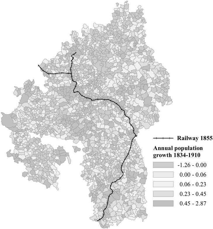
Figure 1 AVERAGE ANNUAL POPULATION GROWTH IN 1834–1910
Notes: The figure shows the average annual population growth in parishes in Württemberg between 1834 and 1910. The solid black line depicts the railway network in 1855.
Sources: Kunz and Zipf (Reference Kunz and Zipf2008), Dumjahn (Reference Dumjahn1984), Kommission für geschichtliche Landeskunde in Baden-Württemberg and Landesvermessungsamt Baden-Württemberg (1972), and Statistisches Landesamt Baden-Württemberg (2008). Authors’ design.
We digitized data on the average daily wage of day laborers (ortsübliche Tagelöhne gewöhnlicher Tagarbeiter) in 1884, 1898, and 1909, taxable income and building tax revenues in 1907, and the fire insurance value of buildings in 1908 (Königliches Statistisches Landesamt 1898, 1910). The wage data, recorded following the Sickness Insurance Law of 1883, distinguish between female and male workers. Taxable income refers to natural persons and equals income net of tax allowances and other deductions. We approximate average housing values from building tax revenues in 1907 and use average fire insurance values as an alternative indicator.Footnote 12
We further digitized employment data from the occupation censuses of 1895 and 1907 (Königliches Statistisches Landesamt 1900a, 1910),Footnote 13 which comprise parish-level information on the number of full-time gainfully employed persons (self-employed and dependent) in agriculture, industry, and trade and transport. We also digitized Württemberg’s Gewerbestatistik for 1829 (various volumes of Gewerbekataster, Staatsarchiv Ludwigsburg E 258 VI) and 1895 (Königliches Statistisches Landesamt 1900b).Footnote 14 Gewerbe includes mining, manufacturing, handicrafts, construction, trade, and transport (excluding railways and post). The data provide information on the number of establishments and their total employment, disaggregated by 3-digit sectors.Footnote 15 We use the Gewerbestatistik to distinguish between industrial employment in specific industries, measure specialization using the Herfindahl-Hirschman-Index (HHI),Footnote 16 16 and calculate the average number of persons employed in an establishment (Hauptbetrieb).
Finally, we obtain data on the location of steam engines from archival records (Staatsarchiv Ludwigsburg E 170 Bü 272). Data are available from 1845 to 1869 and include the year of installation and the maximum capacity of each steam engine.
RAILWAY ACCESS
We link the panel data on population, sectoral employment, and income with geo-referenced information on parishes and railway construction in Württemberg. Dumjahn (Reference Dumjahn1984) and Wolff and Menges (Reference Wolff and Menges1995) report the starting and end points of each railway line, the length of the line, and its opening date. We use this information to define the nodes of the railway network. We identify parishes as nodes if they served as network junctions or were the starting or end points of a railway segment that was constructed without interruption. Data on railway stations in 1911 are published in Königliches Statistisches Landesamt (1911).
CONTROL VARIABLES
We take information on the pre-railway share of Protestants from the Königliches Statistisches Landesamt (1824). We add data on the location of manufactories in 1832, published by Memminger (1833). Data on the average elevation of parishes come from the Bundesamt für Kartographie und Geodäsie (2017). We also add dummies for being located at a river navigable in 1845 and being connected to a paved road in 1848 (Kunz and Zipf Reference Kunz and Zipf2008).
EMPIRICAL STRATEGY
Treatment and Control Group
The main challenge in identifying the causal effect of railway access is that parishes were not randomly chosen to be connected to the railway. Table 1 illustrates this selection problem: It compares economic and demographic characteristics of different groups of parishes before the construction of Württemberg’s railway network began. Column (1) shows characteristics for the railway nodes, Column (2) for other parishes that gained access to the railway in the first stage of the railway expansion, and Column (3) for all other parishes. Columns (5) and (6) restrict attention to the sub-sample of winner and runner-up parishes.
Table 1 GROUP COMPARISON OF PRE-TREATMENT CHARACTERISTICS

Notes: The table shows average values of pre-treatment characteristics for nodes (Column (1)), railway parishes (Column (2)), and non-railway parishes (Column (3)), “winners” (Column (5)), and “runners-up” (Column (6)). Column (4) shows the mean difference in pre-treatment characteristics between railway and non-railway parishes and Column (7) the mean difference between winners and runners-up. Nodes are defined as parishes that are either starting or end points of a railway segment or serve as network junctions. Railway parishes obtained railway access in the first construction stage 1845–1854 (but are not nodes). Non-railway parishes did not obtain railway access in the first construction stage. Winners are parishes that obtained railway access in the first construction stage (but are not nodes). Runners-up are parishes that would have obtained railway access in the first construction stage if unrealized alternative routes had been built. Standard deviations are in parentheses (Columns (1)–(3) and (5)–(6)). Standard errors of a two-sided mean difference t-test are in brackets (Columns (4) and (7)).
Sources: Population in 1834 is from Statistisches Landesamt Baden-Württemberg (2008). The share of Protestants is from Königliches Statistisches Landesamt (1824). The location of manufactories in 1832 is from Memminger (1833). Industrial employment 1829 is from various volumes of Gewerbekataster (Staatsarchiv Ludwigsburg E 258 VI). Elevation is from Bundesamt für Kartographie und Geodäsie (2017). The locations of rivers navigable in 1845 and paved roads in 1848 are from Kunz and Zipf (Reference Kunz and Zipf2008).
Württemberg’s government generally chose the largest and economically most important cities—such as the capital Stuttgart—as railway nodes. Nodes had a much higher population than other parishes and were more likely to be located on rivers and to have a manufactory in 1832 (see Column (1) of Table 1). As it is common in the literature, our analysis excludes nodes and focuses on the effect of railway access on parishes that gained access to the railway in the first stage of the expansion (but were not nodes). These are the parishes in the treatment group.
One potential control group is all parishes that did not gain access to the railway in the first stage of the expansion. However, the selection problem carries over—albeit in muted form—to a comparison between railway parishes that were not nodes (Column (2)) and non-railway parishes (Column (3)). Treated parishes were generally larger, situated at lower altitudes, and more likely to have road access than non-railway parishes (Column (4)). Comparisons between the two groups might thus yield biased estimates.
Parts of our analyses thus focus on an alternative control group, consisting of parishes that would have obtained access to the railway if proposed alternative routes had been built. As described previously, Württemberg’s government first determined the nodes of the network and then instructed a railway commission and external experts to develop the exact route for a given railway. The experts typically came up with several proposals. We use these proposals to identify runner-up parishes, that is, parishes with designated railway access on an alternative line that was eventually not built in the first stage of the railway expansion.
Figure 2 shows the runner-up parishes (crosses), along with the winner parishes (points) and the railway nodes (stars). Colors mark all parishes that, under a specific proposal, would have received access to the railway. Henceforth, we refer to all potential routes suggested for one line as a “case.” Overall, there are seven such cases in the first construction stage (see Online Appendix Table A-4 for details). The decision for or against a specific route was mainly based on technical aspects. Political conflicts with neighboring countries also played a role (see the “Background” section). In contrast, local special interest groups had arguably only a little influence on the decision process, despite their generally powerful role in Württemberg’s politics and society. Their influence was limited by the strong role played by the government (Mann Reference Mann2006) and external experts (Mühl and Seidel Reference Mühl and Seidel1980) in the choice of network connections (Online Appendix 7 discusses these points at great length).
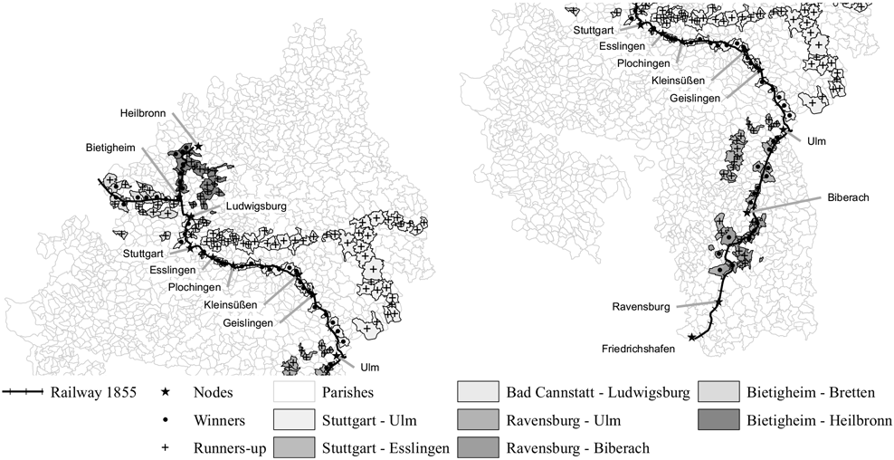
Figure 2 WINNER AND RUNNER-UP PARISHES
Notes: The figure shows railway nodes (stars), “winner parishes” (points), and “runner-up parishes” (crosses). The nodes are labeled in the map. Winners are parishes that obtained railway access in the first construction stage (but are not nodes). Runners-up are parishes with designated railway access on an alternative line that was eventually not built in the first stage of the railway expansion. Colors distinguish between the different cases and mark all potential routes suggested for one railway line. “Gaps” between winners or runners-up along a proposed route arise because not all parishes traversed by a railway line were (meant to be) connected to the railway.
Sources: Dumjahn (Reference Dumjahn1984), Etzel et al. (Reference Etzel, Klein and Knoll1985), Kunz and Zipf (Reference Kunz and Zipf2008), Kommission für geschichtliche Landeskunde in Baden-Württemberg and Landesvermessungsamt Baden-Württemberg (1972), and Königliches Statistisches Landesamt (1911). Authors’ design.
We rely on runner-up or losing parishes to identify a valid counterfactual for what would have happened to railway parishes had they not gained access to the railway in the first stage of the railway construction. Runner-up parishes should share many pre-treatment characteristics with parishes in the treatment group, as both groups were candidates for railway access in the first stage. In fact, many of the proposed lines that were initially not realized were built later.
Columns (5) to (7) of Table 1 provide support for our empirical strategy. Differences in pre-treatment characteristics decrease considerably when we compare the winner (Column (5)) and runner-up parishes (Column (6)).Footnote 17 This holds, in particular, for parishes’ access to roads and rivers, which differed greatly between railway and non-railway parishes but not between winner and runner-up parishes. In fact, none of the mean differences between winners and runners-up is statistically significantly different from zero (Column (7)) (although this may also be due to the small sample size). If anything, winners appear to be smaller and less industrialized than runners-up before the coming of the railway.
Distinguishing, in contrast, between parishes that are and are not located on a straight-line corridor between two railway nodes does not balance pre-treatment characteristics. Online Appendix Table A-10 shows that parishes on a straight-line corridor (or least cost path) were much more likely to have been connected to pre-railway transport networks. The significant differences in pre-treatment observables suggest that unobservables may also differ between groups. Using location on a straight-line corridor or least-cost path as an instrument for railway access, as done in most of the related literature, may produce biased estimates.Footnote 18
Empirical Specification
PANEL FIXED EFFECTS REGRESSION
We begin by estimating the effect of railway access using a standard two-way fixed effects regression, which we describe in the following for the comparison of winner and runner-up parishes. Let D ij,1855 be a binary treatment group indicator that indicates whether parish i along case j (a case comprises all potential routes suggested for one line) was connected to the railway by 1855, and let y ijt be an outcome variable in year t. Our baseline specification is:
 $$\matrix{
{{y_{ijt}}} \hfill & = \hfill & {{\theta _i} + {\lambda _t} + \beta {D_{ij,1855}} + \gamma \left( {{D_{ij,1855}} \times 1\left( {\tau \ge 0} \right){}_{jt}} \right) + {\varepsilon _{ijt}}} \hfill \cr
{} \hfill & = \hfill & {{\theta _i} + {\lambda _t} + \beta {D_{ij,1855}} + \gamma Lin{e_{ijt}} + {\varepsilon _{ijt}},} \hfill \cr
} $$
$$\matrix{
{{y_{ijt}}} \hfill & = \hfill & {{\theta _i} + {\lambda _t} + \beta {D_{ij,1855}} + \gamma \left( {{D_{ij,1855}} \times 1\left( {\tau \ge 0} \right){}_{jt}} \right) + {\varepsilon _{ijt}}} \hfill \cr
{} \hfill & = \hfill & {{\theta _i} + {\lambda _t} + \beta {D_{ij,1855}} + \gamma Lin{e_{ijt}} + {\varepsilon _{ijt}},} \hfill \cr
} $$
where θ i and λ t are parish and year fixed effects, respectively. τ denotes years but is normalized so that for each case, the railway line’s opening year is τ = 0. 1(τ ≥ 0) jt is thus a dummy equal to one for all years after case j’s railway line was opened. Opening years vary between 1843 and 1855.Footnote 19 The treatment variable Line ijt thus indicates whether a parish in the treatment group has railway access in year t.
The coefficient of interest (γ) captures mean shifts in outcome variables of treatment relative to control parishes after the railway line was opened. For most outcome variables (sectoral employment, specialization, firm size, adoption of steam), we have data for one year before (typically 1829) and one year after the first stage of the construction of the railway network (typically 1895/1907). This renders Equation (1) a standard differences-in-differences (DiD) equation with two groups (winners and runners-up) and two periods (before and after treatment). For population, we use data for 21 census years between 1834 and 1910.Footnote 20
Identification of the impact of the railway in Equation (1) rests on the assumption that parishes that gained access to the network until 1855 would have developed similarly to other parishes in the absence of railway construction. The similarity of treated and control parishes in their pre-railway outcomes (see Table 1) lends credibility to the assumption. We probe the robustness of our estimates with the inclusion of year-by-case fixed effects and test for differences in pre-treatment trends in our analysis of the effect of railways on the population size.
EVENT STUDY ANALYSIS
Specification (1) tests for a mean shift in our outcome variables. In our population analysis with many periods, the model implicitly assumes that any effect occurs immediately and then remains constant over time. In additional event study regressions, we relax this assumption and allow the effect to vary with the time since treatment by estimating:
 $$\matrix{
{{y_{ijt}}} \hfill & = \hfill & {{\theta _i} + {\lambda _t} + \ddot \beta {D_{ij,1855}} + \sum\nolimits_{k = - 4}^{13} {\gamma \left( {{D_{ij,1855}} \times 1\left( {\tau = k} \right){}_{jt}} \right)} } \hfill \cr
{} \hfill & = \hfill & {\sum\nolimits_{k = - 4}^{13} {{\delta _k}1{{\left( {\tau = k} \right)}_{jt}} + {{\ddot \varepsilon }_{ijt}}.} } \hfill \cr
} $$
$$\matrix{
{{y_{ijt}}} \hfill & = \hfill & {{\theta _i} + {\lambda _t} + \ddot \beta {D_{ij,1855}} + \sum\nolimits_{k = - 4}^{13} {\gamma \left( {{D_{ij,1855}} \times 1\left( {\tau = k} \right){}_{jt}} \right)} } \hfill \cr
{} \hfill & = \hfill & {\sum\nolimits_{k = - 4}^{13} {{\delta _k}1{{\left( {\tau = k} \right)}_{jt}} + {{\ddot \varepsilon }_{ijt}}.} } \hfill \cr
} $$
Coefficient γ k for k ≥ 0 corresponds to the difference in log population between treated and runner-up parishes k observation periods after the railway line was opened.Footnote 21 The difference is expressed relative to the four periods before the line was opened (i.e., we normalize γ –4 to zero).Footnote 22 We estimate the specification for –4 ≤ τ ≤ 13, as the sample is balanced for these periods. Specification (2) also tests for differences in trends between treated and control parishes in the periods before the railway line was opened.
SEMI-PARAMETRIC ESTIMATES
We can interpret the parameter γ in Equation (1) as an estimate of the average treatment effect on the treated (ATT). However, this interpretation hinges on the linearity assumption present in Equation (1). In an alternative strategy, we leave the data-generating process of the outcome variables unspecified and estimate the ATT by inverse probability weighting (IPW) (see Online >Appendix 9 for technical details). IPW estimates the ATT by comparing weighted outcome means of parishes with and without railway access. Intuitively, IPW places more weight on observations in the control group that—given their covariates—had a high probability of being treated in the first place.
The key assumption for IPW to yield the causal effect of interest is that, conditional on covariates, potential outcomes are independent of railway access. In contrast to DiD, IPW does not require data on the pre-treatment period, which we lack for agricultural employment, income, wages, and housing values. In a robustness check, we use the inverse probability weighted regression adjustment (IPWRA) approach, which has the advantage that either the outcome or the treatment model has to be correctly specified, not both (see Online Appendix 9). Estimating cross-sectional models by OLS rather than IPW or IPWRA yields very similar results.
Our covariates in IPW and IPWRA include log population and log population density in 1834, the share of protestants in 1821, a binary variable that indicates a running manufactory or factory in 1832, industrial employment per 100 persons in 1829, the average elevation in meters, and two binary variables that indicate access to a paved road in 1848 and a waterway navigable in 1845 (see Table 1 for summary statistics). We also add case-fixed effects as controls.
AVERAGE EFFECTS OF THE RAILWAY: WÜRTTEMBERG-WIDE RESULTS
Population Growth
Table 2 presents panel regression estimates of the effect of obtaining railway access in the first construction phase on the population size. Column (1) reports results from our baseline Specification (1) with year and parish fixed effects, restricting the sample to the winner and runner-up parishes. The regression suggests that railway access increased the population of winning parishes by 0.117 log points (relative to losing parishes). This effect is statistically significant, with a standard error of 0.033. Specification (2) adds year-by-case fixed effects, which control for case-specific time trends. Specification (3) adds a binary control variable that switches to one once a parish in the control group obtains railway access in the second or third construction phase. The estimated treatment effect increases only slightly to 0.136 (s.e. of 0.032) and 0.123 (s.e. of 0.026), respectively. Inference based on Conley standard errors, which account for potential spatial and serial correlation, yields very similar results (see Online Appendix Table A-8 for details).
Table 2 PANEL ESTIMATES OF THE EFFECT OF RAILWAY ACCESS ON POPULATION

* = Significant at the 1 percent level.
** = Significant at the 5 percent level.
*** = Significant at the 10 percent level.
Notes: The table shows panel regression estimates of the effect of railway access in 1845–54 on log population. Regressions (1) to (3) are estimated for the winners versus runners-up sample, regressions (4) to (6) for the complete sample excluding railway nodes. All regressions include a full set of year and parish dummies. Regressions (2) and (3) additionally include year-by-case fixed effects and regressions (5) and (6) include year-by-county (Oberamt) fixed effects. Regressions (3) and (6) add a time-varying control for railway access in later construction phases. Standard errors clustered at the parish level are in parentheses.
Sources: Population data are from Statistisches Landesamt Baden-Württemberg (2008).
Specifications (4) to (6) re-estimate the regressions on the full sample of parishes. At 0.172 (s.e. of 0.024), the baseline estimate for the full sample is larger than the corresponding estimate for the winners versus runners-up sample. This is consistent with the notion that in the full sample, the control group includes many small and remote parishes with unfavorable growth perspectives. The treatment effect in Column (4) is thus likely upward biased. The difference in the treatment effect estimated for the two samples vanishes when we add year-by-county fixed effects (Column (5)), which account for time-varying differences between Württemberg’s 64 counties (Oberämter).Footnote 23 Controlling for later railway access hardly affects the estimated treatment effect (Column (6)). Although the full-fledged panel model delivers similar results for both samples, we focus on the more comparable winners versus runners-up sample in what follows. This is because we cannot estimate panel models for the subset of outcomes that we observe only after the first stage of the railway expansion.
The event study analysis allows the effect of railway access on the population size to vary with time since treatment. Figure 3 shows the estimated differences in log population between the winner and runner-up parishes, relative to the baseline difference four periods before the treatment. Point estimates for the pre-treatment periods are very close to zero and statistically insignificant. Population in winning and losing parishes thus evolved in tandem before the arrival of the railway. At the time of the treatment, the point estimate jumps up to 0.036. The difference in log population then gradually widens with time since treatment. Thirteen periods after treatment or after about 50 years,Footnote 24 the population in winning parishes is, on average, 0.248 log points larger than in runner-up parishes. This corresponds to an increase in annual population growth of about 0.4 percentage points.
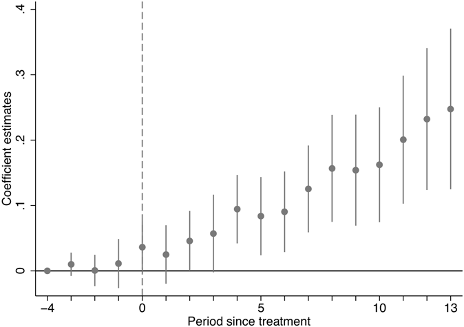
Figure 3 EVENT STUDY ESTIMATES OF THE EFFECT OF RAILWAY ACCESS ON LOG POPULATION
Notes: The graph depicts differences in log population between winner and runner-up parishes for pre- and post-treatment periods, as estimated in an event study regression. Differences are expressed relative to the baseline difference four periods before the treatment. Point estimates are marked by a dot. The vertical bands indicate the 95 percent confidence interval of each estimate. The dashed vertical line indicates the treatment period.
Sources: Population data are from Statistisches Landesamt Baden-Württemberg (2008).
Several additional results for the impact of the railway on population and demographic change are shown in the online appendices. Online Appendix 11 documents that semi-parametric IPW and IPWRA yield results that are almost identical to the event study estimates. This is reassuring for our subsequent analyses of wages, income, and housing values, which are based on cross-sectional estimates only due to the lack of pre-treatment data. Online Appendix 12 presents event study and semi-parametric estimates for the full sample, which are similar to those for the winners versus runners-up sample.
Online Appendix 13 presents evidence that the railway increased parish-level population by attracting immigration rather than increasing fertility, in line with earlier results for Prussia (Hornung Reference Hornung2015). Workers arguably moved into railway parishes in search of higher wages and employment opportunities in industry, consistent with spatial equilibrium models.Footnote 25
Online Appendix 14 shows for the full sample of parishes that gaining access in the second stage from 1857 to 1886 also boosted population.Footnote 26 However, the effect of the second stage is somewhat smaller than the first. This is not surprising, as the most important lines, especially for transit passengers and freight, have already been built in the first construction phase. The difference in effect size also cautions against extrapolating from the effects of the main railway lines to the effects of the railway network at large.
We also study whether the positive effects near the railway come at the expense of locations in middle distances. Estimates from local polynomial regressions yield little evidence for localized displacement effects in our finely grained spatial data. Online Appendix 15 discusses these results in more detail.
Income, Wages, and Housing Values
We next analyze the effect of railway access on income, wages, and housing values. In spatial equilibrium, we would expect population increases to go hand in hand with increases in income and housing values. We focus on the more comparable parishes in the winners versus runners-up sample and report qualitatively similar findings for the full sample in Online Appendix 19.Footnote 27
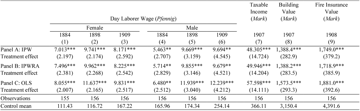
We first consider the effect of railway access on the average daily wage of day laborers in 1884, 1898, and 1909, distinguishing between females and males (see Columns (1) to (6) in Table 3). Estimates from IPW (Panel A), IPWRA (Panel B), and OLS (Panel C) models all suggest that railway access had a statistically significant positive wage effect. IPW estimates indicate that access increased female day laborer wages by 7.0, 9.7, and 8.2 Pfennig in 1884, 1898, and 1909, respectively. This corresponds to an increase of 6.3, 8.3, and 4.9 percent, respectively, relative to the control group average. The relative effect is somewhat lower for male day laborers, ranging from 3.3 to 5.5 percent. These results suggest that railway-induced industrialization also benefited the working class.Footnote 28 The higher treatment effect for females translates into a statistically significant lower gender wage gap in winning parishes of 2.0 and 1.7 percentage points in 1884 and 1898, respectively (from a baseline of 32.8 percent). See Online Appendix Table A-9 for details. The lower gender wage gap is consistent with the idea that falling transport costs induced mechanization, which in turn increased the relative productivity of women by reducing the importance of human strength in production (Goldin Reference Goldin1990; Galor and Weil Reference Galor and Weil1996).
Table 3 THE EFFECT OF RAILWAY ACCESS ON DAY LABORER WAGES, TAXABLE INCOME, AND BUILDING VALUES
* = Significant at the 10 percent level.
** = Significant at the 5 percent level.
*** = Significant at the 1 percent level.
Notes: The table shows regression estimates of the effect of railway access in 1845–54 on the average daily wage of female (Columns (1) to (3)) and male (Columns (4) to (6)) day laborers in 1884, 1898, and 1909, on taxable income per capita in 1907 (Column (7)), the average value of buildings in 1907 (Column (8)), and the average fire insurance value per building in 1908 (Column (9)). Values in Columns (1) to (6) are in Pfennig and values in Columns (7) to (9) are in Mark, with 1 Mark = 100 Pfennig. Regressions in Panel A are estimated by IPW, regressions in Panel B by IPWRA and regressions in Panel C by OLS. All regressions include as control variables log population and log population density in 1834, the share of protestants in 1821, a dummy for having a manufactory in 1832, industry employment per 100 persons in 1829, elevation, dummies for access to a navigable river in 1845 and to a road in 1848, and case dummies. Robust standard errors are in parentheses.
Sources: The average daily wage of day laborers in 1884, 1898, and 1909, taxable income and building value in 1907, and the fire insurance value of buildings in 1908 are from Königliches Statistisches Landesamt (1898, 1910).
We next consider taxable income per capita in 1907. The IPW estimate suggests that railway access increased the annual taxable income in winning parishes by 48.3 Mark or 13.2 percent (see Column (7) of Table 3). The relative increase in taxable income is thus comparable to the increase in day-laborer wages. Finally, Columns (8) and (9) of Table 3 show the treatment effect on the average building value in 1907 and the fire insurance value in 1908, respectively. Railway access increased the average building value by 1,388.4 Mark or 44.1 percent (IPW estimate in Panel A). The increase in insurance value per building is of comparable size.
Industrial Development and Sectoral Employment
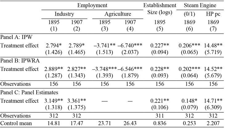
We next study the effect of railway access on structural change from agriculture to industry, a core characteristic of the Industrial Revolution. We also provide evidence on specific sectors identified in the literature as drivers of Germany’s industrialization process. We again focus on the winners versus runners-up sample and report qualitatively similar results for the full sample in Online Appendix 19>. We first study the effect of railway access on various measures of industrial development. Panels A and B of Table 4 present results from IPW and IPWRA estimations and Panel C from DiD regressions. Columns (1) to (4) show that railway access accelerated the transition from agriculture to industry. The IPW estimates in Column (1) of Panel A imply that railway access increased industry employment in winning parishes by 2.8 employees per 100 persons or 18.9 percent relative to the 1895 average in losing parishes. The percent increase in industrial employment in 1907 (Column (2)) is similar to that in 1895. Increased industrial employment came at the expense of agricultural employment (Columns (3) and (4)). The IPW estimate implies that railway access decreased the number of full-time employees in agriculture by 3.7 employees per 100 persons in 1895, or 15.8 percent relative to the control group average. This negative effect increases to 6.7 employees or 25.5 percent in 1907.Footnote 29 The results of the IPWRA (Panel B) and DiD regressions (Panel C) are almost identical to the IPW estimates.
Table 4 THE EFFECT OF RAILWAY ACCESS ON INDUSTRIAL DEVELOPMENT
* = Significant at the 10 percent level.
** = Significant at the 5 percent level.
*** = Significant at the 1 percent level.
Notes: The table shows estimates of the effect of railway access in 1845–54 on the number of full-time employees in industry (Columns (1) and (2)) and agriculture (Columns (3) and (4)) per 100 persons in 1895 and 1907, establishment size in industry in 1895 (Column (5)), the probability of having installed at least one steam engine by 1869 (Column (6)), and steam horsepower per 1,000 persons in 1869 (Column (7)). Panels A and B display IPW and IPWRA estimates, respectively. Regressions in Panels A and B include as control variables log population and log population density in 1834, the share of protestants in 1821, a dummy for having a manufactory in 1832, elevation, dummies for access to a navigable river in 1845 and to a road in 1848, and case dummies. Panel C displays estimates from panel fixed effects regression that include parish and year-by-case fixed effects. The pre-treatment period is 1829 in Columns (1) to (5) and 1846 in Columns (6) and (7). We cannot run panel fixed effects regression for agricultural employment, as we lack data for the pre-treatment period. The control mean gives the mean value of the outcome for the control group in 1895 (Columns (1), (3), (5)) 1907 (Columns (2) and (4)), and 1869 (Columns (6) and (7)). Robust standard errors are in parentheses. Standard errors in Panel C are clustered at the parish level.
Sources: Employment data are from the occupation censuses of 1895 and 1907 (Königliches Statistisches Landesamt 1900a, 1910), the Gewerbestatistik of 1829 (various volumes of Gewerbekataster, Staatsarchiv Ludwigsburg E 258 VI), and 1895 (Königliches Statistisches Landesamt 1900b). Data on the location of steam engines are from archival records (Staatsarchiv Ludwigsburg E 170 Bü 272).
Falling transport costs are widely believed to have increased optimal establishment size by integrating markets and expanding market size. The ensuing competitive pressures, so the argument goes, forced firms to increase productivity through the division of labor and mechanization and thus promoted the rise of factories (Atack, Haines, and Margo Reference Atack, Haines, Margo, Paul, Joshua and David2011). In line with this argument, we find that railway access increased establishment size by between 0.221 and 0.228 log points compared to losing parishes (Column (5) of Table 4).
We also find strong evidence that the railway accelerated local technological change. IPW/ IPWRA estimates suggest that railway access increased the likelihood of having at least one steam engine in operation in 1867 by more than 20 percentage points (from a baseline of 25.3 percent in losing parishes) and the total steam power installed by 14.5 horsepower per 1,000 persons (from a baseline of 2.2). Railway access lowered the costs of coal shipments sufficiently for steam-powered industrial growth to happen outside the coal mining regions (Gutberlet Reference Gutberlet2014).
Our unusually disaggregated data allow us to study the employment effect of railways on specific industries. Table 5 shows results from IPW (Panel A), IPWRA (Panel B), and DiD (Panel C) models. Column (1) suggests that railway access boosted the local textile industry, Württemberg’s most important industry at the dawn of the Industrial Revolution. Average 1895 employment in the textile sector (excluding fiber production) was 4.3 employees per 100 persons in winning parishes but only 2.0 employees in losing parishes. In contrast, textile employment was virtually identical in the pre-treatment period of 1829 (1.9 and 2.0 in winning and losing parishes, respectively). The railway expanded the market for textile exports and enabled coal to be transported to power steam engines. In fact, the textile industry used 37.8 percent of the steam power installed in Württemberg in 1875 (Kaiserliches Statistisches Amt 1879).
Table 5 THE EFFECT OF RAILWAY ACCESS ON EMPLOYMENT IN KEY INDUSTRIAL SECTORS AND SPECIALIZATION

* = Significant at the 10 percent level.
** = Significant at the 5 percent level.
*** = Significant at the 1 percent level.
Notes: The table shows estimates of the effect of railway access in 1845–54 on the number of full-time employees per 100 persons in different industries (Columns (1)–(5)) and specialization within industry (Column (6)) in 1895. We distinguish between employment in the textile industry (Column (1)), coal, iron, and steel industry (Column (2)), building of machines and instruments (Column (3)), building of electrical machines and instruments (Column (4)), and the chemical industry (Column (5)). Specialization is measured by the Hirschman-Herfindahl-Index (with a = 2). Panels A and B display IPW and IPWRA estimates, respectively, using employment in 1895 as outcome variable. Regressions in Panels A and B include as control variables log population and log population density in 1834, industry employment per 100 persons in 1829, a dummy for having a manufactory in 1832, the share of protestants in 1821, elevation, dummies for access to a navigable river in 1845 and to a road in 1848, and case dummies. Panel C displays estimates from panel fixed effects regression that include parish and year-by-case fixed effects. The pre-treatment period is 1829. The control mean gives the mean value of the outcome for the control group in 1895. Robust standard errors, clustered at the parish level in Panel C, are in parentheses.
Sources: Employment data are from the Gewerbestatistik of 1829 (various volumes of Gewerbekataster, Staatsarchiv Ludwigsburg E 258 VI) and 1895 (Königliches Statistisches Landesamt 1900b).
In contrast, the railway did not increase employment in the coal, iron, and steel industries, which played a core role in Germany’s growth take-off during the third quarter of the nineteenth century (Broadberry, Fremdling, and Solar Reference Broadberry, Fremdling and Solar2008; Ziegler Reference Ziegler2012). If anything, the effect is negative (though not statistically significant, see Column (2)). This result might seem surprising, as railways boosted German coal, iron, and steel production (Fremdling Reference Fremdling1985). However, Württemberg lacked coal deposits. After the railway markedly decreased transport costs, Württemberg’s steel and iron producers were no longer able to compete with the cheaper producers located in the resource-rich Ruhr and Saar regions. Consequently, Württemberg’s share in the German pig iron and steel production plummeted from 2.6 percent in 1850 to 0.2 percent around 1895 (von Hippel 1992). Online Appendix 16 documents and discusses the decline of iron producers across Württemberg between 1834 and 1895 in greater detail.
Column (3) shows that railway access strongly increased employment in the machine and instrument building industry (by about 0.5 employees per 100 persons from a baseline of 0.1 employees), which was an important driver of economic growth in Germany both during the earlier and later stages of the Industrial Revolution. The drive towards mechanization and the expansion of the railway were pivotal for the rise of Württemberg’s machine and instrument industry since the mid-nineteenth century (von Hippel 1992). In fact, Württemberg’s largest industrial company at the time, the Maschinenfabrik Esslingen, was founded in 1846 to produce locomotives for Württemberg’s public railway company.Footnote 30 Since Württemberg’s machine industry was export-oriented, it also benefited from the falling transport costs brought about by the railway.
The late nineteenth century saw the rise of the electronic and chemical industries in Germany, which gradually replaced heavy industry as the leading sector in Germany’s industrialization process. However, both industries were still small in Württemberg in 1895, counting 821 (electronic) and 2,232 (chemical, excluding pharmacies) employees in the entire state. Columns (4) and (5) show that railway access is positively associated with employment in the two industries, but the estimates are small and not statistically significant.
Finally, Column (6) in Table 5 reports evidence that the degree of specialization within industry is lower in winning than in losing parishes. However, the estimates are imprecise and not statistically significant at conventional levels.
HETEROGENEOUS EFFECTS OF THE RAILWAY
This section tests whether the effects of gaining railway access in the first construction phase were larger for parishes that already had a manufactory in 1832 and for those with an above-median population in 1843,Footnote 31 in line with arguments in Gutberlet (Reference Gutberlet2013) and Ziegler (Reference Ziegler2012). As the railway decreased transport costs, we might expect that agglomeration forces drew industrial economic activity to the more populous centers (Krugman Reference Krugman1991). Consequently, these centers experienced a disproportionate increase in population and industrial employment. Regional agglomeration drove up nominal wages but also led to higher housing prices (e.g., Südekum Reference Südekum2008).Footnote 32 Since the analyses are demanding on the data, we focus on the full sample of parishes. Results based on the winners versus runners-up sample are qualitatively similar.
Table 6 studies heterogeneity in the effect of railway access on the population. We estimate DiD specifications with parish and year-by-county fixed effects. Since the event study analysis has shown that the treatment effect grows over time, we estimate a linear trend break instead of a constant treatment coefficient (Goodman-Bacon Reference Goodman-Bacon2021). The linear time break specification interacts the treatment dummy Line ijt in Equation (1) with the difference between year t and the year a line was opened (plus one). We focus on a panel setup with a trend-break treatment rather than the event study model to reduce complexity. The estimate in Column (1) implies that railway access increased annual population growth by, on average, 0.6 percentage points.
Table 6 HETEROGENEOUS EFFECTS OF RAILWAY ACCESS ON POPULATION, DiD ESTIMATES

* = Significant at the 10 percent level.
** = Significant at the 5 percent level.
*** = Significant at the 1 percent level.
Notes: The table shows panel regression estimates of the effect of railway access in 1845–54 on log population, based on the full sample excluding railway nodes (38,766 observations). We assume that the treatment effect is a linear time break. Thus, we interact Line ijt in Equation (1) with the difference between year t and the year a line was opened (plus one). All regressions include a full set of parish dummies and year-by-county fixed effects. Regressions (2)–(3) add interaction terms between the treatment (linear time break) and pre-railway parish characteristics, namely the existence of a manufactory in 1832 (regression (2)) and above-median population in 1843 (regression (3)). Standard errors clustered at the parish level are in parentheses.
Sources: Population data are from Statistisches Landesamt Baden-Württemberg (2008).
The remaining specifications add interactions between the trend break and dummies for having a manufactory in 1832 and above-median population in 1843. Column (2) shows that the positive effect of railway access on population is more than twice as large for parishes that already had a manufactory in 1832 (1.2 percentage points relative to a baseline effect of 0.5 points for parishes without a manufactory). This is consistent with the prediction that industrial centers particularly benefited from the railway-induced increase in market access. Moreover, the effect of railway access on annual population growth is 0.5 percentage points higher in larger than in smaller parishes (Column (3)). Thus, the railway reinforced pre-existing population differences. This finding is in line with recent evidence for England and Wales (Bogart et al. Reference Bogart, Xuesheng You, Satchell and Shaw-Taylor2022).
Columns (1) to (5) of Table 7 test for heterogeneity in the effect of railway access on wages, income, and housing values. Panel A reports average effects, whereas Panels B and C report heterogeneous effects. We interact the treatment dummy with the relevant parish characteristics, which we also include as controls in our (cross-sectional) regressions. As expected, the results mirror our findings for population. We find that the positive effects of railway access on wages, income, and housing values are two to three times larger for parishes that already had a manufactory in 1832 (Panel B of Table 7), although differences in effect size are relatively imprecisely estimated, especially for income and building values. Effect heterogeneity by population (Panel C) is also sizable but tends to be smaller than by manufactory location.
Table 7 HETEROGENEOUS EFFECTS OF RAILWAY ACCESS ON DAY LABORER WAGES, TAXABLE INCOME, BUILDING VALUES, AND INDUSTRIAL DEVELOPMENT

* = Significant at the 10 percent level.
** = Significant at the 5 percent level.
*** = Significant at the 1 percent level.
Notes: The table shows heterogeneity in the effect of railway access in 1845–54 on the average daily wage of female (Column (1)) and male (Column (2)) day laborers in 1909, on taxable income per capita in 1907 (Column (3)), the average value of buildings in 1907 (Column (4)), the average fire insurance value per building in 1908 (Column (5)), the number of full-time employees in industry per 100 persons in 1907 (Column (6)), establishment size in industry in 1895 (Column (7)), the probability of having installed at least one steam engine by 1869 (Column (8)), and steam horsepower per 1,000 persons in 1869 (Column (9)). Estimates in Columns (1) to (5) are from cross-sectional OLS regressions on the full sample. Control variables include log population and log population density in 1834, the share of protestants in 1821, a dummy for having a manufactory in 1832, industry employment per 100 persons in 1829, elevation, dummies for access to a navigable river in 1845 and to a road in 1848, a dummy indicating whether population in the main location of residence in 1843 was above the treatment group median, and dummies for geographic location within Württemberg. Estimates in Columns (6) to (9) are from panel fixed effects regressions that include parish and year-by-county fixed effects. Regressions in Panel (A) report average effects of railway access. Regressions in Panels (B) and (C) add interaction terms between the treatment effect dummy and (pre-railway or time-invariant) parish characteristics, namely the existence of a manufactory in 1832 (Panel (B)) and above-median treatment group population in 1843 (Panel (C)). Robust standard errors, clustered at the parish level in Columns (6) to (9), are in parentheses.
Columns (6) to (9) of Table 7 study heterogeneity in the effect of railway access on industrial development, using panel regressions. We find that railway access had much stronger positive effects on industrial development in parishes that had a manufactory in 1832 (Panel B). For instance, the estimated effect on industry employment in 1895 was more than twice as large for parishes with a manufactory than for those without one (12.2 versus 5.2 employees per 100 persons). Likewise, the effect of railway access on establishment size is three times greater in manufactory parishes. Effect heterogeneity is even more pronounced in the adoption of steam.Footnote 33
Railway access also had stronger positive effects on industrial development in larger than smaller parishes (Panel C). Overall, the railway boosted industrial development, especially in existing industrial centers, thereby increasing the concentration of industrial activity.
Online Appendix 17> documents significant heterogeneity also by railway line. Parishes along the eastern and northern lines, which served Württemberg’s densely populated Neckar basin, benefited considerably more from the railway than parishes along the southern line, which served the sparsely populated southeast. This finding is consistent with our result that the railway benefited disproportionally larger and more industrial parishes. These parishes were concentrated in the Neckar basin even before the coming of the railway (Feyer Reference Feyer1973).
DISCUSSION AND CONCLUDING REMARKS
This paper has provided a comprehensive analysis of the average and heterogeneous effects of railway access on local growth and industrialization in Württemberg during the Industrial Revolution. Figure 4 summarizes our key findings. It depicts differences in log population between railway and non-railway parishes in 1834–1910, both for average railway parishes and for those with a manufactory in 1832. As a point of comparison, we also show how differences in population would have evolved had railway access increased annual growth by 1–2 percentage points, as was found for Prussian towns (Hornung Reference Hornung2015).
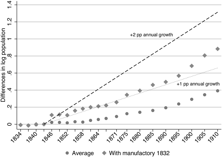
Figure 4 DIFFERENCES IN LOG POPULATION BETWEEN RAILWAY AND NON-RAILWAY PARISHES, 1834–1910
Notes: The graph depicts differences in log population between railway and non-railway parishes in 1834–1910, as estimated in panel regressions with parish and year-by-county fixed effects. The large dots mark the average growth estimate, diamonds those estimated for railway parish that had a manufactory in 1832. Estimates are based on the full sample, excluding railway nodes. 1843 serves as the baseline period. The black dotted and dashed lines show how differences in log population would have evolved if railway access had increased annual population growth by 1 and 2 percentage points, respectively.
Sources: Population data are from Statistisches Landesamt Baden-Württemberg (2008).
The figure illustrates that our estimates for population growth in Württemberg are considerably smaller than earlier estimates for Prussia. Large dots show that, initially, parishes that gained access to the railway in the first construction stage grew only modestly faster than parishes that did not. If we consider the period until 1871, as Hornung (Reference Hornung2015) does, railway access increased annual parish-level population growth in Württemberg by just 0.3 percentage points. In light of the core role ascribed to the railway in Germany’s industrialization process (Fremdling Reference Fremdling1977; Ziegler Reference Ziegler2012), the comparably small growth effects might partly explain why Württemberg was still relatively poor by German standards in the early twentieth century. The growth-enhancing effect of the railway was simply larger in other parts of Germany.
Why did Württemberg benefit less from the railway than Prussia? A first explanation is the belated construction of Württemberg’s railway network and its limited length. In Prussia, 21 railway lines were built in 1838–1848, connecting major cities such as Berlin and Hamburg or Magdeburg and Leipzig. In contrast, Württemberg’s railway network was limited to short sections around Stuttgart in 1848. This delayed construction of the railway network has been put forward as a potential cause for Württemberg’s late industrialization (Naujoks Reference Naujoks1982).
Württemberg’s railway network then gradually expanded in the second half of the nineteenth century. By 1868, the density of the railway network was higher in Württemberg than in Prussia (see Online Appendix Figure A-4 for a comparison of network density in Bavaria, Prussia, and Württemberg in 1848–1903). This might explain why the growth effects of early railway access increased over time, as also shown in Figure 4. Parishes along the main railway lines increasingly benefited from the growing network’s positive externalities.
However, positive network externalities were presumably smaller in Württemberg than in Prussia, as the latter had a much larger network. Although the railway networks of the different German states were connected, the railway administrations were not unified before 1920. This caused significant frictions in the railway traffic between German states, as timetables lacked coordination and price systems differed even after the foundation of the German Empire in 1871 (Ziegler Reference Ziegler2012). Without a comprehensive integration of the German railway network, positive externalities were presumably the largest in the dominant Prussian network.
Our finding of strong heterogeneity in the effect of railway access provides a second explanation for why we observe small average growth effects in Württemberg. Figure 4 illustrates that the effect of railway access on population growth was much stronger in parishes that had a manufactory in 1832. For them, growth effects were well within the 1–2 percentage points range reported for Prussia. Yet, only a very few parishes in Württemberg had a manufactory in the pre-railway era. This relative backwardness might have limited the railway’s overall growth effect. Württemberg lacked the industrial and coal-mining regions that benefited most from the interplay between railway and heavy industries in Germany (Gutberlet Reference Gutberlet2013; Ziegler Reference Ziegler2012).
The lack of coal limited backward linkages from the railway (Megerle Reference Megerle, Fremdling and Richard1979), which were decisive for the dramatic growth of Prussia’s coal, iron, and steel sectors. Württemberg’s iron producers could not compete with the cheap imports of coke pig iron from the Ruhr and Saar regions as transport costs decreased. Hence, Württemberg’s share of German iron and steel production plummeted in the second half of the nineteenth century, while Prussia’s share increased.
Our finding of significant effect heterogeneity is also important in its own right. The railway was not only an essential driver of Germany’s industrialization process. It also increased regional economic disparities between and within German states. This aspect remains under-explored in the literature on the railway’s impact on economic growth in nineteenth-century Germany. More generally, our findings show that investment in transportation infrastructure can have markedly different effects on growth and development depending on the specific local conditions. A better understanding of this heterogeneity can increase the effectiveness and efficiency of infrastructure investments in contemporary contexts. Our findings caution that transport infrastructure improvements might deepen regional inequality, often against the intention of policymakers.


 Open access