Weighted estimates for the multilinear maximal operator

Abstract

The paper contains the study of the weighted $L^{p_1}\times L^{p_2}\times \ldots \times L^{p_m}\rightarrow L^p$ estimates for the multilinear maximal operator, in the context of abstract probability spaces equipped with a tree-like structure. Using the Bellman function method, we identify the associated optimal constants in the symmetric case $p_1=p_2=\ldots =p_m$, and a tight constant for remaining choices of exponents.

1 Introduction

The purpose of this paper is to study a class of weighted inequalities for the multilinear maximal operator, an important object in harmonic analysis. We will be particularly interested in the size of the constants involved. To present the results from an appropriate perspective, let us start with the necessary background. Fix a dimension N and suppose that $\mathscr {D}$ is the standard dyadic lattice in $\mathbb {R}^N$. Let M be the dyadic maximal operator, acting on locally integrable functions f on $\mathbb {R}^N$ by

$$\begin{aligned} Mf(x)=\sup _{Q\in \mathscr {D}} \langle |f|\rangle _Q\chi _Q. \end{aligned}$$

Here the symbol $\langle \varphi \rangle _Q$ stands for the average of $\varphi$ over Q, calculated with respect to the Lebesgue measure: $\langle \varphi \rangle _Q =\frac{1}{|Q|}\int _Q \varphi$. Maximal operators play a prominent role in many areas of mathematics, and from the viewpoint of applications, it is often of interest to study the boundedness properties of these objects, treated as operators on various function spaces. A fundamental example is the sharp estimate

$$\begin{aligned} \Vert Mf\Vert _{L^p}\le p'\Vert f\Vert _{L^p},\qquad 1<p\le \infty \end{aligned}$$

(1)

(here and below, $p'$ denotes the conjugate exponent to p, given by $p'=p/(p-1)$). One can investigate numerous generalizations of this result, our motivation comes from an extension to the weighted theory. In what follows, the word ‘weight’ refers to a positive and locally integrable function on $\mathbb {R}^N$. Any weight w gives rise to the corresponding Borel measure, also denoted by w, and given by $w(A)=\int _A w\text{ d }x$. One can also introduce the associated weighted $L^p$ spaces, defined as the classes of all (equivalence classes of) functions $f:\mathbb {R}^N\rightarrow \mathbb {R}$ for which

$$\begin{aligned} \Vert f\Vert _{L^p(w)}:=\left( \int _{\mathbb {R}^N}|f|^pw\text{ d }x\right) ^{1/p}<\infty , \qquad 0<p<\infty . \end{aligned}$$

Now one can study the following problem related to (1): given $1<p<\infty$, characterize those weights w, for which the dyadic maximal operator M is bounded as an operator on $L^p(w)$. This problem was solved by Muckenhoupt [8] in the seventies: the boundedness is true if and only if w satisfies the so-called dyadic $A_p$ condition (or w belongs to the dyadic $A_p$ class). The latter means that the quantity

$$\begin{aligned}{}[w]_{A_p}:=\sup _{Q\in \mathscr {D}} \langle w\rangle _Q \langle \sigma \rangle _Q^{p-1}, \end{aligned}$$

called the $A_p$ characteristic of w, is finite. Here $\sigma =w^{1-p'}$ is the dual weight to w. There is a stronger, quantitative version of this result, established by Buckley at the beginning of the nineties. Namely, the problem is to find, for any fixed $1<p<\infty$, the least exponent $\beta (p)$ such that

$$\begin{aligned} \Vert M\Vert _{L^p(w)\rightarrow L^p(w)}\le \kappa _p [w]_{A_p}^{\beta (p)}, \end{aligned}$$

(2)

where $\kappa _p$ depends only on p. In other words, one is interested in the extraction of the optimal dependence of $\Vert M\Vert _{L^p(w)\rightarrow L^p(w)}$ on the $A_p$ characteristic $[w]_{A_p}$. The aforementioned result of Buckley [1] asserts that the optimal choice is given by $\beta (p)=(p-1)^{-1}$. This statement can be further improved: we need some additional notation for the further discussion. Given $1<p<\infty$ and $c\ge 1$, let $d=d(p,c)$ be the unique positive root of the equation

$$\begin{aligned} c(1+d)(p-1-d)^{p-1}=(p-1)^{p-1}. \end{aligned}$$

(3)

This parameter has a nice geometric interpretation: see Fig. 1 below.

Fig. 1

The tangent to the curve $xy^{p-1}=c$ at the point $(1,c^{1/(p-1)})$ intersects the curve $xy^{p-1}=1$ at $(1+d,(1+d)^{1/(p-1)})$

The paper [9] contains the proof of the following extension of Buckley’s result.

Theorem 1.1

For any $1<p<\infty$ we have the inequality

$$\begin{aligned} \Vert M\Vert _{L^p(w)\rightarrow L^p(w)}\le \frac{p}{p-1-d(p,[w]_{A_p})}. \end{aligned}$$

The constant on the right is the best possible: for any $c\ge 1$ and $\varepsilon >0$ there is an $A_p$ weight w satisfying $[w]_{A_p}\le c$ such that

$$\begin{aligned} \Vert M\Vert _{L^p(w)\rightarrow L^p(w)}\ge \frac{p}{p-1-d(p,c)}-\varepsilon . \end{aligned}$$

In our considerations below, we will be interested in the multilinear analogues of the above theorem. Suppose that $m\ge 1$ is a fixed integer. Following [5], the m-linear dyadic maximal operator $\mathcal {M}$ acts on vectors $\vec {f}=(f_1,f_2,\ldots ,f_m)$ of locally integrable functions on $\mathbb {R}^N$ by the formula

$$\begin{aligned} \mathcal {M}\vec {f}=\sup _{Q\in \mathscr {D}} \prod _{j=1}^m \langle |f_j|\rangle _Q\chi _Q. \end{aligned}$$

A straightforward combination of (1) and the Hölder inequality implies that if $\vec {P}=(p_1,p_2,\ldots ,p_m)$ is a sequence of exponents satisfying $1<p_1,p_2,\ldots ,p_m\le \infty$ and $\frac{1}{p}=\frac{1}{p_1}+\frac{1}{p_2}+\ldots +\frac{1}{p_m},$ then we have the sharp bound

$$\begin{aligned} \Vert \mathcal {M}\vec {f}\Vert _{L^p}\le \prod _{j=1}^m p_j'\Vert f_j\Vert _{L^{p_j}}. \end{aligned}$$

One can ask about the weighted version of this estimate, motivated by the above discussion for M. The precise answer was given by Lerner et al.  [5]. Given a vector $\vec {w}=(w_1,w_2,\ldots ,w_m)$ of weights on $\mathbb {R}^N$, we set

$$\begin{aligned} v_{\vec {w}}=\prod _{j=1}^m w_j^{p/p_j} \end{aligned}$$

and say that $\vec {w}$ satisfies the dyadic multilinear condition $A_{\vec {P}}$, if

$$\begin{aligned}{}[\vec {w}]_{A_{\vec {P}}}:=\sup _{Q\in \mathscr {D}} \langle v_{\vec {w}}\rangle _Q \prod _{j=1}^m \langle \sigma _j\rangle _Q^{p/p_j'}<\infty . \end{aligned}$$

Here, as before, $\sigma _j=w_j^{1-p_j'}$ is the dual weight to $w_j$, $j=1,\,2,\,\ldots ,\,m$. Note that for $m=1$, the above requirement reduces to the classical Muckenhoupt’s condition $A_p$. Actually, the connection to the one-dimensional setting goes deeper: as proved in [5], we have $\vec {w}\in A_{\vec {P}}$ if and only if $\sigma _j\in A_{mp_j'}$ for all j and $v_{\vec {w}}\in A_{mp}$. The multilinear $A_{\vec {P}}$ condition provides us with the answer to the above question: $\mathcal {M}$ is bounded as an operator from $L^{p_1}(w_1)\times L^{p_2}(w_2)\times \ldots \times L^{p_m}(w_m)$ to $L^p(v_{\vec {w}})$ if and only if $\vec {w}\in A_{\vec {P}}$. In [3], the authors established the following version of (2):

$$\begin{aligned} \Vert \mathcal {M}\vec {f}\Vert _{L^p(v_{\vec {w}})}\le \kappa _{\vec {P}}[\vec {w}]_{A_{\vec {P}}}^{\beta (\vec {P})} \prod _{j=1}^m \Vert f_j\Vert _{L^{p_j}(w_j)}, \end{aligned}$$

(4)

with $\beta (\vec {P})$ satisfying $\frac{m}{mp-1}\le \beta (\vec {P}) \le \frac{1}{p}\left( 1+\sum _{j=1}^m \frac{1}{p_j-1}\right)$. Furthermore, in the special case $p_1=p_2=\ldots =p_m=mp$, they showed that the estimate holds with $\beta (\vec {P})=m/(mp-1)=p_1'/p$, which is optimal. The question about the best exponent for an arbitrary vector $\vec {P}$ was answered in [6]: the optimal choice is $\beta (\vec {P})=\max \left\{ {p_1'}/{p},{p_2'}/{p},\ldots ,{p_m'}/{p}\right\} .$

The purpose of this paper is to present a different approach to the estimate (4), which will yield the further information about the size of the constant $\kappa _{\vec {P}}$. In addition, it will allow us to identify the best constant in the special case $p_1=p_2=\ldots =p_m=mp$. Actually, we will work in the more general context of probability spaces equipped with a tree-like structure. Here is the precise definition (cf. [7]).

Definition 1.2

Suppose that $(X,\mu )$ is a nonatomic probability space. A set $\mathcal {T}$ of measurable subsets of X will be called a tree if the following conditions are satisfied:

• (1) $X\in \mathcal {T}$ and for every $Q\in \mathcal {T}$ we have $\mu (Q)>0$.

• (2) For every $Q \in \mathcal {T}$ there is a finite subset $C(Q) \subset \mathcal {T}$ containing at least two elements such that (a) the elements of C(Q) are pairwise disjoint subsets of Q, (b) $Q = \bigcup C(Q)$.

• (3) $\mathcal {T} = \bigcup _{n\ge 0} \mathcal {T}^n$, where $\mathcal {T}^0=\{X\}$ and $T^{n+1} = \bigcup _{Q\in \mathcal {T}^n} C(Q)$.

• (4) We have $\lim _{n\rightarrow \infty }\sup _{Q\in \mathcal {T}^n} \mu (Q) = 0$.

An important example, which links this definition with the preceding considerations, is the cube $X=[0,1)^N$ endowed with Lebesgue measure and the tree of its dyadic subcubes. Any probability space equipped with a tree gives rise to the corresponding multilinear maximal operators $\mathcal {M}=\mathcal {M}_{X,\mathcal {T}}$ and Muckenhoupt’s classes $A_{\vec {P}}=A_{\vec {P}}(X,\mathcal {T})$: the definitions are word-by-word the same, one only needs to change the base space $\mathbb {R}^N$ to X and replace the dyadic lattice $\mathscr {D}$ by the tree $\mathcal {T}$.

Our main results are gathered in two statements below.

Theorem 1.3

Let $(X,\mu )$ be an arbitrary nonatomic probability space with a tree structure $\mathcal {T}$. Fix $m^{-1}<p<\infty$ and put $p_1=p_2=\ldots =p_m=mp$. Then for any vector $\vec {w}\in A_{\vec {P}}(X,\mathcal {T})$ we have the inequality

$$\begin{aligned} \Vert \mathcal {M}_{X,\mathcal {T}}\Vert _{L^{p_1}(w_1)\times L^{p_2}(w_2)\times \ldots \times L^{p_m}(w_m)\rightarrow L^p(v_{\vec {w}})}\le \left( \frac{mp}{mp-1-d(mp,[w]_{A_{\vec {P}}})}\right) ^m. \end{aligned}$$

(5)

The constant on the right is the best possible: for any $c\ge 1$ and $\varepsilon >0$ there is a weight $\vec {w}$ satisfying $[\vec {w}]_{A_{\vec {P}}}\le c$ such that

$$\begin{aligned} \Vert \mathcal {M}_{X,\mathcal {T}}\Vert _{L^{p_1}(w_1)\times L^{p_2}(w_2)\times \ldots \times L^{p_m}(w_m)\rightarrow L^p(v_{\vec {w}})}>\left( \frac{mp}{mp-1-d(mp,[w]_{A_{\vec {P}}})}-\varepsilon \right) ^m. \end{aligned}$$

Theorem 1.4

Let $(X,\mu )$ be an arbitrary nonatomic probability space with a tree structure $\mathcal {T}$. Suppose that $\vec {P}=(p_1,p_2,\ldots ,p_m)$ with $1<p_1,p_2,\ldots ,p_m<\infty$ and let $\frac{1}{p}=\frac{1}{p_1}+\frac{1}{p_2}+\ldots +\frac{1}{p_m}$. Then the optimal constant $K_{\vec {P},c}$ in the estimate

$$\begin{aligned} \Vert \mathcal {M}_{X,\mathcal {T}}\Vert _{L^{p_1}(w_1)\times L^{p_2}(w_2)\times \ldots \times L^{p_m}(w_m)\rightarrow L^p(v_{\vec {w}})}\le K_{\vec {P},[w]_{A_{\vec {P}}}}\prod _{j=1}^m p_j' \end{aligned}$$

(6)

satisfies

$$\begin{aligned} ([w]_{A_{\vec {P}}}(1+d(q,c)))^{p_*'/p}\le K_{\vec {P},[w]_{A_{\vec {P}}}}\le ([w]_{A_{\vec {P}}}(1+d(p_*,c)))^{p_*'/p}, \end{aligned}$$

where $p_*=\min \{p_1,p_2,\ldots ,p_m\}$ and $q=p/p_*'+1$.

In particular, in (6) we recover the optimal dependence on the characteristic $[\vec {w}]_{A_{\vec {P}}}$. Interestingly, the lower and the upper bound for $K_{\vec {P},[w]_{A_{\vec {P}}}}$ involves the multiplicative constant of the same type: $(1+d(\cdot ,c))^{p_*'/p}$ (unfortunately, these constants can be quite distant if $p_*$ is close to 1). We would also like to emphasize that the estimate (5) is sharp for each individual probability space. Finally, let us mention that standard translation and scaling arguments allow to extend the above results to the non-probabilistic, dyadic context studied at the beginning.

Our reasoning will rest on a multilinear version of Carleson embedding theorem and a tight ‘testing’ estimate (10) below. To show the latter bound, we will exploit the so-called Bellman function method, a powerful tool for establishing inequalities, used widely in probability and analysis. Quite interestingly, the function we invent involves as many as $m+2$ variables, and still, as we will see, the calculations are quite quick and do not require elaborate analysis.

The paper is organized as follows. In the next section, we present the proof of the estimates (5) and (6). Section 3 is devoted to the lower bounds for the constants involved in these estimates.

2 Proof of (5) and (6)

Throughout, $\vec {P}=(p_1,p_2,\ldots ,p_m)$ is a vector of exponents belonging to $(1,\infty )$ and the parameter p is given by $\frac{1}{p}=\frac{1}{p_1}+\frac{1}{p_2}+\ldots +\frac{1}{p_m}$. By symmetry, we may and will assume that $p_1$ is the smallest exponent.

Let us briefly describe the idea behind our approach. We will exploit the following multilinear version of Carleson embedding theorem established in [2] (see also [4]). Here and below, the symbol $\langle f\rangle _{Q,\sigma }$ stands for the weighted average $\frac{1}{\sigma (Q)}\int _Q f\text{ d }\mu$.

Theorem 2.1

Suppose that a sequence $(a_Q)_{Q\in \mathcal {T}}$ of nonnegative numbers satisfies the following condition: for any $R\in \mathcal {T}$ we have the estimate

$$\begin{aligned} \sum _{Q\subseteq R} a_Q \le C\int _R \prod _{j=1}^m \sigma _j^{p/p_j}\text{ d }\mu . \end{aligned}$$

(7)

Then for any vector $\vec {f}=(f_1,f_2,\ldots ,f_m)$ such that $f_j\in L^{p_j}(\sigma _j)$ for all j, we have

$$\begin{aligned} \left( \sum _{Q\in \mathcal {T}} a_Q \prod _{j=1}^m \langle f_j\rangle _{Q,\sigma _j}^p\right) ^{1/p}\le C^{1/p}\prod _{j=1}^m p_j'\Vert f_j\Vert _{L^{p_j}(\sigma _j)}. \end{aligned}$$

(8)

It is well known (see [6], for example) that the appropriate choice of the sequence $(a_Q)_{Q\in \mathcal {T}}$ transforms the estimate (8) into (5) and (6). Thus the problem reduces to the identification of the appropriate constant C in (7). To handle this, we will apply the Bellman function method. We introduce the auxiliary constants

$$\begin{aligned} \alpha =1+\frac{1}{d(p_1,c)}\qquad \text{ and }\qquad C=\frac{c(1+d(p_1,c))(p_1-1)}{p_1-1-d(p_1,c)}=\left( c(1+d(p_1,c))\right) ^{p_1'}, \end{aligned}$$

where the last equality follows from (3). Consider the Bellman function $B=B_{\vec {P},c}:\mathbb {R}_+^{m+2}\rightarrow \mathbb {R}$ given by

$$\begin{aligned} B(s_1,s_2,\ldots ,s_m,t,u)=\alpha \left( t^pu+c(p_1-1)\prod _{j=1}^m s_j^{p/p_j} - cp_1t^{{p}/{p_1}}\prod _{j=1}^m s_j^{p/p_j-p/p_1}\right) . \end{aligned}$$

Sometimes, for the sake of brevity, it will be convenient to write B(s, t, u) instead of $B(s_1,s_2,\ldots ,s_m,t,u)$. The function B is the key ingredient of the proof of the weighted estimates (5) and (6). Let us study several crucial properties of this object.

Lemma 2.2

• (1) For any fixed t and u, the function

  $$\begin{aligned} (s_1,s_2,\ldots ,s_m)\rightarrow B(s_1,s_2,\ldots ,s_m,t,u) \end{aligned}$$

  is concave.

• (2) For any fixed s and u, the function $t\mapsto B(s,t,u)$ is nonincreasing on the interval $\left( 0,\left( c\prod _{j=1}^m s_j^{p/p_j-p/p_1}u^{-1}\right) ^{p_1'/p}\right)$.

• (3) If $u\ge \prod _{j=1}^m s_j^{-p/p_j'}$, then we have the majorization

  $$\begin{aligned} B(s,t,u)\ge t^pu-C s_1^{p/p_1}s_2^{p/p_2}\ldots s_m^{p/p_m}. \end{aligned}$$

  (9)

Proof

• (1) If $\gamma _1$, $\gamma _2$, $\ldots$, $\gamma _m$ is a sequence of positive numbers summing up to 1, then the function $(s_1,s_2,\ldots ,s_m)\mapsto s_1^{\gamma _1}s_2^{\gamma _2}\ldots s_m^{\gamma _m}$ is concave. Furthermore, if $\lambda _1$, $\lambda _2$, $\ldots$, $\lambda _m$ are nonpositive numbers, then the function $(s_1,s_2,\ldots ,s_m)\mapsto s_1^{\lambda _1}s_2^{\lambda _2}\ldots s_m^{\lambda _m}$ is convex. Both these facts can be easily proved by the induction on m, and they immediately yield the desired claim.

• (2) This is straightforward: we have

  $$\begin{aligned} B_t(s,t,u)=\alpha pt^{p/p_1-1}\left( t^{p/p_1'}u-c\prod _{j=1}^m s_j^{p/p_j-p/p_1}\right) . \end{aligned}$$

• (3) The assertion is equivalent to

  $$\begin{aligned} (\alpha -1)t^p u+(C+\alpha c(p_1-1))\prod _{j=1}^m s_j^{p/p_j} \ge \alpha cp_1 t^{p/p_1}\prod _{j=1}^m s_j^{p/p_j-p/p_1}. \end{aligned}$$

  The left-hand side is an increasing function of u, so it is enough to prove the estimate for $u=\prod _{j=1}^m s_j^{-p/p_j'}$. Divide both sides by $(\alpha -1)p_1\prod _{j=1}^m s_j^{p/p_j}$ to obtain the equivalent bound

  $$\begin{aligned} \frac{1}{p_1}\cdot \left( \frac{t}{s_1s_2\ldots s_m}\right) ^p+\frac{1}{p_1'}\cdot \frac{C+\alpha c(p_1-1)}{(\alpha -1)(p_1-1)}\ge \frac{\alpha c}{\alpha -1}\left( \frac{t}{s_1s_2\ldots s_m}\right) ^{p/p_1}. \end{aligned}$$

  This will follow immediately from Young’s inequality (with exponents $p_1$ and $p_1'$), as soon as we show that

  $$\begin{aligned} \frac{C+\alpha c(p_1-1)}{(\alpha -1)(p_1-1)}=\left( \frac{\alpha c}{\alpha -1}\right) ^{p_1'}. \end{aligned}$$

  Plugging the formulas for $\alpha$ and C, we transform the above identity into

  $$\begin{aligned} \frac{p_1-1}{p_1-1-d(p_1,c)}=\left( c(1+d(p_1,c))\right) ^{1/(p_1-1)}, \end{aligned}$$

  which holds true by the very definition (3) of the parameter $d(p_1,c)$. $\square$

The following result will imply the validity of (7).

Theorem 2.3

Suppose that $(X,\mu )$ is a probability space with a tree structure $\mathcal {T}$. Fix $c\ge 1$ and let $\vec {w}$ be a vector of weights on X, satisfying $[\vec {w}]_{A_{\vec {P}}}\le c$. Then for any $R\in \mathcal {T}$, the vector $\vec {\sigma }=(\sigma _1,\sigma _2,\ldots ,\sigma _m)$ of dual weights satisfies

$$\begin{aligned} \int _R \mathcal {M}(\vec {\sigma }\chi _R)^p v_{\vec {w}}\text{ d }\mu \le C\int _R \prod _{j=1}^m \sigma _j^{p/p_j}\text{ d }\mu . \end{aligned}$$

(10)

Proof

It is convenient to split the reasoning into a few intermediate parts.

• Step 1. An auxiliary notation. Fix w and R as in the statement and let $n_0$ be the unique integer such that $R\in \mathcal {T}^{n_0}$. We introduce the auxiliary functional sequences $(x_n)_{n\ge n_0}$, $(y_n)_{n\ge n_0}$ and $(z_n)_{n\ge n_0}$ as follows: for any $n\ge n_0$ and $\omega \in \Omega$,

  $$\begin{aligned} x_n(\omega )&=(x_{n1}(\omega ),x_{n2}(\omega ),\ldots ,x_{nm}(\omega ))=\big (\langle \sigma _1\rangle _{Q_n(\omega )},\langle \sigma _2\rangle _{Q_n(\omega )},\ldots ,\langle \sigma _m\rangle _{Q_n(\omega )}\big )\\ y_n(\omega )&=\max _{n_0\le k\le n}\Big (x_{k1}(\omega )x_{k2}(\omega )\ldots x_{km}(\omega )\Big ),\\ z_n(\omega )&=\langle v_{\vec {w}}\rangle _{Q_n(\omega )}, \end{aligned}$$

  where $Q_n(\omega )$ is the unique element of $\mathcal {T}\;^n$ which contains $\omega$. There is a nice probabilistic interpretation of these sequences: $(x_n)_{n\ge n_0}$ and $(z_n)_{n\ge n_0}$ are martingales induced by the filtration $(\mathcal {T}\; ^n)_{n\ge n_0}$, with the terminal variables equal to $(\sigma _1,\sigma _2,\ldots ,\sigma _m)$ and $v_{\vec {w}}$, respectively; in addition, $(y_n)_{n\ge n_0}$ is the maximal process associated with the sequence of products $(x_{k1}x_{k2}\ldots x_{km})_{k\ge n_0}$. Observe that by Lebesgue’s differentiation theorem (or rather, by Doob’s martingale convergence theorem), we have $x_{nj}\rightarrow \sigma _j$, $y_n\rightarrow \mathcal {M}(\vec {\sigma }\chi _R)$ and $z_n\rightarrow v_{\vec {w}}$ almost surely as $n\rightarrow \infty$.

• Step 2. Monotonicity. Now we will show that the sequences $(x_n)_{n\ge n_0}$, $(y_n)_{n\ge n_0}$ and $(z_n)_{n\ge n_0}$ combine nicely with the Bellman function B defined previously. More specifically, we will prove that the sequence

  $$\begin{aligned} \left( \int _Q B(x_n,y_n,z_n)\text{ d }\mu \right) _{n\ge n_0} \end{aligned}$$

  is nonincreasing. To see this, fix an integer $n\ge n_0$, let Q be an arbitrary element of $\mathcal {T}\;^n$ and let $Q_1$, $Q_2$, $\ldots$, $Q_\ell$ be the collection of all children of Q in $\mathcal {T}\;^{n+1}$. The functions $x_n$, $y_n$, $z_n$ are constant on Q, while $x_{n+1}$, $y_{n+1}$ and $z_{n+1}$ are constant on each $Q_j$. It is easy to check that these constant values satisfy

  $$\begin{aligned} \langle x_n\rangle _Q=\sum _{j=1}^\ell \frac{|Q_j|}{|Q|} \langle x_{n+1}\rangle _{Q_j},\qquad \langle z_n\rangle _Q =\sum _{j=1}^\ell \frac{|Q_j|}{|Q|}\langle z_{n+1}\rangle _{Q_{j}}. \end{aligned}$$

  (11)

  (This is nothing but the martingale property, expressed in analytic terms). Next, observe that for any j we have

  $$\begin{aligned} \int _{Q_j} B(x_{n+1},y_{n+1},z_{n+1})\text{ d }\mu \le \int _{Q_j} B(x_{n+1},y_n,z_{n+1})\text{ d }\mu . \end{aligned}$$

  (12)

  Indeed, if $y_{n+1}=y_n$ on $Q_j$, then there is nothing to prove; on the other hand, if $y_{n+1}\ne y_n$ on $Q_j$, then by the definition of the sequence y we must have $y_n<y_{n+1}=x_{(n+1)1}x_{(n+1)2}\ldots x_{(n+1)m}$. The latter product is equal to

  $$\begin{aligned} \langle \sigma _1\rangle _{Q_j}\langle \sigma _2\rangle _{Q_j}\ldots \langle \sigma _m\rangle _{Q_j}&\le \left( c\prod _{k=1}^m \langle \sigma _k\rangle _{Q_j}^{p/p_k-p/p_1}\langle v_{\vec {w}}\rangle _{Q_j}^{-1}\right) ^{p_1'/p}\\&=\left( c\prod _{k=1}^m x_{(n+1)k}^{p/p_k-p/p_1} \cdot z_{n+1}^{-1}\right) ^{p_1'/p}, \end{aligned}$$

  where the estimate follows from the condition $A_{\vec {P}}$. By Lemma 2.2 (ii), this implies $B(x_{n+1},y_{n+1},z_{n+1})\le B(x_{n+1},y_n,z_{n+1})$ on $Q_j$ and hence (12) follows. Summing over j, we thus obtain

  $$\begin{aligned} \int _{Q} B(x_{n+1},y_{n+1},z_{n+1})\text{ d }\mu \le \int _{Q} B(x_{n+1},y_n,z_{n+1})\text{ d }\mu . \end{aligned}$$

  Now, by the very definition of B, the second identity in (11) and the fact that $y_n$ is constant on Q, the right-hand side above is equal to $\int _{Q} B(x_{n+1},y_n,z_{n})\text{ d }\mu .$ Finally, by the first part of Lemma 2.2 and the first identity in (11), we have

  $$\begin{aligned} \int _Q B(x_{n+1},y_n,z_n)\text{ d }\mu \le \int _Q B(x_n,y_n,z_n)\text{ d }\mu . \end{aligned}$$

  Hence, summing over all $Q\in \mathcal {T}^n$ contained in R, we obtain the aforementioned monotonicity.

• Step 3. Completion of the proof. By the previous step, we obtain that for any $n\ge n_0$ we have

  $$\begin{aligned} \int _R B(x_{n},y_n,z_n)\text{ d }\mu \le \int _R B(x_{n_0},y_{n_0},z_{n_0})\text{ d }\mu . \end{aligned}$$

  (13)

  Let us inspect the expression on the right. By the very definition of y, we have $y_{n_0}=x_{n_01}x_{n_02}\ldots x_{n_0m}$; furthermore, by the $A_{\vec {P}}$ condition, we obtain $z_{n_0}\le c\prod _{j=1}^m x_{n_0j}^{-p/p_j'}$. Consequently,

  $$\begin{aligned} B(x_{n_0},y_{n_0},z_{n_0})&\le \alpha \left( c\prod _{j=1}^m x_{n_0j}^{p/p_j}+c(p_1-1)\prod _{j=1}^m x_{n_0j}^{p/p_j}-cp_1\prod _{j=1}^m x_{n_0j}^{p/p_j}\right) =0. \end{aligned}$$

  To handle the left-hand side of (13), we apply the third part of Lemma 2.2. As the result, we get

  $$\begin{aligned} \int _R y_n^pz_n\text{ d }\mu \le C \int _R \prod _{j=1}^m x_{nj}^{p/p_j}\text{ d }\mu . \end{aligned}$$

  It remains to let $n\rightarrow \infty$ and carry out an appropriate limiting procedure. Recall that we have the almost sure convergence $x_{nj}\rightarrow \sigma _j$, $y_n\rightarrow \mathcal {M}(\vec {\sigma }\chi _R)$ and $z_n\rightarrow v_{\vec {w}}$. Therefore, the left-hand side above can be handled by Fatou’s lemma:

  $$\begin{aligned} \int _R \mathcal {M}(\vec {\sigma }\chi _R)^p v_{\vec {w}}\text{ d }\mu \le \liminf _{n\rightarrow \infty } \int _R y_n^pz_n\text{ d }\mu . \end{aligned}$$

  To deal with the right hand side, we will apply Lebesgue’s dominated convergence theorem: we have $\prod _{j=1}^m x_{nj}^{p/p_j}\rightarrow \prod _{j=1}^m \sigma _j^{p/p_j}$ almost surely, so all we need is a suitable majorant. The inclusion $\vec {w}\in A_{\vec {P}}$ implies $\sigma _j\in A_{mp_j'}$ (cf. [5]), which gives that $\sigma _j$, and hence also the maximal function $M\sigma _j$, belongs to $L^r$ for some $r>1$. Thus, by the Hölder inequality, the majorant $\prod _{j=1}^m \Big (\sup _{n\ge 0}x_{nj}\Big )^{p/p_j}$ is integrable and the assertion follows. $\square$

We are ready for the proof of our main estimates.

Proof of (5) and (6)

Fix a vector $\vec {w}\in A_{\vec {P}}(X,\mathcal {T})$ and an arbitrary sequence $\vec {f}=(f_1,f_2,\ldots ,f_m)$ of functions on X such that $f_j\in L^{p_j}(w_j)$ for each j. Clearly, we may assume that $f_j>0$ for all j. Let $\varepsilon >0$ be a fixed parameter. By the definition of the multilinear maximal operator, for any $\omega \in X$ there is a set $\mathcal {Q}(\omega )$ containing $\omega$ such that

$$\begin{aligned} {\mathcal {M}}\vec {f}(\omega )\le (1+\varepsilon )\langle f_1\rangle _{\mathcal {Q}(\omega )}\langle f_2\rangle _{\mathcal Q(\omega )}\ldots \langle f_m\rangle _{\mathcal Q(\omega )}. \end{aligned}$$

Of course, such a set $\mathcal Q(\omega )$ need not be unique: to avoid ambiguity, we take $\mathcal {Q}(\omega )$ belonging to $\mathcal {T}^n$ with n as small as possible. Now, for any $Q\in \mathcal {T}$, we define $E(Q)=\{\omega \in X\,:\,\mathcal {Q}(\omega )=Q\}$ and let

$$\begin{aligned} a_Q=\prod _{j=1}^m \langle \sigma _j\rangle _Q^p\cdot v_{\vec {w}}(E(Q)). \end{aligned}$$

By the very definition, we have $E(Q)\subseteq Q$ and the sets E(Q) corresponding to different Q’s are disjoint. Furthermore, we have $a_Q\le (\mathcal {M}(\vec {\sigma }\chi _Q)(\omega ))^pv_{\vec {w}}(E(Q))$ for $\omega \in Q$. Consequently, for any $R\in \mathcal {T}$ we get

$$\begin{aligned} \sum _{Q\subseteq R}a_R\le \int _R (\mathcal {M}(\vec {\sigma }\chi _Q))^pv_{\vec {w}}\text{ d }\mu \le C\int _R \prod _{j=1}^m \sigma _j^{p/p_j}\text{ d }\mu , \end{aligned}$$

where the second inequality is due to (10). Thus, by the Carleson embedding theorem applied to the vector $\overrightarrow{f\sigma ^{-1}}=(f_1\sigma _1^{-1},f_2\sigma _2^{-1},\ldots ,f_m\sigma _m^{-1})$, we obtain

$$\begin{aligned} \left( \sum _{Q\in \mathcal {T}} a_Q \prod _{j=1}^m \langle f_j\sigma _j^{-1}\rangle _{Q,\sigma _j}^p\right) ^{1/p}\le C^{1/p}\prod _{j=1}^m p_j'\Vert f_j\sigma _j^{-1}\Vert _{L^{p_j}(\sigma _j)}=C^{1/p}\prod _{j=1}^m p_j'\Vert f_j\Vert _{L^{p_j}(w_j)}. \end{aligned}$$

Now, by the definition of $a_Q$ and the identity $\langle f_j\sigma _j^{-1}\rangle _{Q,\sigma _j}=\langle f_j\rangle _Q\langle \sigma _j\rangle _Q^{-1}$, we get

$$\begin{aligned} \sum _{Q\in \mathcal {T}} a_Q \prod _{j=1}^m \langle f_j\sigma _j^{-1}\rangle _{Q,\sigma _j}^p&=\sum _{Q\in \mathcal {T}}v_{\vec {w}}(E(Q))\prod _{j=1}^m \langle f_j\rangle _Q^p\ge (1+\varepsilon )^{-1}\int _X ({\mathcal {M}}\vec {f})^pv_{\vec {w}}\text{ d }\mu . \end{aligned}$$

Since $\varepsilon$ was arbitrary, the desired estimates follow. Let us remark that in the symmetric case $p_1=p_2=\ldots =p_m$, the obtained constant is

$$\begin{aligned} C^{1/p}\prod _{j=1}^m p_j'&=(c(1+d(mp,c)))^{m/(mp-1)}\cdot \left( \frac{mp}{mp-1}\right) ^m\\&=\left( \frac{mp-1}{mp-1-d(mp,c)}\right) ^{m}\cdot \left( \frac{mp}{mp-1}\right) ^m=\left( \frac{mp}{mp-1-d(mp,c)}\right) ^m, \end{aligned}$$

as we have announced in the statement of Theorem 1.3. $\square$

3 On the lower bound for the constant

3.1 Sharpness for $p_1=p_2=\ldots =p_m$.

First we will show that in the symmetric case the constant we have obtained is the best possible. Fix an integer m, an exponent $p\in (m^{-1},\infty )$ and a constant $c\in [1,\infty )$. By the result of [9], for any $\varepsilon >0$ there is a weight $w\in A_{mp}$ with $[w]_{A_{mp}}=c$ and a function $f\in L^{mp}(w)$ such that the (one-dimensional) maximal function M satisfies

$$\begin{aligned} \Vert Mf\Vert _{L^{mp}(w)}>\left( \frac{mp}{mp-1-d(mp,c)}-\varepsilon \right) \Vert f\Vert _{L^{mp}(w)}. \end{aligned}$$

We consider the vectors $\vec {f}=(f,f,\ldots ,f)$ and $\vec {w}=(w,w,\ldots ,w)$, each consisting of m coordinates. Then $v_{\vec {w}}= \prod _{j=1}^m w^{p/mp}=w$, so for any $Q\in \mathcal {T}$,

$$\begin{aligned} \langle v_{\vec {w}}\rangle _Q \prod _{j=1}^m \langle w_j^{1-p_j'}\rangle _Q^{p/p_j'}=\langle w\rangle _Q \langle w^{1-(mp)'}\rangle _Q^{mp-1}. \end{aligned}$$

In particular, this implies $[\vec {w}]_{A_{\vec {P}}}=[w]_{A_{mp}}=c$. Furthermore,

$$\begin{aligned} \Vert \mathcal {M}\vec {f}\Vert _{L^p(v_{\vec {w}})}=\Vert Mf\Vert _{L^{mp}(w)}^m&>\left( \frac{mp}{mp-1-d(mp,c)}-\varepsilon \right) ^m\Vert f\Vert _{L^{mp}(w)}^m\\&=\left( \frac{mp}{mp-1-d(mp,c)}-\varepsilon \right) ^m\prod _{j=1}^m \Vert f\Vert _{L^{mp}(w)}, \end{aligned}$$

which establishes the desired sharpness.

3.2 The lower bound in the asymmetric case

Here the calculations will be more involved. It is convenient to split the construction into a few parts. We may and do assume that $c>1$: when $c=1$, then the vector $\vec {w}$ consists of constant weights and the claim follows easily from the unweighted theory.

• Step 1. Auxiliary geometrical facts and parameters. Pick $\tilde{c}\in (1,c)$ and set $q=p/p_1'+1$. There are two lines passing through the point $K=(1,\tilde{c}^{1/(q-1)})$ which are tangent to the curve $xy^{p-1}=c$; we take the line $\ell$ for which the x-coordinate of the tangency point is smaller than 1. This line intersects the curve $xy^{q-1}=1$ at two points: pick the point L with bigger x-coordinate and denote this coordinate by $1+d(\tilde{c})$. Furthermore, the line $\ell$ intersects the curve $xy^{q-1}=\tilde{c}$ at two points: one of them is K, while the second, denoted by M, is of the form $\big (1-\delta ,(\tilde{c}(1-\delta ))^{1/(1-q)}\big )$. See Fig. 2 below.

  Fig. 2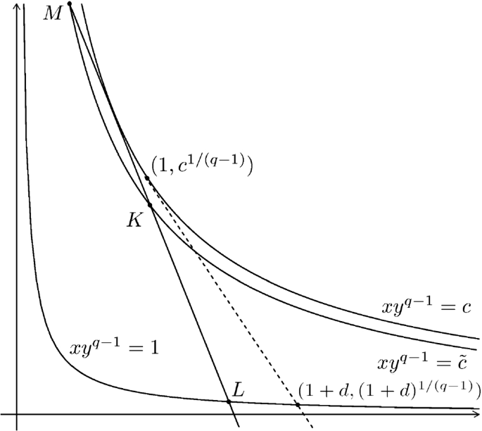

  

  The crucial three points $K=(1,\tilde{c}^{1/(q-1)})$, $L=\big (1+d(\tilde{c}),(1+d(\tilde{c}))^{1/(1-q)}\big )$ and $M=\big (1-\delta ,(\tilde{c}(1-\delta ))^{1/(1-q)}\big )$

  The points K, L, M are colinear: some simple algebra transforms this into the equality

  $$\begin{aligned} (\tilde{c}(1+d(\tilde{c})))^{1/(q-1)}\big (d(\tilde{c})+\delta -d(\tilde{c})(1-\delta )^{1/(1-q)}\big )=\delta , \end{aligned}$$

  (14)

  which will be useful later.

• Step 2. Construction. Now, recall the following simple measure-theoretic fact, which can be found in [7].

  Lemma 3.1

  For every $Q \in \mathcal {T}$ and every $\beta \in (0,1)$ there is a subfamily $F(Q) \subset \mathcal {T}$ consisting of pairwise disjoint subsets of Q such that

  $$\begin{aligned} \mu \left( \bigcup _{R\in F(Q)} R\right) =\sum _{R\in F(Q)} \mu (R)=\beta \mu (Q). \end{aligned}$$

  We use this fact recursively and construct an appropriate sequence $A_0\supset A_1\supset A_2\supset \ldots$ of subsets of X. The starting point is the choice $A_0=X$. To describe the inductive step, assume we have constructed $A_n$, which is a union of pairwise almost disjoint elements of $\mathcal {T}$, called the atoms of $A_n$. Of course, this condition is satisfied for $n=0$: we have $A_0=X\in \mathcal {T}$. Then, for each atom Q of $A_n$, we apply the above lemma with $\beta =d(\tilde{c})/(d(\tilde{c})+\delta )$ and get the corresponding subfamily F(Q). Put $A_{n+1}=\bigcup _Q\bigcup _{Q'\in F(Q)}Q'$, the first union taken over all atoms Q of $A_n$. Directly from the definition, this set is a union of the family $\{F(Q):Q \text{ an } \text{ atom } \text{ of } A_n\}$, which consists of pairwise disjoint elements of $\mathcal {T}$. We call these elements the atoms of $A_{n+1}$ and conclude the description of the induction step.

  As an immediate consequence of the above construction, we see that if Q is an atom of $A_k$, then for any $n\ge k$ we have

  $$\begin{aligned} \mu (Q\cap A_n)=\mu (Q)\left( \frac{d(\tilde{c})}{d(\tilde{c})+\delta }\right) ^{n-k} \end{aligned}$$

  and hence

  $$\begin{aligned} \mu (Q\cap (A_n\setminus A_{n+1}))=\mu (Q)\left( \frac{d(\tilde{c})}{d(\tilde{c})+\delta }\right) ^{n-k}\frac{\delta }{d(\tilde{c})+\delta }. \end{aligned}$$

  (15)

  Now, introduce the weights $w_1,\,w_2,\,\ldots ,\,w_m$ on X by the formula

  $$\begin{aligned} w_1^{p/p_1}=\sum _{n=0}^\infty \chi _{A_n\setminus A_{n+1}}(1-\delta )^n \end{aligned}$$

  and $w_2=w_3=\ldots =w_m\equiv 1$. Furthermore, for $j=1,\,2,\,\ldots ,\,m$, we let

  $$\begin{aligned} f_j=\sum _{n=0}^\infty \chi _{A_n\setminus A_{n+1}}(1+a_j\delta )^n, \end{aligned}$$

  where $a_1=(p_1d(\tilde{c}))^{-1}+p^{-1}-\varepsilon /p_1$ and, for $j\ge 2$, $a_j=(p_jd(\tilde{c}))^{-1}-\varepsilon /p_j$. Here $\varepsilon$ is a fixed positive parameter (which will be sent to zero at the end of the proof).

• Step 3. We have $[w]_{A_{\vec {P}}}\le c$. The equality $w_2=w_3=\ldots =w_m=1$ implies that $v_{\vec {w}}=w_1^{p/p_1}$ and $v_{\vec {w}}^{-p_1'/p}=w_1^{1-p_1'}$. Hence $[w]_{A_{\vec {P}}}\le c$ is equivalent to showing that $v_{\vec {w}}\in A_{q}$. This in turn amounts to saying that for any $Q\in \mathcal {T}$,

  $$\begin{aligned} \langle v_{\vec {w}}\rangle _Q \big \langle v_{\vec {w}}^{1/(1-q)}\big \rangle _Q^{q-1}\le c. \end{aligned}$$

  To prove this, we use (15) to obtain that for each atom Q of $A_k$ we have

  $$\begin{aligned} \langle v_{\vec {w}}\rangle _Q=\sum _{n=k}^\infty \left( \frac{d(\tilde{c})}{d(\tilde{c})+\delta }\right) ^{n-k}(1-\delta )^n\cdot \frac{\delta }{d(\tilde{c})+\delta }=\frac{(1-\delta )^k}{1+d(\tilde{c})} \end{aligned}$$

  (16)

  and

  $$\begin{aligned} \big \langle v_{\vec {w}}^{1/(1-q)}\big \rangle _Q&=\sum _{n=k}^\infty \left( \frac{d(\tilde{c})}{d(\tilde{c})+\delta }\right) ^{n-k}(1-\delta )^{n/(1-q)}\cdot \frac{\delta }{d(\tilde{c})+\delta }\\&=\frac{\delta }{d(\tilde{c})+\delta }(1-\delta )^{k/(1-q)}\cdot \left( 1-\frac{d(\tilde{c})}{d(\tilde{c})+\delta }(1-\delta )^{1/(1-q)}\right) ^{-1}\\&=\frac{c^{1/(q-1)}(1-\delta )^{k/(1-q)}}{(1+d(\tilde{c}))^{1/(1-q)}}, \end{aligned}$$

  where in the last line we have used (14). Suppose that R is an arbitrary element of $\mathcal {T}$. Then there is an integer k such that $R\subseteq A_{k-1}$ and $R\not \subseteq A_k$. We have

  $$\begin{aligned} \langle v_{\vec {w}}\rangle _R&=\frac{1}{\mu (R)}\int _{R\setminus A_k}v_{\vec {w}}\text{ d }\mu +\frac{1}{\mu (R)}\int _{R\cap A_k}v_{\vec {w}}\text{ d }\mu \\&=\frac{1}{\mu (R)}\int _{R\setminus A_k}(1-\delta )^{k-1}\text{ d }\mu +\frac{1}{\mu (R)}\int _{R\cap A_k}v_{\vec {w}}\text{ d }\mu . \end{aligned}$$

  By (16), applied to each atom Q of $A_k$ contained in R, we get

  $$\begin{aligned} int_{R\cap A_k}v_{\vec {w}}\text{ d }\mu =\frac{\mu (R\cap A_k)(1-\delta )^k}{1+d(\tilde{c})} \end{aligned}$$

  and hence, setting $\eta :=\mu (R\cap A_k)/\mu (R)$, we rewrite the preceding equality as

  $$\begin{aligned} \langle v_{\vec {w}}\rangle _R=(1-\eta )(1-\delta )^{k-1}+\eta \cdot \frac{(1-\delta )^k}{1+d(\tilde{c})}. \end{aligned}$$

  Similarly, we obtain

  $$\begin{aligned}&\langle v_{\vec {w}}^{1/(1-q)}\rangle _R=(1-\eta )(1-\delta )^{(k-1)/(1-q)}+\eta \cdot \frac{c^{1/(q-1)}(1-\delta )^{k/(1-q)}}{(1+d(\tilde{c}))^{1/(1-q)}}, \end{aligned}$$

  which implies

  $$\begin{aligned}&\langle v_{\vec {w}}\rangle _R\langle v_{\vec {w}}^{1/(1-q)}\rangle _R^{q-1}\\&=\bigg (\eta (1-\delta )+(1-\eta )(1+d(\tilde{c}))\bigg )\bigg (\eta (1-\delta )^{\frac{1}{1-q}}+(1-\eta )(1+d(\tilde{c}))^{\frac{1}{1-q} }\bigg )^{q-1}. \end{aligned}$$

  This number does not exceed c. Indeed, the right-hand side can be rewritten as

  $$\begin{aligned} (\eta M_x+(1-\eta )L_x)(\eta M_y+(1-\eta )L_y)^{q-1}, \end{aligned}$$

  where $M_x,\,M_y$ and $L_x$, $L_y$ are the coordinates of the points M and L (see Fig. 2). As $\eta$ ranges from 0 to 1, the point $\eta M+(1-\eta )L$ runs over the line segment ML which is entirely contained in $\{(x,y):xy^{q-1}\le c\}$. Since R was arbitrary, we obtain the desired $A_{\vec {P}}$ condition: $[w]_{A_{\vec {P}}}\le c$.

• Step 4. Completion of the proof. In the same manner as above, one verifies that if Q is an atom of $A_k$, then

  $$\begin{aligned} \langle f_j\rangle _Q =\sum _{n\ge k}(1+a_j\delta )^n \left( \frac{d(\tilde{c})}{d(\tilde{c})+\delta }\right) ^{n-k}\frac{\delta }{d(\tilde{c})+\delta }=\frac{(1+a_j\delta )^k}{1-a_jd(\tilde{c})}. \end{aligned}$$

  Note that the ratio of the above geometric series, is equal to

  $$\begin{aligned} \frac{(1+a_j\delta )d(\tilde{c})}{d(\tilde{c})+\delta }=1+\frac{(a_j d(\tilde{c})-1)\delta }{d(\tilde{c})+\delta }<1+\frac{(p_j^{-1}-1)\delta }{d(\tilde{c})+\delta }<1, \end{aligned}$$

  so the series is convergent. Hence, on $A_k$ (and hence also on $A_k\setminus A_{k-1}$) we have

  $$\begin{aligned} \mathcal {M}\vec {f}\ge \prod _{j=1}^m \langle f_j\rangle _Q=\prod _{j=1}^m \frac{(1+a_j\delta )^k}{1-a_jd(\tilde{c})} \end{aligned}$$

  and therefore

  $$\begin{aligned} \Vert \mathcal {M}\vec {f}\Vert _{L^p(v_{\vec {w}})}&\ge \left( \sum _{n\ge 0}\left( \prod _{j=1}^m \frac{(1+a_j\delta )^{n}}{1-a_jd(\tilde{c})}\right) ^p (1-\delta )^n\left( \frac{d(\tilde{c})}{d(\tilde{c})+\delta }\right) ^n \frac{\delta }{d(\tilde{c})+\delta }\right) ^{1/p}. \end{aligned}$$

  The ratio of the geometric series in the parentheses is given by

  $$\begin{aligned} \prod _{j=1}^m (1+a_j\delta )^{p}(1-\delta )&\left( \frac{d(\tilde{c})}{d(\tilde{c})+\delta }\right) \\&=1+\left[ p(a_1+a_2+\ldots +a_m)-1-(d(\tilde{c}))^{-1} \right] \delta +o(\delta )\\&=1-\varepsilon \delta +o(\delta ) \end{aligned}$$

  as $\delta \rightarrow 0$. Thus the series is convergent and we obtain

  $$\begin{aligned} \Vert \mathcal {M}\vec {f}\Vert _{L^p(v_{\vec {w}})}&\ge (d(\tilde{c})\varepsilon )^{-1/p}\prod _{j=1}^m (1-a_jd(\tilde{c}))^{-1}+O(\delta ). \end{aligned}$$

  On the other hand, an analogous computation shows that

  $$\begin{aligned} \Vert f_1\Vert _{L^{p_1}(w_1)}&=\left( \sum _{n\ge 0} (1+a_1\delta )^{np_1}(1-\delta )^{np_1/p}\left( \frac{d(\tilde{c})}{d(\tilde{c})+\delta }\right) ^n \frac{\delta }{d(\tilde{c})+\delta }\right) ^{1/p_1}\\&=\left( p_1d(\tilde{c})\left( (p_1d(\tilde{c}))^{-1}+p^{-1}-a_1\right) \right) ^{-1/p_1}+O(\delta )=(d(\tilde{c})\varepsilon )^{-1/p_1}+O(\delta ) \end{aligned}$$

  and for $j\ge 2$,

  $$\begin{aligned} \Vert f_j\Vert _{L^{p_j}(w_j)}&=\left( \sum _{n\ge 0}(1+a_j\delta )^{np_j}\left( \frac{d(\tilde{c})}{d(\tilde{c})+\delta }\right) ^n \frac{\delta }{d(\tilde{c})+\delta }\right) ^{1/p_j}\\&=(1-a_jp_jd(\tilde{c}))^{-1/p_j}+O(\delta )=( d(\tilde{c})\varepsilon )^{-1/p_j}+O(\delta ). \end{aligned}$$

  Putting the above facts together (and noting that $d(\tilde{c})\rightarrow d(q,c)$ as $\delta \rightarrow 0$), we get

  $$\begin{aligned} \limsup _{\delta \rightarrow 0}\frac{\Vert \mathcal {M}\vec {f}\Vert _{L^p(v_{\vec {w}})}}{\prod _{j=1}^m \Vert f_j\Vert _{L^{p_j}(w_j)}}\ge \prod _{j=1}^m (1-a_jd(q,c))^{-1}. \end{aligned}$$

  Finally, we check that the constant on the right converges, as $\varepsilon \rightarrow 0$, to

  $$\begin{aligned} \left( 1-\frac{p_1'd(q,c)}{p}\right) ^{-1}\prod _{j=1}^m p_j'=(c(1+d(q,c)))^{p_1'/p}\prod _{j=1}^m p_j'. \end{aligned}$$

  This yields the desired lower bound for the optimal constant.

References

Buckley, S.M.: Estimates for operator norms on weighted spaces and reverse Jensen inequalities. Trans. Am. Math. Soc. 340, 253–272 (1993)
Chen, W., Damián, W.: Weighted estimates for the multisublinear maximal function. Rend. Circ. Mat. Palermo 62, 379–391 (2013)
Damián, W., Lerner, A.K., Pérez, C.: Sharp weighted bounds for multilinear maximal functions and Calderón–Zygmund operators. J. Fourier Anal. Appl. 21(1), 161–181 (2015)
Hytönen, T., Pérez, C.: Sharp weighted bounds involving \(A_\infty\). Anal. PDE 6, 777–818 (2013)
Lerner, A.K., Ombrosi, S., Pérez, C., Torres, R.H., Trujillo-González, R.: New maximal functions and multiple weights for the multilinear Calderón-Zygmund theory. Adv. Math. 220, 1222–1264 (2009)
Li, K., Moen, K., Sun, W.: The sharp weighted bound for multilinear maximal functions and Calderón–Zygmund operators. J. Fourier Anal. Appl. 20(4), 751–765 (2014)
Melas, A.D.: The Bellman functions of dyadic-like maximal operators and related inequalities. Adv. Math. 192, 310–340 (2005)
Muckenhoupt, B.: Weighted norm inequalities for the Hardy maximal function. Trans. Am. Math. Soc 165, 207–226 (1972)
Osękowski, A.: Best constants in Muckenhoupt’s inequality. Ann. Acad. Sci. Fenn. Math. 42, 889–904 (2017)
Acknowledgements
The author would like to thank an anonymous Referee for the careful reading of the paper and a few helpful suggestions. No funding was received to assist with the preparation of this manuscript.
Author information
Authors and Affiliations
Corresponding author
Additional information
Publisher's Note
Springer Nature remains neutral with regard to jurisdictional claims in published maps and institutional affiliations.
Rights and permissions
Open Access This article is licensed under a Creative Commons Attribution 4.0 International License, which permits use, sharing, adaptation, distribution and reproduction in any medium or format, as long as you give appropriate credit to the original author(s) and the source, provide a link to the Creative Commons licence, and indicate if changes were made. The images or other third party material in this article are included in the article's Creative Commons licence, unless indicated otherwise in a credit line to the material. If material is not included in the article's Creative Commons licence and your intended use is not permitted by statutory regulation or exceeds the permitted use, you will need to obtain permission directly from the copyright holder. To view a copy of this licence, visit http://creativecommons.org/licenses/by/4.0/.
About this article
Cite this article
Osękowski, A. Weighted estimates for the multilinear maximal operator. Collect. Math. 75, 379–394 (2024). https://doi.org/10.1007/s13348-022-00390-5
Received:
Accepted:
Published:
Issue Date:
DOI: https://doi.org/10.1007/s13348-022-00390-5