


1. Introduction
The estimation of mean and covariance functions plays a fundamental role in the analysis of functional data. How to appropriately model these functions is fascinating but challenging and has drawn much attention from statisticians in the past several decades. Influential works in this area include, but are not limited to, Rice and Silverman [Reference Rice and Silverman19], James et al. [Reference James, Hastie and Sugar9], Yao et al. [Reference Yao, Müller and Wang23], Li and Hsing [Reference Li and Hsing12], Peng and Paul [Reference Peng and Paul17], Cai and Yuan [Reference Cai and Yuan2], Ogden and Greene [Reference Ogden and Greene16], Chen and Müller [Reference Chen and Müller4], Xiao et al. [Reference Xiao, Li and Ruppert22], Zhou et al. [Reference Zhou, Lin and Liang26], Meister [Reference Meister15] and the references therein. Well-known monographs by Ramsay and Silverman [Reference Ramsay and Silverman18], Ferraty and Vieu [Reference Ferraty and Vieu7] and Kokoszka and Reimherr [Reference Kokoszka and Reimherr11] provided comprehensive discussions on the methods and applications.
Nowadays, an important question is how to estimate mean and covariance function with available covariate information. Such covariate information is commonly encountered in biomedical studies and informational sciences, which requires us to use the additional covariates to model the trajectory realistically. They have been receiving increasing attention recently [Reference Cardot and Sarda3,Reference Stallrich, Islam, Staicu, Crouch, Pan and Huang20,Reference Wu, Fan and Müller21]. Specifically, Chiou and Wang [Reference Chiou, Müller and Wang6] discussed the influence of covariates on a sample of response curves through a semiparametric model under the framework of dense functional data. Jiang and Wang [Reference Jiang and Wang10] described a general approach incorporating a covariate effect to model the mean and covariance function for sparse longitudinal data. Liebl [Reference Liebl14] considered inference problem for the mean and covariance functions of covariate adjusted functional data. Zhang et al. [Reference Zhang, Lin, Liu, Liu and Li25] proposed a new functional regression model with covariate-dependent mean and covariance structures to analyze the Avon Longitudinal Study of Parents and Children datasets.
However, the aforementioned works only address the sparse or dense functional data. Little is known on how to incorporate covariate information in modeling for a general type of functional data, so our goal in this paper is to provide a general weighing approach to incorporate the covariate information that is applicable to both dense and sparse functional data. For the sake of simplicity and convenience, throughout this article, we consider the case of a one-dimensional covariate  $Z_{i}$ for
  $i=1,\ldots,n$. Let
  $Y_{ij}$ be the
  $j$th observation of the random function
  $X_i(T_{ij},Z_i)$, made at a discrete time points
  $T_{ij}\in [0,1]$ with a covariate
  $Z_{i}\in [0,1]$ and independent identically distributed measurement errors
  $\varepsilon _{ij}$ for
  $j=1,\ldots, m_i$. Thus, the observed data are often written as
 \begin{equation} Y_{ij}=X_{i}(T_{ij},Z_i)+\varepsilon_{ij}\quad {\rm for}\ i=1,\ldots,n, \end{equation}
where the sampling locations  $T_{ij}$ and
  $Z_{i}$ are independently drawn from a distribution of random variables
  $T$ and
  $Z$ with density function
  $f(\cdot )$ and
  $g(\cdot )$ on bounded support
  $[0,1]$, respectively. One is generally interested in estimating mean function
  $E\{X_{i}(t,z)\}=\mu (t,z)$ and covariance function
  ${\rm cov}\{X_{i}(t,z),X_{i}(s,z)\}=K(t,s,z)$ based on the observation of
  $Y_{ij}$ for
  $j=1,\ldots, m_i,i=1,\ldots,n$.
To broaden the applicability of the aforementioned model, we propose to estimate the mean and covariance functions not only by allowing the functions to depend on the additional scalar covariate but also in the framework of the general weighted local linear smoothing. We further carefully demonstrate the uniform convergence rate for the proposed estimators. The derived convergence rates of mean and covariance functions provide an essential theoretical result for the future research, such as functional principal component analysis and functional regression issues.
The rest of the article is organized as follows. We would introduce the proposed estimation procedure in Section 2.1 and present theoretical results in Section 2.2. Regularity conditions and technical proofs are delegated to the Appendix. Simulation studies are conducted to verify the theoretical results. The approach is applied to analyze the growth curves of children dataset and produce meaningful and interesting results. Both are shown in Section 3. The concluding remarks are given in Section 4.
2. Methodology
2.1. Estimation procedure
This section describes the method of estimation of mean and covariance functions. To obtain mean function  $\mu (t,z)$ and covariance function
  $K(s,t,z)$, we apply the weighted local linear smoothing method [Reference Zhang and Wang24]. Specifically, the weight
  $\omega _i$ is attached to each observation for the
  $i$th subject such that
  $\sum _{i=1}^n m_i\omega _i=1$, we define the weighted local linear smoother for
  $\mu (t,z)$ by minimizing
 \begin{align} \widehat{\boldsymbol\beta}& = \arg\min_{\boldsymbol{\beta}}\sum_{i=1}^n\omega_{i}\sum_{j=1}^{m_i} K_{h_{\mu t}}({T_{ij}-t})K_{h_{\mu z}}({Z_{i}-z}) \nonumber\\ & \quad \times \{Y_{ij} -\beta_0 -\beta_1(T_{ij}-t) -\beta_2(Z_i-z) \}^2, \end{align}
with respect to  $\boldsymbol {\beta }=(\beta _0,\beta _1,\beta _2) ^{\rm T}$. The estimate of
  $\mu (t,z)$ is then
  $\widehat \mu (t,z)=\widehat \beta _0$. Once the
  $\widehat \mu (\cdot,\cdot )$ is obtained, we are then ready to estimate the covariance function
  $G(t,s,z)$. Let
  $G_{ijk}=\{Y_{ij}-\widehat \mu (T_{ij},Z_i)\} \{Y_{ik}-\widehat \mu (T_{ik},Z_i)\}$ be the input data, and the weight
  $\nu _i$ is attached to each
  $G_{ijk}$ for the
  $i$th subject such that
  $\sum _{i=1}^n m_i(m_i-1)\nu _i=1$. The weighted local linear smoother for the covariance function
  $G(t,s,z)$ is
  $\widehat G(t,s,z) =\widehat \beta _0$ where
  $\boldsymbol {\beta }=(\beta _0,\beta _1,\beta _2,\beta _3) ^{\rm T}$,
 \begin{align} \widehat{\boldsymbol\beta} & =\arg\min_{\boldsymbol{\beta}} \sum_{i=1}^n \nu_{i}\sum_{1\leq j\neq k\leq m_i} K_{{h_{G t}}}({T_{ij}-t})K_{{h_{G t}}}({T_{ik}-s}) K_{{h_{G z}}}({Z_{i}-z}) \nonumber\\ & \quad \times \{ G_{ijk} -\beta_0 -\beta_1(T_{ij}-t) -\beta_2(T_{ik}-s) +\beta_3(Z_{i}-z) \}^2. \end{align}
The bandwidths  $h_{\mu t}$ and
  $h_{\mu z}$ for the estimated mean function are chosen via the leave-one-curve-out cross validation and the bandwidths
  $h_{G t}$ and
  $h_{G z}$ of the covariance function estimators are chosen via a
  $10$-fold cross-validation procedure to save computing time throughout this article. More details about choices of
  $\omega _i$ and
  $\nu _i$ of (2) and (3) can be found in Huang et al. [Reference Huang, Wu and Zhou8] and Zhang and Wang [Reference Zhang and Wang24]. In general, when the observation is sparse, assignment
  $\omega _{i}=1/\sum _{i=1}^{n}m_{i}$ along with
  $\nu _{i}=1/\sum _{i=1}^{n}m_{i}(m_{i}-1)$ leads to the same weight to each observation scheme (OBS); often in the dense observation, assignment
  $\omega _{i}=1/(nm_{i})$ along with
  $\nu _{i}=1/nm_{i}(m_{i}-1)$ leads to the same weight to each subject scheme (SUBJ). Although OBS and SUBJ are the most commonly used schemes, for some cases, Zhang and Wang [Reference Zhang and Wang24] suggested using a mixture of the OBS and SUBJ schemes (MIX). That is,
  $\omega _i=\alpha _1/(\sum _{i=1}^n m_i)+(1-\alpha _1)/(nm_i)$ and
  $\nu _i=\alpha _2/\{\sum _{i=1}^n m_i(m_i-1)\}+(1-\alpha _2)/\{nm_i(m_i-1)\}$ for some
  $0\le \alpha _1,\alpha _2\le 1$. Moreover, they showed that the MIX scheme was likely to achieve a better performance. In our simulation part, we will see that this weighing scheme is also likely to be better than OBS and SUBJ with incorporating covariate information.
2.2. Asymptotic results
In this section, we establish the uniform convergence rates for the estimates. Our results cover the case of sparse designs, where the number of design points  $m_i$ is bounded, and the case of dense designs, where
  $m_i\rightarrow \infty$. The additional assumptions and proof of these results are relegated to Appendix. Based on the general weighing scheme, we provide the uniform convergence rates of mean and covariance function estimators in Theorems 1 and 2, respectively.
Theorem 1. Under conditions (A1)–(A5) and (B1)–(B4) in the Appendix,
 $$\sup_{t,z\in[0,1]}|\widehat\mu(t,z)-\mu(t,z)| = O(h_{\mu t}^2+h_{\mu z}^2+h_{\mu t}h_{\mu z}+\delta_{n1})\quad \text{a.s.},$$
where
 $$\delta_{n1}= \left[ \log (n) \left\{ \frac{\sum_{i=1}^n m_{i}\omega_i^2}{h_{\mu t}h_{\mu z}} +\frac{\sum_{i=1}^n m_{i}(m_i-1)\omega_i^2}{h_{\mu z}} \right\} \right]^{1/2}.$$
Theorem 2. Under conditions (A1)–(A6) and (C1)–(C4) in the Appendix,
 \begin{align*} & \sup_{s,t,z\in[0,1]} |\widehat G(t,s,z)-G(t,s,z)|\\ & \quad = O( h_{\mu t}^2+h_{\mu z}^2+h_{\mu t}h_{\mu z}+\delta_{n1} +h_{Gt}^2+h_{Gz}^2+h_{Gt}h_{Gz}+\delta_{n2}) \quad \text{a.s.}, \end{align*}
where
 \begin{align*} \delta_{n2}& =\left[ \log (n) \left\{ \frac{\sum_{i=1}^n m_i(m_i-1)\nu_i^2}{h_{Gt}^2h_{Gz}} +\frac{\sum_{i=1}^n m_i(m_i-1)(m_i-2)\nu_i^2}{h_{Gt}h_{Gz}} \right.\right.\\ & \quad \left.\left. +\frac{\sum_{i=1}^n m_i(m_i-1)(m_i-2)(m_i-3)\nu_i^2}{h_{Gz}} \right\} \right]^{1/2}. \end{align*}
The results in Theorems 1 and 2 are natural extensions of Theorems 5.1 and 5.2 of Zhang and Wang [Reference Zhang and Wang24] for the case of additional covariate information available, respectively. Similar conclusion for the OBS scheme was established by Chen and Müller [Reference Chen and Müller4].
3. Numerical studies
3.1. Simulation results
To assess which weighing scheme is better in the case where covariate information is incorporated, we evaluate the finite-sample numerical performances of the most commonly used OBS and SUBJ schemes, together with the weighing schemes based on their mixture as defined in Section 2. The simulation is set as follows: for each subject  $i$, the covariate-adjusted true trajectories are generated as
  $Y_i(t)=\mu (t,z)+\sum _{k=1}^2\xi _{ik}\psi _{k}(t,z)+\epsilon _i(t)$, where the covariate
  $z$ is generated from
  $U(0,1)$, and mean function is
  $\mu (t,z)=(1+z)(t+\sin (t))$. The principal component scores are
  $\xi _{ik}\sim \mathcal {N}\{0,\lambda _k(z)\}$ for
  $k=1,2$ and the eigenfunctions are
  $\psi _{1}(t,z)=\sqrt {2}\sin (\pi (t+z/2))$ and
  $\psi _{2}(t,z)=-\sqrt {2}\cos (\pi (t+z/2))$, respectively. We set
  $\{\lambda _{1}(z),\lambda _{2}(z)\}=(z/9,z/36)$ and
  $\epsilon _{i}(t)\sim \mathcal {N}(0,0.2)$.
For more generality in practice, we provide the simulation studies under different number of observation points setting, which include sparse, dense and mixture of them shown as follows:
Case 1:
 $m_i$ is sampled with equal probability from $\{2,\ldots,6\}$.
Case 2:
$m_i$ is sampled from a discrete uniform distribution on the interval $[n/6,n/3]$.Case 3:
$m_i=n/4$ with probability $1/2$, and follows Case 1 with probability $1/2$.


We compare the performance of three different weighing scheme using the corresponding mean integrated square errors (MISE) for the  $\widehat \mu$ defined as below
 $$\mathrm{MISE} (\widehat\mu, h_\mu) =\frac{1}{n}\sum_{i=1}^n \int \{\widehat\mu(t, z_{i})-\mu(t, z_{i})\}^2 \,d t.$$
To evaluate the covariance estimators, we assume that the mean function  $\mu$ is known so that the covariance estimation is disentangled from the mean estimation and define the MISE of
  $\widehat G$ as follows:
 $$\operatorname{MISE} (\widehat G, h_G)=\frac{1}{n}\sum_{i=1}^n \iint \{\widehat G(s, t,z_i)-G(s, t,z_i)\}^2\, d s \,d t.$$
In each case, the sample size is 50, 100 and 200, respectively. We present the mean and standard deviation (in parentheses) of the MISE over 200 repetitions for each case. Hereafter, estimators with the subscript “obs,” “subj” and “mix” represent the OBS, SUBJ and MIX estimators, respectively.
In Table 1, similar to the case where covariate information is not incorporated, the OBS scheme outperforms the SUBJ scheme in Case 1 and Case 3, while the SUBJ scheme is superior in Case 2. Moreover, as expected, the performance improves as the number of subjects increases. With respect to MISE of covariance function from Table 2, we have similar results to their counterparts in Table 1, which conforms with the case of ignoring the covariate information.
Table 1. MISE of the estimator of mean function, where  $\widehat \mu _{\mathrm {obs}}$ is the OBS scheme,
  $\widehat \mu _{\mathrm {subj}}$ refers to SUBJ scheme,
  $\widehat \mu _{\mathrm {mix}}$ denotes the mixture of the above two weighing scheme (
 $\alpha _1=1/2$).

The corresponding standard errors are in parentheses.
Table 2. MISE of the estimator of covariance function, where  $\widehat G_{\mathrm {obs}}$ is the OBS scheme,
  $\widehat G_{\mathrm {subj}}$ refers to SUBJ scheme,
  $\widehat G_{\mathrm {mix}}$ denotes the mixture of the above two weighing scheme (
 $\alpha _2=1/2$).
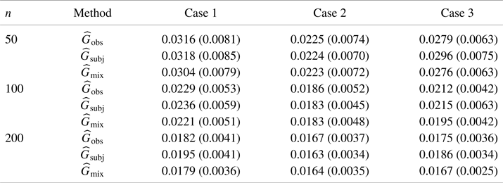
The corresponding standard errors are in parentheses.
As shown in Tables 1 and 2, both  $\widehat \mu _{\mathrm {mix}}$ and
  $\widehat G_{\mathrm {mix}}$ performed equally well or better than the counterparts of OBS and SUBJ estimators. This provides the numerical evidence for the benefit of using a mixture of the OBS and SUBJ schemes as discussed in Section 2.
3.2. Application to children growth data
We apply the proposed methodology to analyze a real medical study dataset about the growth curves of children, which is publicly available on https://content.sph.harvard.edu/fitzmaur/ala/fev1.txt. This dataset was presented by Brunekreef et al. [Reference Brunekreef, Janssen, de Hartog, Harssema, Knape and van Vliet1] and was commonly used as an example for a longitudinal study designed to characterize lung growth as measured by changes in pulmonary function in children and adolescents.
The dataset consists of 300 children, with a minimum of 1 and a maximum of 12 observations over time. The following four variables are included: age (ranging from 6 to 18 years old), height,  ${\rm FEV}_1$ (forced expiratory volume in one second) and initial height, which is obtained from a randomly selected subset of the participants living in Topeka, Kansas in USA. What we are interested in is to explore the influence of children's initial height on the shape changes of the mean functions of height's curve. Therefore, the adjusted covariate is initial height and we exclude the children whose observations are less than two times, such that the sample size
  $n=258$. Since the range of children's age is sparse (the maximum is 12 observations), we adopt OBS weighing scheme to model the height curve.
To compare the developed approach with the approach that does not incorporate the initial height information, we also display the fitted curves by using the conventional OBS weighing scheme estimation procedure [Reference Zhang and Wang24]. We randomly select four estimated mean height curves shown in Figure 1. The overall trend of the height curve as shown is incremental with a decreasing rate of growth, which is consistent with common knowledge. Specifically, the left top plot shows that our estimation procedure is closer to the observed height's curve compared with the approach without the initial height adjusted. According to other plots, we have similar results. This demonstrates that the data support the simple covariate-adjusted approach when modeling curves. The differences between the two estimated methods may somewhat claim that the proposed method is more efficient numerically than conventional approaches without incorporating covariate information. Such an extension in this paper could be valuable for doctors who study how the children's height changes with their age when covariate information is available.

Figure 1. Plots of an estimated mean function of children's height. The black dashed lines are the observed height's curve. The blue solid lines are the estimated mean function of height by Zhang and Wang [Reference Zhang and Wang24] and the red solid lines denote the curve estimated by our estimation procedure.
3.3. Application to diffusion tensor imaging study
The proposed method is also applied to a real data set of diffusion tensor imaging (DTI). In diffusion data analysis, fractional anisotropy (FA), which quantifies the directional strength of white matter tract structure, at a particular location, is one of the most used measures and has been widely applied to statistical analyses in many imaging studies, see, such as Zhu et al. [Reference Zhu, Li and Kong27], Li et al. [Reference Li, Huang, Hongtu and Initiative13] and reference therein. The data can be downloaded from the ADNI publicly available database (https://adni.loni.usc.edu/) or http://www.nitrc.org/projects/fadtts/.
We are interested in delineating the trend of the variability of these functional FA with a set of available covariates of interest, such as age. In particular, we use  $64$ healthy infants from the neonatal project on early brain development. The gestational ages of these infants range from
  $262$ to
  $433$ days, and their mean gestational age is
  $298$ days with standard deviation
  $17.6$ days. The dataset was preprocessed by Zhu et al. [Reference Zhu, Li and Kong27]. Finally, we fit model (1) to the FA values from
  $64$ subjects at
  $75$ grid points along the genu tract of the corpus callosum, in which
  $Z_i=\text {Age}$. Since the data are dense, SUBJ is adopted.
Figure 2 presents the three randomly selected estimated FA trajectories with age information adjusted, as well as the traditional non-information adjusted estimation curves. It also shows that the proposed method is more efficient. Moreover, the results confirm that neonatal microstructural development of FA correlates with age. Such findings are consistent with those of previous works. This shows that the proposed estimate is more reasonable in describing the true characteristic of the mean function.

Figure 2. Plots of the estimated mean function of functional FA. The black dashed lines are the observed FA values. The blue solid lines are the estimated mean function of FA without age adjusted and the red solid lines denote the trajectory estimated by our estimation procedure.
4. Discussion
In this paper, we focused on covariate adjusted local linear smoothers when estimating the mean and covariance functions. This is an important extension for the study of functional mean-covariance model, because we incorporate the available covariate information that may improve the accuracy of estimation. Moreover, we are particularly interested in the framework of general weighing scheme which incorporates the commonly used OBS and SUBJ schemes. The carefully derived convergence rates in the framework of general weighing scheme expanded the results that ignore the covariate information. Numerical performances of OBS and SUBJ schemes are also systematically compared.
It is also of great interest to establish the asymptotic distribution and optimal convergence rate of  $\widehat \mu (t,z)$ and
  $\widehat G(t,z)$ under the general weighing framework, which we left for future work. Furthermore, the general weighing framework may be used in functional data regression, classification, clustering, etc., and hence the theoretical results here could be extended to those cases as well. This will also be pursued in future work.
Acknowledgments
We thank two reviewers, an associate editor and the editor, for their most helpful comments that lead to substantial improvements in the paper. The work is supported by National Natural Science Foundation of China (project number: 12101270, 11871252, 11971034). Data used in the preparation of this article were obtained from the Alzheimer's Disease Neuroimaging Initiative (ADNI) database (adni.loni.usc.edu). As such, the investigators within the ADNI contributed to the design and implementation of ADNI and/or provided data but did not participate in the analysis or writing of this report. A complete listing of ADNI investigators can be found at: http://adni.loni.usc.edu/wpcontent/uploads/how_to_apply/ADNI_Acknowledgement_List.pdf.
Conflict of interest
The authors have not disclosed any competing interests.
Appendix
A.1. Conditions
Similar to the conditions in Chen and Müller [Reference Chen and Müller4], Chen et al. [Reference Chen, Delicado and Müller5] and Zhang and Wang [Reference Zhang and Wang24], the following conditions are imposed to facilitate the proofs.
Conditions for kernel function and time points
(A1)
$K(\cdot )$ is a symmetric probability density function on $[-1,1]$ and
$$\sigma_{K}^{2}=\int u^{2}K(u)\,du \lt \infty,\quad \|K\|^{2}=\int K(u)^{2}\,du \lt \infty$$
(A2)
$K(\cdot )$ is Lipschitz continuous and there exists $0 \lt L \lt \infty$ such that
This implies$$|K(u)-K(v)|\leq L|u-v|,\quad {\rm for\ any}\ u,v\in[0,1].$$
$K(\cdot )\leq M_{K}$ for a constant $M_{K}$.(A3)
$\{T_{ij}:i=1,\ldots,n,j=1,\ldots,m_i\}$, are i.i.d. copies of a random variable $T$ defined on [0,1]. The density $f(\cdot )$ of $T$ is bounded from below and above: $0 \lt m_{f}\leq \min _{t\in [0,1]} f(t)\leq \max _{t\in [0,1]} f(t)\leq M_{f} \lt \infty$.(A4)
$f^{(2)}(\cdot )$ and $g^{(2)}(\cdot )$, the second derivatives of $f(\cdot )$ and $g(\cdot )$, are bounded, respectively.(A5)
$\partial ^2\mu (t,z)/\partial t$ and $\partial ^2\mu (t,z)/\partial z$, the second derivatives of ${\mu }(t,z)$ with respect to $t$ and $z$, are bounded on $[0,1]^{2}$, respectively.(A6)
$\partial ^{2} G(s,t,z)/\partial s^{2}$, $\partial ^{2} G(s,t,z)/\partial t^{2}$, $\partial ^{2} G(s,t,z)/\partial z^{2}$, $\partial ^{2} G(s,t,z)/\partial s\partial t$, $\partial ^{2} G(s,t,z)/\partial s\partial z$, and $\partial ^{2} G(s,t,z)/\partial t\partial z$ are bounded on $[0,1]^{3}$.


Conditions for mean function estimation
(B1)
$h_{\mu t}\rightarrow 0$. For some finite $\rho _{\mu }$, ${h_{\mu t}}/{h_{\mu z}}\rightarrow \rho _{\mu }$.(B2)
$\log (n){\sum _{i=1}^n m_{i}\omega _i^2}/{h_{\mu t}h_{\mu z}}\rightarrow 0$, and $\log (n){\sum _{i=1}^n m_{i}(m_i-1)\omega _i^2}/{h_{\mu z}}\rightarrow 0$.(B3) For some
$\alpha \gt 2$, $E\{\sup _{t,z\in [0,1]} |U(t,z)|^{\alpha }\} \lt \infty$, $E|\varepsilon |^{\alpha } \lt \infty$ and
$$n\left\{\sum_{i=1}^n m_i\omega_i^2 h_{\mu t}h_{\mu z} +\sum_{i=1}^n m_i(m_i-1)\omega_i^2 h_{\mu t}^2 h_{\mu z} \right\}\left\{\frac{\log(n)}{n}\right\}^{2/\alpha-1} \rightarrow\infty.$$
(B4)
$\sup _n (n\max _{i}m_i\omega _{i})\leq B \lt \infty$.


Conditions for covariance function estimation
(C1)
$h_{Gt}\rightarrow 0$ and ${h_{Gt}}/{h_{Gz}}\rightarrow \rho _G$ for some $0 \lt \rho _G \lt \infty$.(C2)
$\log (n){\sum _{i=1}^n m_i(m_i-1)\nu _i^2}/{h_{Gt}^2h_{Gz}}\rightarrow 0$, $\log (n){\sum _{i=1}^n m_i(m_i-1)(m_i-2)\nu _i^2}/{h_{Gt}h_{Gz}}\rightarrow 0$, $\log (n){\sum _{i=1}^n m_i(m_i-1)(m_i-2)(m_i-3)\nu _i^2}/{h_{Gz}}\rightarrow 0$.(C3) For some
$\beta \gt 2$, $E\{\sup _{t,z\in [0,1]}|U(t,z)|^{2\beta }\} \lt \infty$, $E|\varepsilon |^{2\beta } \lt \infty$, and
\begin{align*} & n \left\{ \sum_{i=1}^n m_i(m_i-1)\nu_i^2 h_{Gt}^2 h_{Gz} +\sum_{i=1}^n m_i(m_i-1)(m_i-2)\nu_i^2 h_{Gt}^3 h_{Gz} \right.\\ & \quad \left.+\sum_{i=1}^n m_i(m_i-1)(m_i-2)(m_i-3)\nu_i^2 h_{Gt}^4 h_{Gz} \right\} \left\{\frac{\log(n)}{n}\right\}^{2/\beta-1} \rightarrow \infty. \end{align*}
(C4)
$\sup _n(n\max _i m_i(m_i-1)\nu _{i})\leq B^\prime \lt \infty$.


Conditions (A1)–(A6) are standard in the literature of functional data analysis (FDA) and nonparametric smoothing such as Yao et al. [Reference Yao, Müller and Wang23]. Conditions (B1)–(B4) are used to guarantee the consistency of the estimator of the mean function. Their counterparts for the OBS and SUBJ schemes are commonly used in FDA, similar versions can refer to Chen and Müller [Reference Chen and Müller4]. Likewise, the Conditions (C1)–(C4) are used to establish the consistency of the estimated covariance function. Condition (C1) is a mild condition that requires the bandwidth  $h_{Gt}$ and
  $h_{Gz}$ to converge to zero at the same rate. Conditions (C2) and (C3) impose restrictions on
  $m_i$,
  $n$ and
  $h_{Gt} (h_{Gz})$ in theory. Condition (C4) allows
  $m_i$ is different for each subject
  $i$ but not too irregular. More detailed demonstration can refer to Zhang and Wang [Reference Zhang and Wang24].
A.2. Auxiliary results and proofs
In this subsection, we provide detailed proofs for the estimators in this paper. Below, for any square matrix  ${\mathbf {A}}$,
  $|{\mathbf {A}}|$ denotes the determinant. We denote
 $$L(t,z)=\sum_{i=1}^n \omega_i\sum_{j=1}^{m_i} K\left(\frac{T_{ij}-t}{h_{\mu t}}\right) K\left(\frac{Z_i-z}{h_{\mu z}}\right)U_{ij}^+,$$
where  $U_{ij}^+$ is the positive part of
  $U_{ij}$ and
  $U_{ij}:=U(T_{ij},Z_{i})=Y_{ij}-\mu (T_{ij},Z_i)$.
The following lemma is used to prove Theorem 1.
Lemma A.1. Under the assumptions for Theorem 1,
 $$\sup_{t,z\in[0,1]}|L(t,z)-EL(t,z)|=O(a_n) \quad \text{a.s.},$$
where
 $$a_n = \left[ \log (n) \left\{ \sum_{i=1}^n m_i\omega_i^2 h_{\mu t}h_{\mu z} +\sum_{i=1}^n m_i(m_i-1)\omega_i^2 h_{\mu t}^2 h_{\mu z} \right\} \right]^{1/2}.$$
Proof. For the sake of simplicity, we denote  $A_{n}=a_n\{n/\log (n)\}$. By (B2), we can choose
  $\rho$ such that
  $n^\rho h_{\mu t}a_n\rightarrow \infty$ (i.e.,
  $n^\rho h_{\mu z}a_n\rightarrow \infty$ by (B1)) and let
  $\chi (\rho )$ be an equally sized mesh on
  $[0,1]^{2}$ with grid
  $n^{-\rho }$ by
  $n^{-\rho }$. Observe that
 \begin{align*} \sup_{t,z\in[0,1]}|L(t,z)-EL(t,z)| & \le \sup_{t,z\in\chi(\rho)} \sup_{\substack{t,s,z,z^{\prime}\in[0,1]\\ |t-s|,|z-z^{\prime}|\leq n^{-\rho}}} |L(t,z)-L(s,z^{\prime})| \\ & \quad +\sup_{t,z\in\chi(\rho)} |L(t,z)-EL(t,z)| \\ & \quad +\sup_{t,z\in\chi(\rho)} \sup_{\substack{t,s,z,z^{\prime}\in[0,1]\\ |t-s|,|z-z^{\prime}|\leq n^{-\rho}}} |EL(t,z)-EL(s,z^{\prime})| \\ & \equiv Q_1+Q_2+Q_3. \end{align*}
We first consider  $Q_1$ and
  $Q_3$. For all
  $t$ and
  $z$, by (A2) and Hölder inequality, it follows that
 \begin{align*} Q_1& =\sup_{|t-s|,|z-z^{\prime}|\leq n^{-\rho}} |L(t,z)-L(s,z^{\prime})|\\ & \leq \sup_{|t-s|,|z-z^{\prime}|\leq n^{-\rho}} \left| \sum_{i=1}^n\omega_i\sum_{j=1}^{m_i}U_{ij}^+ K\left(\frac{Z_{i}-z}{h_{\mu z}}\right) \left\{K\left(\frac{T_{ij}-t}{h_{\mu t}}\right) -K\left(\frac{T_{ij}-s}{h_{\mu t}}\right)\right\}\right| \\ & \quad +\sup_{|t-s|,|z-z^{\prime}|\leq n^{-\rho}} \left| \sum_{i=1}^n \omega_i \sum_{j=1}^{m_i}U_{ij}^+ K\left(\frac{T_{ij}-s}{h_{\mu t}}\right) \left\{K\left(\frac{Z_i-z}{h_{\mu z}}\right) -K\left(\frac{Z_i-z^{\prime}}{h_{\mu z}}\right)\right\} \right| \\ & \le \left(\sum_{i=1}^n\omega_i\sum_{j=1}^{m_i}U_{ij}^+\right) M_K L n^{-\gamma} (1/h_{\mu t}+1/h_{\mu z})\\ & \le \left(\sum_{i=1}^n\omega_i\sum_{j=1}^n 1^{\alpha/(\alpha-1)}\right)^{(\alpha-1)/\alpha} \left(\sum_{i=1}^n\omega_i\sum_{j=1}^n U_{ij}^{\alpha}\right)^{1/\alpha} M_K L n^{-\gamma} (1/h_{\mu t}+1/h_{\mu z})\\ & \leq \left\{ \sum_{i=1}^n m_i\omega_i\sup_{t,z\in[0,1]}|U_{i}(t,z)|^{\alpha} \right\}^{1/\alpha} M_K Ln^{-\gamma} (1/h_{\mu t}+1/h_{\mu z}). \end{align*}
Combing the Conditions (B3) and (B4), and the strong law of large numbers, we have
 \begin{align*} \left\{ \sum_{i=1}^n m_i\omega_i\sup_{t,z\in[0,1]}|U_{i}(t,z)|^{\alpha} \right\}^{1/\alpha} & \le \left(n\max_i m_i\omega_i\right) \frac{1}{n}\sum_{i=1}^n\sup_{t,z\in[0,1]}|U_{i}(t,z)|^{\alpha} \\ & \le B \frac{1}{n}\sum_{i=1}^n\sup_{t,z\in[0,1]}|U_{i}(t,z)|^{\alpha} \\ & \rightarrow B E\sup_{t,z\in[0,1]}|U_{i}(t,z)|^{\alpha} \\ & \lt \infty, \quad \text{a.s.}. \end{align*}
 $n^\rho h_{\mu t}a_n\rightarrow \infty$ and
  $n^\rho h_{\mu z}a_n\rightarrow \infty$ lead to
  $n^{-\rho }/h_{\mu t}=o(a_n)$ and
  $n^{-\rho }/h_{\mu z}=o(a_n)$, respectively, which implies that
  $Q_1=o(a_n), ~{\rm a.s.}$. The term
  $Q_3$ can be dealt with similarly and we skip the details here. We now consider the
  $Q_2$. Observe that
 \begin{align*} Q_2 & \le \sup_{t,z\in\chi(\rho)}|L(t,z)^\ast{-}EL(t,z)^\ast|\\ & \quad +\sup_{t,z\in\chi(\rho)} \sum_{i=1}^n\omega_i \sum_{j=1}^{m_i} K\left(\frac{T_{ij}-t}{h_{\mu t}}\right) K\left(\frac{Z_{i}-z}{h_{\mu z}}\right)U_{ij}^+I(U_{ij}^+{\gt}A_n) \\ & \quad +\sup_{t,z\in\chi(\rho)} \sum_{i=1}^n\omega_i\sum_{j=1}^{m_i} E \left\{ K\left(\frac{T_{ij}-t}{h_{\mu t}}\right) K\left(\frac{Z_{i}-z}{h_{\mu z}}\right)U_{ij}^+I(U_{ij}^+{\gt}A_n) \right\}, \end{align*}
where  $L(t,z)^\ast$ is the truncation of
  $L(t,z)$, that is
 $$L(t,z)^\ast{=}\sum_{i=1}^n\omega_i\sum_{j=1}^{m_i} K\left(\frac{T_{ij}-t}{h_{\mu t}}\right) K\left(\frac{Z_{i}-z}{h_{\mu z}}\right)U_{ij}^+ I(U_{ij}^+\le A_n),$$
where  $I(\cdot )$ is the indicator function. Combing the Conditions (A2), (B3)–(B4) and
  $A_{n}=a_n\{n/\log (n)\}$, for every
  $t,z\in \chi (\rho )$, we have
 \begin{align*} & \sum_{i=1}^n\omega_i \sum_{j=1}^{m_i} K\left(\frac{T_{ij}-t}{h_{\mu t}}\right) K\left(\frac{Z_{i}-z}{h_{\mu z}}\right)U_{ij}^+I(U_{ij}^+{\gt}A_n) \\ & \quad\le M_K A_n^{1-\alpha}\sum_{i=1}^n\omega_i \sum_{j=1}^{m_i} \left|U_{ij}\right|^{\alpha} \\ & \quad\le B M_K A_n^{1-\alpha} \left\{n^{{-}1}\sum_{i=1}^n \sup_{t,z\in[0,1]}|U_i(t,z)|^{\alpha}\right\} \\ & \quad=o(a_n) \quad \text{a.s.}, \end{align*}
where  $o(\cdot )\text {a.s.}$ is uniform in
  $t,z\in \chi (\rho )$. Similarly,
 $$\sup_{t,z\in\chi(\rho)} \sum_{i=1}^n\omega_i\sum_{j=1}^{m_i} E \left\{ K\left(\frac{T_{ij}-t}{h_{\mu t}}\right) K\left(\frac{Z_{i}-z}{h_{\mu z}}\right)U_{ij}^+I(U_{ij}^+{\gt}A_n) \right\} =o(a_n),\quad \text{a.s.}$$
Note that  $L(t,z)^\ast -EL(t,z)^\ast = \sum _{i=1}^n (V_i-EV_i),$ where
 $$V_i=\omega_i\sum_{j=1}^{m_i}K(({T_{ij}-t})/{h_{\mu t}}) K(({Z_{i}-z})/{h_{\mu z}})U_{ij}^+I(U_{ij}^+{\leq} A_{n}).$$
It is easy to check that, for some constant  $M_{U} \gt 0$,
 \begin{align*} {\rm var}\,V_{i} & \leq EV_i^2\\ & \le \sum_{i=1}^n m_i\omega_i^2 E\left\{ K\left(\frac{T_{ij}-t}{h_{\mu t}}\right) K\left(\frac{Z_{i}-z}{h_{\mu z}}\right)U_{ij}^+ \right\}^2\\ & \quad +\sum_{i=1}^n m_i(m_i-1)\omega_i^2 E\left\{ K\left(\frac{T_{ij}-t}{h_{\mu t}}\right) K\left(\frac{T_{ij'}-t}{h_{\mu t}}\right) K^2\left(\frac{Z_i-z}{h_{\mu z}}\right) U_{ij}^+U_{ij'}^+ \right\} \\ & \leq M_{U}\left\{ \sum_{i=1}^n m_i\omega_i^2 h_{\mu t}h_{\mu z} +\sum_{i=1}^n m_i(m_i-1)\omega_i^2 h_{\mu t}^2 h_{\mu z} \right\} \end{align*}
and  $|V_{i}-EV_{i}| \leq 2 m_i\omega _{i}M_{K}^{2}A_n \leq 2BM_{K}^{2}A_n/n$ implied by (B4). By Bernstein inequality, for any
  $M \gt 0$,
 \begin{align*} & P\left(\sup_{t,z\in\chi(\rho)} | L(t,z)^\ast{-}EL(t,z)^\ast | \gt M a_n \right) \\ & \quad=P\left(\bigcup_{t,z\in\chi(\rho)} | L(t,z)^\ast{-}EL(t,z)^\ast | \gt M a_n \right) \\ & \quad\le n^{\rho} P\left( \left|\sum_{i=1}^n(V_i-EV_i)\right| \gt M a_n \right) \\ & \quad\le 2n^{\rho}\exp \left({-}M^2 a_n^2/2 \left/\,\left[ M_U\left\{ \sum_{i=1}^n m_i\omega_i^2 (h_{\mu t}h_{\mu z}+ h_{\mu t}^3h_{\mu z}+h_{\mu t}h_{\mu z}^3)\right.\right.\right.\right.\\ & \qquad \left.\left.\left. +\sum_{i=1}^n m_i(m_i-1)\omega_i^2 h_{\mu t}^2 h_{\mu z} \right\} +2B M_K^2 A_n M a_n/3n \right]\right) \\ & \quad=2n^{\rho}\exp \left( -\frac{M^2}{2M_U/\log n+4B M_K^2 M/3\log n} \right) \\ & \quad=2n^{\rho-M^\ast}, \end{align*}
where  $M^\ast =M^2/(2M_U+4B M_k^2 M/3)$. So
  $P(\sup _{t,z\in \chi (\rho )} | L(t,z)^\ast -EL(t,z)^\ast | \gt M a_n)$ is summable in
  $n$ if we select
  $M$ enough such that
  $M^\ast -\rho \gt 1$. By Borel–Cantelli's lemma,
  $\sup _{t,z\in \chi (\rho )} | L(t,z)^\ast -EL(t,z)^\ast | =O(a_n)\ \text {a.s.}$. This completes the proof.
Proof of Theorem 1. Denote
 $$S_{pq}=\sum_{i=1}^n\omega_i\sum_{j=1}^{m_i} K_{h_{\mu t}}({T_{ij}-t})K_{h_{\mu z}}({Z_i-z}) \left(\frac{T_{ij}-t}{h_{\mu t}}\right)^p \left(\frac{Z_{i}-z}{h_{\mu z}}\right)^q$$
and
 $$R_{pq}=\sum_{i=1}^n\omega_i\sum_{j=1}^{m_i} K_{h_{\mu t}}(T_{ij}-t)K_{h_{\mu z}}(Z_i-z) \left(\frac{T_{ij}-t}{h_{\mu t}}\right)^p \left(\frac{Z_{i}-z}{h_{\mu z}}\right)^q Y_{ij},$$
for  $p,q=0,\ldots,2$. It is easy to check that
 \begin{align} & \widehat\mu(t,z)-\mu(t,z) \nonumber\\ & \quad=(S_{20}S_{02}-S_{11}^{2})\left\{R_{00}-\mu(t,z)S_{00} -h_{\mu t}\frac{\partial\mu}{\partial t}(t,z)S_{10} -h_{\mu z}\frac{\partial\mu}{\partial z}(t,z)S_{01} \right\} \nonumber\\ & \qquad\Big/S_{20}S_{02}-S_{11}^{2})S_{00} -(S_{10}S_{02}-S_{01}S_{11})S_{10} +(S_{10}S_{11}-S_{01}S_{20})S_{01}\} \nonumber\\ & \qquad -(S_{10}S_{02}-S_{01}S_{11}) \left\{R_{10}-\mu(t,z)S_{10} -h_{\mu t}\frac{\partial\mu}{\partial t}(t,z)S_{20} -h_{\mu z}\frac{\partial\mu}{\partial z}(t,z)S_{11} \right\}\nonumber\\ & \qquad\Big/\{(S_{20}S_{02}-S_{11}^{2})S_{00} -(S_{10}S_{02}-S_{01}S_{11})S_{10} +(S_{10}S_{11}-S_{01}S_{20})S_{01} \} \nonumber\\ & \qquad +(S_{10}S_{11}-S_{01}S_{20}) \left\{R_{01}-\mu(t,z)S_{01} -h_{\mu t}\frac{\partial\mu}{\partial t}(t,z)S_{11} -h_{\mu z}\frac{\partial\mu}{\partial z}(t,z)S_{02} \right\} \nonumber\\ & \qquad \Big/\{(S_{20}S_{02}-S_{11}^{2})S_{00} -(S_{10}S_{02}-S_{01}S_{11})S_{10} +(S_{10}S_{11}-S_{01}S_{20})S_{01}\}, \end{align}
where
 \begin{align*} & R_{00}-\mu(t,z)S_{00} -h_{\mu t}\frac{\partial\mu}{\partial t}(t,z)S_{10} -h_{\mu z}\frac{\partial\mu}{\partial z}(t,z)S_{01} \\ & \quad =\sum_{i=1}^{n}\omega_{i}\sum_{j=1}^{m_i} K_{h_{\mu t}}({T_{ij}-t})K_{h_{\mu z}}({Z_{i}-z})\\ & \qquad \times\left[\delta_{ij}+\mu(T_{ij},Z_{i})-\mu(t,z) -(T_{ij}-t)\frac{\partial\mu}{\partial t}(t,z) -(Z_{i}-z)\frac{\partial\mu}{\partial z}(t,z)\right]\\ & \quad=\sum_{i=1}^{n}\omega_{i}\sum_{j=1}^{m_i} K_{h_{\mu t}}({T_{ij}-t})K_{h_{\mu z}}({Z_{i}-z})\delta_{ij} +O(h_{\mu t}^{2})+O(h_{\mu z}^{2})+O(h_{\mu t}h_{\mu z})\quad \text{a.s.}. \end{align*}
By Lemma A.1,  $\sup _{t,z\in [0,1]}| \sum _{i=1}^{n}\omega _{i}\sum _{j=1}^{m_i} K_{h_{\mu t}}({T_{ij}-t})K_{h_{\mu z}}({Z_{i}-z})\delta _{ij} | =O({a_n}/{h_{\mu t}h_{\mu z}})$, which yields that
 \begin{align*} & R_{00}-\mu(t,z)S_{00} -h_{\mu t}\frac{\partial\mu}{\partial t}(t,z)S_{10} -h_{\mu z}\frac{\partial\mu}{\partial z}(t,z)S_{01}\\ & \quad = O(h_{\mu t}^2+h_{\mu z}^2+h_{\mu t}h_{\mu z} +a_n/h_{\mu t}h_{\mu z}) \quad \text{a.s.}. \end{align*}
We also note that  $ES_{20}=f(t)f(z)\sigma _K^2+O(h_{\mu t}+h_{\mu z})$,
  $ES_{02}=f(t)f(z)\sigma _K^2+O(h_{\mu t}+h_{\mu z})$ and
  $ES_{11}=O(h_{\mu t}h_{\mu z})$, which imply that
  $S_{20}S_{02}-S_{11}^2$ is positive and bounded away from
  $0$ on
  $[0,1]^2 \textrm {a.s.}$ and it is easy to see that
  $\sup _{t,z\in [0,1]}|S_{20}S_{02}-S_{11}^{2}|=O_p(1)$,
  $\sup _{t,z\in [0,1]}|S_{10}S_{02}-S_{01}S_{11}| =O_p(1)$ and
  $\sup _{t,z\in [0,1]}|S_{10}S_{11}-S_{01}S_{20}t| =O_p(1)$. Therefore, the order of the first term of (A.1) is
 \begin{align*} & (S_{20}S_{02}-S_{11}^{2}) \left\{R_{00}-\mu(t,z)S_{00} -h_{\mu t}\frac{\partial\mu}{\partial t}(t,z)S_{10} -h_{\mu z}\frac{\partial\mu}{\partial z}(t,z)S_{01} \right\} \nonumber\\ & \qquad \Big/\{(S_{20}S_{02}-S_{11}^{2})S_{00} -(S_{10}S_{02}-S_{01}S_{11})S_{10} +(S_{10}S_{11}-S_{01}S_{20})S_{01}\} \\ & \quad = O(h_{\mu t}^2+h_{\mu z}^2+h_{\mu t}h_{\mu z} +a_n/h_{\mu t}h_{\mu z}) \quad \text{a.s.}. \end{align*}
The same rate can also be similarly seen to hold for the other two terms of (A.1). This completes the proof.
In the following, we present the convergence rate of covariance function. Firstly, let
 $$L(t,s,z)=\sum_{i=1}^{n}\nu_{i}\sum_{1\leq j\neq k \leq m_i} K\left(\frac{T_{ij}-t}{h_{Gt}}\right) K\left(\frac{T_{ik}-s}{h_{Gt}}\right) K\left(\frac{Z_{i}-z}{h_{Gz}}\right) U_{ijk}^+,$$
where  $U_{ijk}^+$ is the positive part of
  $U_{ij}U_{ik}$.
Lemma A.2. Under the assumptions for Theorem 2,
 $$\sup_{s,t,z\in[0,1]}|L(t,s,z)-EL(t,s,z)|=O(b_n), \quad \text{a.s.}$$
where
 \begin{align*} b_n& = \left[\log (n) \left\{ \sum_{i=1}^n m_i(m_i-1)\nu_i^2 h_{Gt}^2 h_{Gz} +\sum_{i=1}^n m_i(m_i-1)(m_i-2)\nu_i^2 h_{Gt}^3 h_{Gz} \right.\right.\\ & \quad \left.\left. +\sum_{i=1}^n m_i(m_i-1)(m_i-2)(m_i-3)\nu_i^2 h_{Gt}^4 h_{Gz} \right\} \right]^{1/2}. \end{align*}
Proof. Denotes  $B_n=b_n\{n/\log (n)\}$. Using (C2), we can also choose
  $\gamma \gt 0$ such that
  $n^{\gamma }h_{Gt}b_n\rightarrow \infty$ (and
  $n^{\gamma }h_{Gz}b_n\rightarrow \infty$ by (C1)). Let
  $\chi (\gamma )$ be a three-dimensional grid on
  $[0,1]^3$ with grid size
  $n^{-\gamma }\times n^{-\gamma }\times n^{-\gamma }$. Therefore, by (C3) and (C4), we have
 \begin{equation} \sup_{t,s,z\in[0,1]}|L(t,s,z)-EL(t,s,z)| \leq \sup_{t,s,z\in\chi(\gamma)} |L(t,s,z)-EL(t,s,z)|+Q_{1}+Q_{2} \end{equation}
where
 $$Q_1=\sup_{|t-t'|,|s-s'|,|z-z^{\prime}|\leq n^{-\gamma}}|L(t,s,z)-L(t',s',z^{\prime})|,$$
and
 $$Q_2=\sup_{|t-t'|,|s-s'|,|z-z^{\prime}|\leq n^{-\gamma}}|EL(t,s,z)-EL(t',s',z^{\prime})|.$$
We note that
 \begin{align*} Q_1 & \le \sup_{|t-t'|,|s-s'|,|z-z^{\prime}|\leq n^{-\gamma}} \sum_{i=1}^n\nu_i\sum_{j\neq k}^{m_i} K\left(\frac{T_{ik}-s}{h_{Gt}}\right) K\left(\frac{Z_{i}-z}{h_{Gz}}\right) \\ & \quad \times U_{ijk}^+ \left|K\left(\frac{T_{ij}-t}{h_{Gt}}\right) -K\left(\frac{T_{ij}-t'}{h_{Gt}}\right)\right| \\ & \quad +\sup_{|t-t'|,|s-s'|,|z-z^{\prime}|\leq n^{-\gamma}} \sum_{i=1}^n \nu_i\sum_{j\neq k}^{m_i} K\left(\frac{T_{ij}-t'}{h_{Gt}}\right) K\left(\frac{Z_{i}-z}{h_{Gz}}\right) \\ & \quad \times U_{ijk}^+ \left|K\left(\frac{T_{ij}-s}{h_{Gt}}\right) -K\left(\frac{T_{ij}-s'}{h_{Gt}}\right)\right| \\ & \quad +\sup_{|t-t'|,|s-s'|,|z-z^{\prime}|\leq n^{-\gamma}} \sum_{i=1}^n\nu_i\sum_{j\neq k}^{m_i} K\left(\frac{T_{ij}-t'}{h_{Gt}}\right) K\left(\frac{T_{ik}-s'}{h_{Gt}}\right) \\ & \quad \times U_{ijk}^+ \left|K\left(\frac{T_{ij}-z}{h_{Gz}}\right) -K\left(\frac{T_{ij}-z^{\prime}}{h_{Gt}}\right) \right|\\ & \equiv A_{n1}+A_{n2}+A_{n3}. \end{align*}
Now, by (A2), (C4), Hölder inequality and strong law of large numbers,
 \begin{align*} A_{n1}& \leq \sup_{|t-t'|,|s-s'|,|z-z^{\prime}|\leq n^{-\gamma}}M_{K}^{2} \sum_{i=1}^n \nu_i\sum_{j\neq k}^{m_i} U_{ijk}^+{Ln^{-\gamma}}/{h_{Gt}} \\ & \leq \left\{\sum_{i=1}^n \nu_i \sum_{j\neq k}^{m_i} (U_{ijk}^+)^{\beta} \right\}^{1/\beta} M_K^2 Ln^{-\gamma}/h_{Gt}\\ & \leq \left\{\sum_{i=1}^n m_i(m_i-1)\nu_{i} \sup_{t,z\in[0,1]}|U_i(t,z)|^{2\beta} \right\}^{1/\beta} Ln^{-\gamma}/h_{Gt} \\ & = o(b_n)\quad \text{a.s.}. \end{align*}
The similar demonstration can be obtained for  $A_{n2}$,
  $A_{n3}$ and
  $Q_2$. So,
  $Q_{1},Q_{2}=o(b_n)\textrm {a.s.}$. Let the truncated
  $L(s,t,z)$ be
 $$L(s,t,z)^{{\ast}}=\sum_{i=1}^n \nu_i\sum_{1\leq j\neq k \leq m_i} K\left(\frac{T_{ij}-t}{h_{Gt}}\right) K\left(\frac{T_{ik}-s}{h_{Gt}}\right) K\left(\frac{Z_{i}-z}{h_{Gz}}\right) U^+_{ijk}I(U^+_{ijk}\leq B_n),$$
where  $I(\cdot )$ is the indicator function. Then,
 \begin{equation} \sup_{t,s,z\in\chi(\gamma)}|L(t,s,z)-EL(t,s,z)|\leq \sup_{t,s,z\in\chi(\gamma)}|L(t,s,z)^{{\ast}}-EL(t,s,z)^{{\ast}}|+ Q_1^{{\ast}}+Q_2^{{\ast}}, \end{equation}
where
 \begin{align*} Q_1^{{\ast}}& =\sup_{t,s,z\in\chi(\gamma)} \sum_{i=1}^n\nu_i\sum_{1\leq j\neq k \leq m_i} K\left(\frac{T_{ij}-t}{h_{Gt}}\right) K\left(\frac{T_{ik}-s}{h_{Gt}}\right) K\left(\frac{Z_{i}-z}{h_{Gz}}\right) U^+_{ijk}I(U^+_{ijk} \gt B_n),\\ Q_2^{{\ast}}& =\sup_{t,s,z\in\chi(\gamma)} \sum_{i=1}^n \nu_{i}\sum_{1\leq j\neq k \leq m_i} E\left\{ K\left(\frac{T_{ij}-t}{h_{Gt}}\right) K\left(\frac{T_{ik}-s}{h_{Gt}}\right) K\left(\frac{Z_{i}-z}{h_{Gz}}\right) U^+_{ijk}I(U^+_{ijk} \gt B_n) \right\}. \end{align*}
Combing the Conditions (A2), (C3)–(C4) and  $B_n=b_n\{n/\log (n)\}$, it follows that
  $Q_1^{\ast },Q_2^{\ast }=o(b_n),a.s.$. Now, we rewrite
  $L(s,t,z)^{\ast }-EL(s,t,z)^{\ast }=\sum _{i=1}^{n}(V_{i}-EV_{i})$, where
 $$V_i=\nu_i\sum_{j\neq k} K\left(\frac{T_{ij}-t}{h_{Gt}}\right) K\left(\frac{T_{ik}-s}{h_{Gt}}\right) K\left(\frac{Z_{i}-z}{h_{Gz}}\right) U^+_{ijk}I(U^+_{ijk}\leq B_n).$$
Notice that
 \begin{align*} E(V_i-EV_i)^2 & \le E V_i^{2}\\ & \leq m_i(m_i-1) E\left\{ K\left(\frac{T_{ij}-t}{h_{Gt}}\right) K\left(\frac{T_{ik}-s}{h_{Gt}}\right) K\left(\frac{Z_{i}-z}{h_{Gz}}\right) U^+_{ijk}\right\}^2 \\ & \quad +m_i(m_i-1)(m_i-2) E\left\{ K\left(\frac{T_{ij}-t}{h_{Gt}}\right) K\left(\frac{T_{ij'}-t}{h_{Gt}}\right) \right.\\ & \quad \left. \times K^2\left(\frac{T_{ik}-s}{h_{Gt}}\right) K^2\left(\frac{Z_{i}-z}{h_{Gz}}\right) U^+_{ijk}U^+_{ij'k} \right\} \\ & \quad + m_i(m_i-1)(m_i-2)(m_i-3) E\left\{ K\left(\frac{T_{ij}-t}{h_{Gt}}\right) K\left(\frac{T_{ik}-s}{h_{Gt}}\right) \right.\\ & \quad \left.\times K\left(\frac{T_{ij'}-t}{h_{Gt}}\right) K\left(\frac{T_{ik'}-s}{h_{Gt}}\right) K^2\left(\frac{Z_{i}-z}{h_{Gz}}\right) U^+_{ijk}U^+_{ij'k'} \right\} \\ & \le M_U\left\{ \sum_{i=1}^n m_i(m_i-1)\nu_i^2 h_{Gt}^2 h_{Gz} +\sum_{i=1}^n m_i(m_i-1)(m_i-2)\nu_i^2 h_{Gt}^3 h_{Gz} \right.\\ & \quad \left. +\sum_{i=1}^n m_i(m_i-1)(m_i-2)(m_i-3)\nu_i^2 h_{Gt}^4 h_{Gz} \right\}, \end{align*}
for some constant  $M_{U} \gt 0$ and
  $|V_i-EV_i| \le 2M_K^3m_i(m_i-1)\nu _i B_n \le 2BM_K^3B_n/n$. Similar to the proof of Lemma A.1, by Bernstein inequality, we have
 $$\sup_{t,s,z\in\chi(\gamma)} |L(s,t,z)^{{\ast}}-EL(s,t,z)^{{\ast}}| =O(b_n)\quad \text{a.s.}.$$
Now, we give the proof of Theorem 2.
Proof of Theorem 2. We denote that
 \begin{align*} S_{pq\ell}& =\sum_{i=1}^n\sum_{1\leq j\neq k\leq m_i} K_{h_{Gt}}(T_{ij}-t) K_{h_{Gt}}(T_{ik}-s) K_{h_{Gz}}(Z_{i}-z) \\ & \quad \times \left(\frac{T_{ij}-t}{h_{Gt}}\right)^{p} \left(\frac{T_{ij}-s}{h_{Gt}}\right)^{q} \left(\frac{Z_{i}-z}{h_{Gz}}\right)^{\ell}, \end{align*}
and
 \begin{align*} R_{pq\ell}& =\sum_{i=1}^{n}\sum_{1\leq j\neq k\leq m_i} K_{h_{Gt}}(T_{ij}-t) K_{h_{Gt}}(T_{ik}-s) K_{h_{Gz}}(Z_{i}-z) \\ & \quad \times \left(\frac{T_{ij}-t}{h_{Gt}}\right)^{p} \left(\frac{T_{ij}-s}{h_{Gt}}\right)^{q} \left(\frac{Z_{i}-z}{h_{Gz}}\right)^{\ell} C_{ijk}, \end{align*}
where  $C_{ijk}= \{Y_{ij}-\widehat \mu (T_{ij},Z_i)\} \{Y_{ik}-\widehat \mu (T_{ik},Z_i)\}$,
  $p,q,\ell =0,1,2$. Let
 $${\mathbf{S}}=\begin{pmatrix} S_{000} & S_{100} & S_{010} & S_{001}\\ S_{100} & S_{200} & S_{110} & S_{101}\\ S_{010} & S_{110} & S_{020} & S_{011}\\ S_{001} & S_{101} & S_{011} & S_{002} \end{pmatrix} ,\quad {\mathbf{R}}=\begin{pmatrix} R_{000}\\ R_{100}\\ R_{010}\\ R_{001} \end{pmatrix},$$
and note that the algebraic cofactors of  ${\mathbf {S}}$ are
 $${\mathbf{S}}^\ast{=}\begin{pmatrix} C_{11} & C_{21} & C_{31} & C_{41}\\ C_{12} & C_{22} & C_{32} & C_{42}\\ C_{13} & C_{23} & C_{33} & C_{43}\\ C_{14} & C_{24} & C_{34} & C_{44} \end{pmatrix},$$
where  $C_{jk}$ are the cofactors of the
  $(j,k)$ element of
  ${\mathbf {S}}$. Then,
 \begin{align*} \widehat G(t,s,z)& =\frac{(C_{11}R_{000}+C_{21}R_{100}+C_{31}R_{010}+C_{41}R_{001})} {|{\mathbf{S}}|},\\ {G}(t,s,z)& =\frac{C_{11}S_{000}+C_{21}S_{100}+C_{31}S_{010}+C_{41}S_{001}} {|{\mathbf{S}}|}G. \end{align*}
By Cramer's rule,
 \begin{align*} \widehat G(t,s,z)-G(t,s,z) & = |{\mathbf{S}}|^{{-}1}\left\{ (C_{11}R_{000}+C_{21}R_{100}+C_{31}R_{010}+C_{41}R_{001}) \vphantom{\frac{\partial G}{\partial s}h_{Gt}}\right. \\ & \quad -(C_{11}S_{000}+C_{21}S_{100}+C_{31}S_{010}+C_{41}S_{001})G \\ & \quad -(C_{11}S_{010}+C_{21}S_{110}+C_{31}S_{010}+C_{41}S_{011}) \frac{\partial G}{\partial s}h_{Gt} \\ & \quad -(C_{11}S_{001}+C_{21}S_{101}+C_{31}S_{011}+C_{41}S_{002}) \frac{\partial G}{\partial z}h_{Gz} \\ & \quad \left.-(C_{11}S_{100}+C_{21}S_{200}+C_{31}S_{110}+C_{41}S_{101}) \frac{\partial G}{\partial t}h_{Gt} \right\} \\ & =\sum_{k=1}^4\mathscr{C}_k, \end{align*}
where
 \begin{align*} \mathscr{C}_1& = |{\mathbf{S}}|^{{-}1}C_{11} \left( R_{000}-GS_{000}-h_{Gt}\frac{\partial G}{\partial s}S_{010} -h_{Gz}\frac{\partial G}{\partial z}S_{001} -h_{Gt}\frac{\partial G}{\partial t}S_{100}\right),\\ \mathscr{C}_2& = |{\mathbf{S}}|^{{-}1}C_{21} \left( R_{100}-GS_{100}-h_{Gt}\frac{\partial G}{\partial s}S_{110} -h_{Gz}\frac{\partial G}{\partial z}S_{101} -h_{Gt}\frac{\partial G}{\partial t}S_{200}\right), \\ \mathscr{C}_3& = |{\mathbf{S}}|^{{-}1}C_{31} \left( R_{010}-GS_{010}-h_{Gt}\frac{\partial G}{\partial s}S_{010} -h_{Gz}\frac{\partial G}{\partial z}S_{011} -h_{Gt}\frac{\partial G}{\partial t}S_{110} \right), \end{align*}
and
 $$\mathscr{C}_4= |{\mathbf{S}}|^{{-}1}C_{41} \left( R_{001}-GS_{001}-h_{Gt}\frac{\partial G}{\partial s}S_{011} -h_{Gz}\frac{\partial G}{\partial z}S_{002} -h_{Gt}\frac{\partial G}{\partial t}S_{101} \right).$$
We will focus on  $\mathscr {C}_1$. The other three terms are of the same order and can be dealt with similarly. Specifically,
 \begin{align*} \mathscr{C}_1 & = |{\mathbf{S}}|^{{-}1}C_{11} \left( R_{000}-G(s,t,z)S_{000}-h_{Gt}\frac{\partial G(s,t,z)}{\partial s}S_{010} \right.\\ & \quad \left. - h_{Gz}\frac{\partial G(s,t,z)}{\partial z}S_{001} -h_{Gt}\frac{\partial G(s,t,z)}{\partial t}S_{100} \right) \\ & =|{\mathbf{S}}|^{{-}1}C_{11} \left[ \sum_{i=1}^n \sum_{1\leq j\neq k \leq m_i} K_{h_{Gt}}(T_{ij}-t) K_{h_{Gt}}(T_{ik}-s) K_{h_{Gz}}(Z_{i}-z) \right.\\ & \quad \times \left\{ C_{ijk} -G(s,t,z)-\frac{\partial G(s,t,z)}{\partial s}(T_{ik}-s) \right.\\ & \quad \left.\left. - \frac{\partial G(s,t,z)}{\partial z}(Z_{i}-z) -\frac{\partial G(s,t,z)}{\partial t}(T_{ij}-t) \right\} \right] \\ & = |{\mathbf{S}}|^{{-}1}C_{11} \left[ \sum_{i=1}^n\sum_{1\leq j\neq k \leq m_i} K_{h_{Gt}}(T_{ij}-t) K_{h_{Gt}}(T_{ik}-s) K_{h_{Gz}}(Z_{i}-z) \right.\\ & \quad \left. \vphantom{\sum_{1\leq j\neq k \leq m_i}}\times \{ C_{ijk} -G(T_{ik},T_{ij},Z_i) +h_{Gt}^{2}+h_{Gz}^{2}+h_{Gt}h_{Gz} \} \right], \end{align*}
where
 \begin{align*} C_{ijk}& = \delta_{ij}\delta_{ik}+ \delta_{ij}\{\mu(T_{ik},Z_i)-\widehat\mu(T_{ik},Z_i)\} +\delta_{ik}\{\mu(T_{ij},Z_i)-\widehat\mu(T_{ij},Z_i)\} \\ & \quad +\{\widehat\mu(T_{ij},Z_i)-\mu(T_{ij},Z_i)\} \{\widehat\mu(T_{ik},Z_i)-\mu(T_{ik},Z_i)\}, \end{align*}
and  $\delta _{ij}=Y_{ij}-\mu (T_{ij},Z_{i})$. By Lemma A.1, for all
  $T_{ij}$ and
  $T_{ik}$,
 $$\widehat\mu(T_{ij},Z_i)-{\mu}(T_{ij},Z_i), \widehat\mu(T_{ik},Z_i)-{\mu}(T_{ik},Z_i)= O(h_{\mu t}^{2}+h_{\mu z}^{2}+h_{\mu t}h_{\mu z}+\delta_{n1})\quad \text{a.s.}$$
Similar to Lemma 2 in Zhang and Wang [Reference Zhang and Wang24], the  $S_{pq\ell }$ converges almost surely to their respective means in supremum norm and are thus bounded almost surely for
  $p,q,\ell =0,1,2$, so that
  $C_{p1}$ is bounded almost surely for
  $p=1,2,3,4$ Then
  $|{\mathbf {S}}|^{-1}$ is bounded away from
  $0$ by the almost sure supremum convergence of
  $S_{pq\ell }$ and Slutsky's theorem. Then using Lemma A.2 and Theorem 5.2 in Zhang and Wang [Reference Zhang and Wang24], we can obtain that
 \begin{align*} & \sup_{s,t,z\in[0,1]}|\widehat G(t,s,z)-{G}(t,s,z)|\\ & \quad =O(h_{\mu t}^{2}+h_{\mu z}^{2}+h_{\mu t}h_{\mu z}+\delta_{n1} +h_{Gt}^{2}+h_{Gz}^{2}+h_{Gt}h_{Gz}+\delta_{n2}) \quad \text{a.s.}. \end{align*}
This completes the proof.


