
Abstract
Offshore renewable energy installations are moving into more challenging environments where fixed foundations are not economically viable, forcing the development of floating platforms. Subsea cables are critical for transfer of the power generated back to shore. The electrical capabilities of subsea cables are well understood; however, the structural capabilities are not, subsea power cable failures accounting for a significant proportion of insurance claims. Cables are challenging to repair, with specific vessels and good weather windows required, therefore making operations very costly. A good understanding of the internal structure of a subsea cable, and interaction between the layers, is integral to the development of robust and reliable, high voltage, dynamic, subsea cables. A requirement therefore exists for non-destructive examination (NDE) of live subsea cables to determine locations, and identify the causes, of faults and classify their type. An NDE framework such as this would assist in planning operations and reduce the risk and cost inherent to delivering offshore power. Improved understanding of subsea cable failure modes and mechanisms could also be achieved through us of NDE during onshore, dry, experimental testing. Three currently available NDE methods are considered, developed for use in other disciplines, for the purpose of structural monitoring of subsea power cables during onshore evaluation testing. The NDE methods were: (a) thermography, (b) eddy current testing (ECT), (c) spread spectrum time domain reflectometry (SSTDR). The methods are assessed with regards to the information that could be obtained from both a static and oscillating cable in pilot physical tests. The results of the testing were promising, with cable motions and interlayer movements being detected by all techniques to various degrees.
Export citation and abstract BibTeX RIS

Original content from this work may be used under the terms of the Creative Commons Attribution 4.0 license. Any further distribution of this work must maintain attribution to the author(s) and the title of the work, journal citation and DOI.
1. Introduction
Subsea power cables are a critical infrastructure sub-system in the generation and distribution of renewable energy globally. Figure 1 shows an illustration of the types of cabling involved in delivery of power from offshore and onshore wind farms. With the increasing requirements to generate more power from wind, arrays are moving further from shore into deeper waters (left of figure 1). Floating platforms are required to make this cost effective, and the associated connecting subsea power cables are therefore exposed to a harsher environment. The usual guaranteed commercial lifespan for a static subsea power cable is 25 years; however, some have been used for up to 30–40 years [1]. Static subsea power cable failures are currently reported to account for 75%–80% of the total cost of offshore wind insurance claims—in comparison, cabling makes up only around 9% of the overall cost of an offshore wind farm [2]. Such failures are costly to repair and may result in a significant loss of revenue due to disruption in power supply; for example, the cost for locating and replacing a section of damaged subsea cable can vary from £0.66 million to £1.71 million [3].

Figure 1. Onshore and offshore cabling associated with wind farms.
Download figure:
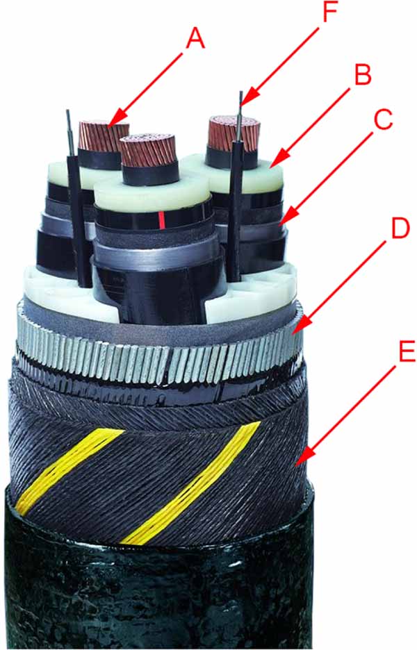
Standard image High-resolution imageThere are a variety of subsea power cables in terms of composition, length and diameter but despite the variation the basic function of conveying electric power remains the same [4]. They vary from 70 mm to 210 mm in diameter and are either alternating current (AC) or direct current (DC). The major differential factor when selecting between high voltage (HV) AC and HVDC is primarily the distance to be covered. For a route length less than 80 km the HVAC cable is more suitable, whilst distances over this are better suited to HVDC cables. There are several different designs of subsea power cables. Each cabling system is specially designed and optimised for purpose, making repairs and maintenance challenging, standardised cables are rare [5]. Some of the most common features for a standard, dry, subsea power cable are illustrated in figure 2 and described in table 1.

Figure 2. Key components of a typical three core, HVAC subsea power cable.
Download figure:
Standard image High-resolution imageTable 1. Key components of a subsea power cable.
| A | Copper conductors |
| B | XLPE insulation |
| C | Metallic water barrier |
| D | Steel wire armouring |
| E | Outer polypropylene sheath |
| F | Fibre optic cable |
Subsea cable failures and repairs have been a major concern within the industry, and this is dictating a demand for improved subsea cable condition monitoring and fault detection systems. Reported failure modes include [6]:
- (a)Cable design—unsuitable cable or cable accessories design.
- (b)External Damage—damage caused by movement of seabed sediment, scouring, instability of the cable and interaction with fishing gear and anchors.
- (c)Manufacturing—undetected flaws introduced during the cable manufacturing processes.
- (d)Installation—damage introduced during the installation processes due to human error, unsuitability of the installation spread or tools, incorrect cable handling, improper installation procedures and lack of experience of personnel.
Most static cable failures currently occur due to anchoring or fishing (trawling) damage; however, some previously installed cables are becoming exposed due to seabed movements [7–9].
In 2018 the Offshore Renewable Energy Catapult reported that the UK's operational offshore wind farms used 62 export cables totalling a length of 1499 km and over 1806 km of inter-array cables to transport 6.3 GW of generated power [2]. Of these a total of 43 array and export cable failures had been reported since 2007, with the most common cause of cable failure cited to be issues associated with manufacturing and/or installation. From 2014 to the end of 2017, recorded cable failures at UK offshore wind projects have led to a cumulative loss of power generation of approximately 1.97 TWh [10]. These values had increased to a total of 68 export cables totalling 1682 km and 2152 km of inter-array cables transporting nearly 8 GW of generation, over 50 failures recorded for fully commissioned sites by the end of 2019. This shows an increase of around 12% in export cables, 19% in inter array cables, 27% in generated power and 16% increase in reported failures. It should be noted that these figures relate to static subsea power cables.
Figure 3 shows the proportion of failure modes recorded for export and inter array cables in offshore wind farms between 2015–2019 [11]. New floating wind installations also have a demanding loading regime, which will require dynamic cables. Dynamic cable systems are still under development with no large-scale commercial farms in place (>100 MW), and only a few small scale installations at an early stage of commercialisation in operation (e.g. Hywind Scotland, 30 MW [12]; Kincardine, 50 MW [13]). Subsea cable integrity and repairs have been a major concern within the industry. With the recent announcement from The Crown Estate [14] outlining a potential 4 GW of floating wind in the Celtic Sea, improved subsea cable condition monitoring techniques and fault detection systems will be essential to support these efforts.

Figure 3. Recorded failure modes for export and inter array cables in offshore wind farms 2015–2019.
Download figure:
Standard image High-resolution imageFatigue failure of cables is not a new phenomenon, but with the advent of exposed sections of cable it is a key concern for dynamic systems [15, 16]. Low cycle fatigue in the lead alloy sheath of higher voltage subsea power cables has been evident from many years [17], with recent reports indicating an improvement on the fatigue performance of such a layer when integrated in a multi-layer cable structure compared to small scale fatigue tests on material samples for development of S-N curves [18]. Use of the lead alloy E as a waterproof sheath in dynamic subsea power cables is unlikely to be a suitable solution due to its propensity towards work hardening and eventual disintegration [15, 16]. Raoof and Davies [19] state that there is much evidence to indicate that the criterion of fatigue failure for spiral strands and ropes is more complex than that applied to continuous structures where crack length measurements or a simple observation of loss of integrity may suffice. Recent work has focussed on local numerical modelling of cable cross sections [20], and coupled global-local modelling [21, 22], to better understand the stresses in each layer and the effect on fatigue life of the cable. It is likely that the fatigue life of the cable as a complex composite structure may far exceed that of the individual component materials and associated S-N (or  -N) curves. Fatigue failure in dynamic cables may result from different failure modes such as bird caging, wear, and fretting damage between internal cable umbilicals [23]. Biofouling may also exacerbate fatigue failure of dynamic cables in the open ocean due to associated changes in the cable geometry, mass, and hydrodynamic properties [23–25].
Both dynamic and static cables can be tested in laboratory experimental test rigs, to characterise the overall properties and reliability of the cable. However, even under controlled conditions, it is not currently possible to determine the onset or progression of failure during the test. The damaged cables are typically dissected to facilitate a post-mortem inspection at the end of the test campaign. This approach does not facilitate direct identification and quantification of the failure mode [26, 27].
Current commercial state of the art monitoring technologies for subsea cables predominately focuses on the internal failure modes associated with partial discharge via online partial discharge monitoring and distributed strain and temperature measurements via embedded fibre optics [6, 28–30]. The existing fault detection methods heavily depend on thresholds and residual trace analysis. Based on industry standard fault location equipment and the knowledge of the operator, faults on subsea cables are often difficult to locate [7]. There are many fault diagnosis systems for subsea cables, which focus on internal failure modes due to partial discharge and localised heating from electrical overloading and/or degradation of internal insulation materials [31–34]. However, these systems are not able to predict the expected lifetime, of a cable section subjected to various wear-out mechanisms [35]. Recent advances include the CLEMATIS project [36] and distributed vibration sensing [37–39] both make use of the fibre optic bundles that are present in all cables that are used to detect major failures (anchor strike, installation issues); however, both are still, as yet, unable to detect smaller, fatigue related, failures, and also levels of movement. About 70% of failure modes in subsea power cables are not detected by currently installed state-of-the-art monitoring systems [7].
Non-destructive examination (NDE) methods exist for a range of end uses in many aspects of industry and research [40–47]. However, due to the complex layup of subsea power cables (with composite, plastic and metallic layers) no single technique is currently available that can accurately detect the occurrence, location and type of failure the cable experiences under dynamic loading. There is a need to develop a method for NDE of subsea power cables in marine renewable energy installations to determine the location, cause and type of fault to facilitate timely repair and minimise both the associated insurance claims and operation and maintenance costs.
Current practise for fatigue qualification of subsea power cables consists of mechanical testing, exposing the cable to a prescribed number of loading cycles (determined through use of industry standards, such as CIGRE TB 623 [48]), followed by electrical testing, and then physical dissection of the cable. Such a process merely indicates the presence of damage, if any, but does not provide information as to when and why the damage occurred. NDE methods will be essential at this stage of cable design, development, and qualification to improve understanding of failure modes and mechanisms of cables during prescribed fatigue testing in dry test rigs.
The aim of the work described in the present paper was to test and assess currently available NDE methods, used in other disciplines, for suitability in determining failure modes, mechanisms and locations on a dynamic subsea power cable under test at the Dynamic Marine Component (DMaC) facility in the University of Exeter. Three NDE methods were trialled, that had initially been identified as promising, on a cable under physical tests, namely: (a) thermography, (b) eddy current testing (ECT), (c) spread spectrum time domain reflectometry (SSTDR). The methods were assessed in several aspects:
- (a)what information could be obtained from both a static and oscillating cable,
- (b)how the results from one technique could potentially inform another technique,
- (c)if these techniques had the potential to be combined in the future to create a method NDE for dynamic subsea power cables that can not only be used in controlled experimental facilities, but also on location at wind farms to determine the location and type of fault occurring in a cable thereby facilitating operation and maintenance activities.
The paper is structured as follows. Section 2 introduces the general experimental setup for the cable test, section 3 gives an overview to the individual NDE techniques. Section 4 presents the monitoring results for all three NDE techniques.
2. Experimental cable testing
2.1. Experimental facility
The DMaC test facility is a purpose-built test rig that aims to replicate the forces and motions experienced by marine components in offshore applications. A schematic of the test rig is show in figure 4. The test rig consists of a linear hydraulic cylinder at the tailstock that applies the tension and compression forces or displacements. At the other end of the rig, the headstock with 3° of freedom can apply bending moments (torque) and angular displacements. The combination of forces and motions from the headstock and tailstock simulate the loads and displacements experienced by a floating body. The rig has a total length of 6 m and a maximum test bed length of 4.5 m; however, cable samples of any length can be tested with the extra cable extending out of the rig at the headstock.

Figure 4. Experimental facility—Dynamic Marine Component (DMaC) test rig.
Download figure:
Standard image High-resolution imageThe DMaC rig is capable of replicating dynamic tensile forces up to 20 te, static tensile forces up to 40 te, and displacements up to 1 m. The maximum bending angle at the headstock is ±30° for pitch and roll with up to 10 kNm of bending moment. The maximum torque or yaw is 10 kNm with an infinite rotational displacement. Components may also be submerged in fresh water to allow testing in a wet environment; sea water is not used to avoid the risk of corrosion. The above features allow dynamic testing of large-scale components under controlled conditions with realistic motion or load characteristics [49].
2.2. Cable specification
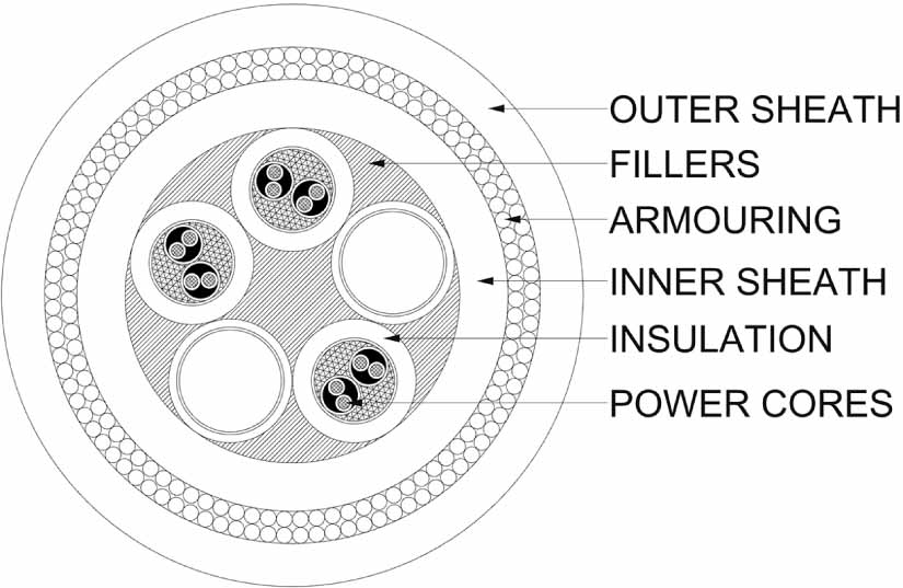
The cable used for this work was a typical subsea power umbilical with six, twin power cores surrounded by insulation, double steel wire armouring and plastic outer sheath. A schematic of the cable is shown in figure 5. Whilst the actual components of the cable may vary for each offshore renewable energy site and use, the construction, armouring and general properties are comparable. In this case, where NDE methods are being assessed for their practicability in monitoring of subsea power cables for offshore renewables, the cable provides a suitable basis for comparing the different techniques.

Figure 5. Cross-section of the subsea power umbilical under test.
Download figure:
Standard image High-resolution imageThe cable test section was 3.5 m in length and 108 mm outer diameter. The minimum breaking load is 100 kN, and the minimum bend radius is 2 m. The cable has an axial stiffness of 6.76 MN m−1 and a bending stiffness of 10 kNm2 [49].
2.3. Experimental set up
The cable was connected to the test rig at the headstock and the tailstock. At the headstock the cable was secured into a steel socket using resin, which then bolts onto the rig. At the tailstock, the cable was clamped between two cylindrical steel sections that were fitted with internal ribs to grip the cable. This clamp was connected to the main load cell through a pin joint connection, as illustrated in figure 6. The cable was not tested submerged in water, as this would have negated the use of two of the non-destructive testing (NDT) methods (thermography and ECT).

Figure 6. The cable set up for the experimental tests.
Download figure:
Standard image High-resolution imageDuring testing, the headstock was rotated on the lateral plane from 0°–25°, and tension was applied through the linear actuator in the range of 0–2.5 te. This magnitude of motions has previously been shown to be comparable to those experienced in the open ocean by this cable [49]. It should be noted, however, that the test parameters summarised in table 2 were intended to be exploratory, with the aim of assessing the three NDT methods for potential use in subsea cable monitoring, and a view to interrogate each more methodically in future. As such, the test regime was very fluid and different static and dynamic tests undertaken as results were assessed on site, and further investigation into various aspects appeared promising. Table 2 shows the cumulative range of tests carried out over the three NDT methods.
3. NDE methods
3.1. Thermography
Infrared thermography [50] is an NDE technique that is widely used in many fields, from medicine to engineering, for a wide range of purposes. In the aerospace industry it is frequently used for the inspection of large components such as aircraft structures, aero-engine parts, and spacecraft components. The technique can be applied to different materials including aluminium, composites and hybrid fibre metal laminates [51]. Thermography has also been developed for use in through life condition monitoring in the marine industry [52]. In this work both pulse thermography (PT) [53] and thermoelastic stress analysis (TSA) [54] were considered.
PT uses a short duration heat pulse, which heats the surface of the inspected specimens by radiative heat transfer. A thin layer at the surface of the specimen is instantaneously heated, the material conducts the heat in a direction normal to the inspected surface causing surface temperature decay which is monitored by an infrared detector, and the temperature evolution through time recorded [53]. PT relies on the difference of thermal properties between defective and non-defective regions to identify defects. PT is widely used in the aerospace industry as it is a full field technique and can rapidly inspect large areas. PT provides quantitative results, where the images can be post processed computationally to provide additional information such as defect size and depth [55]. PT has been used to inspect both composite materials and adhesively bonded joints, particularly for incidences concerning delamination and debonding [56]. All thermographic inspections of composite materials are limited in probing depth since they rely on heat conduction through a solid of low thermal diffusivity. Therefore, whilst existing thermographic techniques are considered capable of identifying the types of defects expected in maritime joints, the limited probing depth currently precludes their use.
TSA is a full-field technique that has seen application over the past several decades to a range of materials and components. Its application for damage detection in composites, materials and structures has been widely explored [57–60]; however, its application to the monitoring of the progression of fatigue cracks is a much more recent application [61, 62]. TSA is based on the coupling between the elastic deformation of a material and the heat energy developed in a material specimen subject to cyclic loading [54], known as the thermoelastic effect. Figure 7 shows a schematic of the procedure. The load is recorded from the test machine as an analogue output whilst the temperature is captured by the infrared camera in a sequence of images. Both the load and temperature signals are post processed to using a 'lock-in' procedure to provide a temperature change, ΔT, which is directly proportional to the stress change. Typically, TSA provides surface data but can detect damage (for example cracks) at various depths depending on the loading frequency and associated level of thermal response, recently demonstrated by Jiménez-Fortunato et al [63].

Figure 7. Thermography measurement schematic.
Download figure:
Standard image High-resolution imageThermal data was captured using a Telops MK3 infra-red camera from the cable undergoing cyclic loading in the DMaC rig and processed to provide TSA images. PT was facilitated using a Bowens flash unit to provide the heat pulse with thermal data capture using the Telops MK3 thermal camera. Figure 8 shows the thermography equipment set up on the cable under test in the DMaC test rig.

Figure 8. Pulse thermography set up on the cable under test in DMaC.
Download figure:
Standard image High-resolution image3.2. ECT
ECT is a well-established electromagnetic NDT technique, widely implemented in industry to detect damage or changes in the material properties of electrically conducting (typically metallic) components [64–66]. ECT plays an important role in numerous industries, especially in material coating, nuclear and oil & gas for detection of defects in metal pipelines [67–70]. Due to its high sensitivity to small surface defects, it is regularly used for the inspection of many safety-critical components such as aircraft engine & fuselage components.
Eddy-current NDT relies on the electromagnetic induction of electrical current in electrically conducting parts being tested. For this reason, it is typically used for the inspection of metals. The basic principle of the technique involves exciting a coil with alternative current, which generates a changing magnetic field around a coil. This changing magnetic field induces surface currents to flow in any electrically conducting material it penetrates via Faraday's law. The strength and density of these currents is dependent on the material properties of the specimen under test, including electrical conductivity, magnetic permeability, and the excitation frequency. Stronger eddy-currents in the specimen generate stronger magnetic fields of their own, which interact with the excitation coil and induce changes in the electrical properties of the coil. Therefore, any changes to the conductivity or permeability of the material are detected as a change in the electrical impedance of the coil. As such, an eddy current measurement is effectively a measure of changes in the effective conductivity and permeability of the test specimen [71].
In this study, ECT sensors were applied to the external circumference of a sub-sea cable under dynamic testing, and a differential measurement technique employed to evaluate whether changes in the properties of the cable architecture could be detected non-destructively. A bespoke set of sensor coils and electrical probe circuit was developed for the sub-sea table testing, figure 9. For the complex structure of the sub-sea cable under consideration, sensors were designed to generate eddy-current flow in the transverse direction across the direction of the steel wire armouring. This was to evaluate the cross-wire conductivity, and effective magnetic permeability which would vary as the armouring moved during cable oscillations.

Figure 9. Schematic of the ECT measurement instrumentation.
Download figure:
Standard image High-resolution imageThe differential sensor configuration was employed to measure the electromagnetic response of the cable rotating around the azimuthal axis. The two coils positioned next to each other along the cable axial direction and housed in a 3D-printed collar that was secured to the outside of the cable using Velcro straps, see figure 10. This housing was incrementally rotated around the cable in arc-length increments of 1 cm (equating to 10.58°). At each measurement position, 100 measurements were recorded and averaged.

Figure 10. Static rotation measurement configuration (left) and photo of sensor set-up (right).
Download figure:
Standard image High-resolution imageIn the configuration, shown in figure 10, both sensors were parallel and operating in differential mode, measuring local variations in the effective magnetic permeability and azimuthal current density generated in the cable armouring. This measurement depended on the amount of wire-to-wire contact between neighbouring steel wires and the maximum signals were observed when the difference between the two sensor coils was greatest. To test the response of the cable as a function of the dynamic movement of the cable, the sensors were re-distributed such that each coil covered one side of the cable along the axis of cable motion (see figure 9). This configuration allowed a differential measurement to be made between the extended and the contracted sides of the cable as it was rotated. This ensured that the maximum difference in effective permeability and azimuthal conductivity was measured.
3.3. SSTDR
The time domain reflectometry (TDR) technique is comparable to radar, whereby a pulse is sent out and a reflection is received and interpreted and can be used to detect changes in electrical cables [72]. The accuracy of TDR is impacted by other signals on the monitored cable, requiring the system to be powered down to carry out the test. SSTDR [73] is a combination of traditional TDR and spread spectrum techniques. Spread spectrum is a foundation of cellular phone communications, used to transmit small, but recognisable, signals in high noise environments. By combining spread spectrum with TDR, a significant breakthrough in being able to monitor and locate real-time changes in live electrical circuits has been achieved. SSTDR has some distinct advantages: It can be used on live electrical systems with minimal interference with signals already present in the system [74]. It has natural noise immunity [75] so experiences minimal interference from existing signals in the system or external electrical noise sources, and it possesses a dynamic frequency-domain bandwidth that can be varied by the modulation frequency [76]. Reported applications successfully demonstrate the detection and location of open and short circuits in aircraft, rail, and cable diagnostics (nuclear, subsea oil and gas, etc) [73, 77–79].
In this work, an SSTDR S100 unit was connected to two lines of the cable, by soldering a short leader wire onto the cores and then connecting this wire to the SSTDR unit. Vibrations applied to the wire connecting the unit and the cable (such as those from headstock rotation) lead to significant variation in data, therefore the S100 was securely attached to the headstock so that it experienced no relative forces and was only measuring the changes along the cable, figure 11.

Figure 11. SSTDR unit connected to the cable power cores.
Download figure:
Standard image High-resolution imageAs the cable was only a few metres long, the unit was unable to measure the primary reflection due to impedance changes, therefore measurements were dependent upon the secondary reflections found in the data, which occurred due to the far end of the cable being unterminated. This is not standard practise in real-world testing; however, the data is representative of how SSTDR technology would behave on a longer cable. Hard testing was also performed upon the wire to verify that the existing functionality of S100 units (hard fault detection and location) could be applied to this class of cable. The response of the cable was measured over various static and dynamic tests. The scan rate used was 16 Hz, and the frequency of the signal was 12 MHz and 24 MHz—both were assessed to determine their suitability in a noisy environment.
4. Results
4.1. Thermography
Despite the known limitations of thermography as a surface technique and concerns over the depth of detection of imperfections that would be possible, overall both TSA and PT showed promising results which indicate a potential new application for these techniques for assessment and monitoring of power cables under test in controlled conditions.
Figure 12 shows an image of the magnitude of the small temperature change, ΔT, extracted from the TSA processing for a 25° bend, and a 0.5 te axial load. It is possible to discern the helical pattern of one of the internal layers of the cable, even through the 10 mm thick outer plastic sheath.

Figure 12. TSA data from the cable under cyclic loading of 25 ° bend and 0.5 tonne axial load.
Download figure:
Standard image High-resolution imageThe thermal images captured during the pulse excitations were post-processed by averaging the first 20 images to obtain a 'noise-free' frame, as described by Ólafsson et al [80] The 'noise-free' frame was then subtracted from the whole data set. This process serves to remove most of the systematic error, associated with the high energy heat pulse. The thermal data was then smoothed temporally, pixel by pixel, using a technique known as thermal signal reconstruction [81] which fits a low order polynomial to the thermal decay by assuming it is exponential. Figure 13 shows the processed data, where the different materials in the cable sheath construction are apparent. There are some clear 'hot/cool spots' which emanate from small defects on the exterior of the cable.

Figure 13. Thermal data from pulse thermography.
Download figure:
Standard image High-resolution image4.2. ECT
The results obtained through azimuthal sensor rotation, static cable rotation, and dynamic cable rotation, are considered in this section.
Azimuthal sensor rotation
The magnitude and phase of the voltage ratio between the two coil sensors in the parallel configuration were normalised to the minimum ratio response. This is shown in figure 14 as a function of the polar angle of the differential sensor pair around the cable. A difference is due to a local variation in the wire-to-wire contact of the steel armouring beneath each sensor coil. From the overlapping data-points between 330°–0°, it can be observed that the measurement is repeatable for the static cable. Figure 14 indicates that the variations observed are therefore a function of the cable architecture, and not due to slight variations in the pressure applied to the sensor between each measurement.

Figure 14. Magnitude and phase of the normalised voltage ratio between coils for static azimuthal measurements.
Download figure:
Standard image High-resolution imageStatic cable rotation
The magnitude and phase of the voltage ratio between the two coil sensors in the opposing-hemisphere configuration (figure 9) are shown in figure 15. The results indicate changes in sensor response as the cable angle at the headstock was incrementally increased to 30° and then decreased to 21°.

Figure 15. Magnitude and phase of the voltage ratio between coils for static incrementally varied cable rotation angles.
Download figure:
Standard image High-resolution imageFurther data below 21° on the return to zero, were collected however a significant shift in response was measured and so was omitted from figure 15 to allow better visual analysis of measured incremental changes. The dramatic shift in response below 21° was possibly due to stick and slip behaviour in the steel armouring causing a large shift in the azimuthal current density and effective permeability on one side of the cable.
Dynamic cable rotation
Based on the results obtained for the static cable rotation measurements, the phase of the voltage ratio was used to monitor the dynamic motion of the cable, due to the greater sensitivity to changes in the cable architecture. Figure 16 shows the sensor phase response as a function of time, compared to the cyclic cable movement. The plots show the measurements for four separate dynamic motions, with respective rotation cycle periods and peak rotation amplitudes: A = (20 s, 5°), B = (10 s, 5°), C = (10 s, 10°) and D = (10 s, 15°).

Figure 16. Dynamic cable motion as a function of time, showing the cable rotation cycle compared to the phase response of the differential sensor. A = upper left, B = upper right, C = lower left, and D = lower right.
Download figure:
Standard image High-resolution image4.3. SSTDR
Due to the un-conventional cable attachment, there was a concern that testing performed on the wire may be detecting movement in the short leader cable instead of changes in the core of the test cable. To test this, the cable leading to the core was momentarily disconnected, and a bend test was performed. No changes were detected with the wire disconnected, suggesting that all changes observed did originate from the cable.
Fault detection
Figure 17 shows typical results from the SSTDR, when used for the intended purpose of locating hard faults along a wire:
- On the left graph, the blue line represents the baseline performed without fault and the red line is the system after creating the fault.
- On the right graph, the green line is showing the difference between the two lines on the left graph. The highest point represents the fault location.

Figure 17. Locating hard faults along a wire using SSTDR: baseline signal (blue) and signal with fault (red) on the left, and the difference between the base and signal with fault on the right. Relative impedance is shown on the y axis.
Download figure:
Standard image High-resolution imageThis testing is looking for smaller changes in impedance than would be typical for hard faults, so the typical amplitude changes were much closer to the noise level than typical testing. Typically, in onshore based industries, this type of testing can find a fault to within a metre in many kilometres of cable [73, 82]. In this case for the 3.5 m long cable, even with the noise level close to that of the signal, the fault was located to within a few centimetres of the actual position.
Sinusoidal bending, varied tension
Tension applied to the cable should slightly affect the impedance and can be detected on SSTDR traces for a given test. The cross-sectional area must reduce slightly for the volume of the conductor to remain consistent. Figure 18 shows the results of a cable rotation of 5° for three different tensions.

Figure 18. SSTDR sample #50 against time, for three different tension measurements.
Download figure:
Standard image High-resolution imageSinusoidal bending, various angles, fixed tension
Bending (past the minimum bend radius) is suspected to be one of the primary causes of cable degradation in dynamic umbilicals. As such, being able to detect repeated bending events would be advantageous for assessing cable damage. The SSTDR system not only detected faults in the cable, but also measured the movement of the cable. Figure 19 shows the measured electrical response when the end of the cable was oscillated with a 5 s period at 5°, 15° and 25°.

Figure 19. SSTDR response when the end of the cable was oscillated with a 5 s period at 5°, 15° and 25°.
Download figure:
Standard image High-resolution imageManual bending
To test how fine a rotation could be picked up, the cable was manually rotated by the rig operator instead of following a pre-set program. The results of this testing are shown in figure 20. From t = 0–80, rotation was performed with smooth stepping enabled, whereas from t = 80 onwards the rig was moved in (at least) single degree increments—the stair-stepping on the second half of this graph is indicative of this change. The movements could be clearly identified from the measurements alone.

Figure 20. Aggregated data, manual rotation of the headstock.
Download figure:
Standard image High-resolution imageFrequency component analysis
It is possible to identify different low-frequency components using discrete-time Fourier transforms on the returned data. An example of the use of this transform upon is shown in figure 21, with a Fourier transform run on both a 0.1 Hz and 0.5 Hz movement recorded at DMaC. When these samples were combined digitally, this action was able to isolate the two distinct frequency components as shown on the right-hand plot.

Figure 21. Fourier transforms of cable bend patterns at differing rates in the time domain (left) and frequency domain (right).
Download figure:
Standard image High-resolution imageFigure 22 illustrates data from a cable bending at two different rates (on the left-hand side) and that data processed using a Fourier transform to determine the frequency at which these events occurred (on the right hand side).

Figure 22. SSTDR data from cable bending at two different rates digitally combined (left) and the data processed using a Fourier transform (right).
Download figure:
Standard image High-resolution image5. Discussion
The results from each of the three monitoring techniques are discussed to provide an illustration of how improvements in subsea power cable monitoring could benefit the offshore renewable energy industry.
The thermal monitoring techniques, although limited by probing depth, did show information pertaining to cable defects and the underlying structure. TSA, in particular, indicated potential for use during experimental testing for the investigation of subsurface defects. Overall TSA worked reasonably well in terms of identifying the subsurface structure of the cable, with potential improvements to be gained in future if greater loads were applied. One prospective idea is to run a low frequency, AC current through the cable and utilise the heat the cable generates naturally in use as a means of detecting damage in the wires and or armour; a method of external excitation is proposed by Ólafsson et al [83] PT indicated areas of damage to the cable surface, and also the different materials used to make up the outer plastic sheath of the cable but did not manage to penetrate the outer sheath to provide an indication of structural response in the internal layers. However, knowledge of damage to the outer sheath is also integral as a point of reference for possible internal damage.
The key findings from the ECT assessment were during the static and dynamic cable rotation experiments. The results shown in figure 15, during the static cable rotation, demonstrate the ability of ECT to detect minor shifts in the configuration of the cable armouring and even highlights hysteresis between the increasing and decreasing rotation angles, indicating some 'memory' in the armature.
The result of the dynamic testing studies demonstrated that the sensor is capable of monitoring changes in the cable architecture as a function of time. The results also showed that slower motions with low cable rotations (top graphs in figure 16) could be monitored in real time, whilst more extreme angles of rotation at high cyclic rates produce more extreme responses with clear discontinuous points. These discontinuities indicate that the cable architecture may be responding in a different manner at faster cycle speeds, stick and slip between wires, such that more extreme interactions occur. The technique, even in this experimental setup, is capable of monitoring dynamic changes with suitable sensitivity. Future work is required to determine how these complex structures change under motion and how their structure affects the current density generated within the cables, and ultimately calibrate the measurements and data from ECT monitoring.
Due to the short length of cable under test, and concerns that the measured values would be close to noise from various electrical and mechanical operations, various initial tests were undertaken, and it was shown that all movements observed along the cable were due to electro-mechanical changes taking place in the umbilical. It was apparent that change in tension results in a small difference in measured SSTDR data (the aggregate difference between tension values is ∼250 units, whereas a 5° bend lead to a change of ∼1000 units). Cable rotation strongly affected the SSTDR trace, and the difference between 5°, 15° and 25° bend angles was clearly visible in the measured data. It is worth noting that some of the data appears to move in the negative direction, which was unexpected as it was anticipated that a bend in any direction would lead to a decrease in impedance when in practise the trace increased for one side and decreased for the other. However, this may simply be an artifact of the method used to gather data. The stair-stepping on the right-hand side of figure 20 suggests that the SSTDR data is accurate enough to detect the change in cable rotation to the nearest degree.
The frequency analysis, figure 22, has significant potential to be applied to real-life investigations to determine events the cable is exposed to in the open ocean. Such events may include normal wave and tidal loading, freak waves, or even vortex induced vibrations, which would provide essential data for understanding and estimating the fatigue life of the cable. The SSTDR technology has the potential to be able to isolate (and locate) these events in the field on live cables and would therefore provide valuable information to the companies responsible for maintaining the cables.
The Global Wind Energy Council predict that 469 GW of new wind energy capacity will be built globally by 2026 [84]. A further 235 GW of offshore wind energy is predicted to be installed by 2030, 16.5 GW of which will be floating offshore wind [85] (figure 23). Hence there will be a marked increase in demand for subsea power cables. Such an increase in demand comes with increased risks associated with installation, operation & maintenance, and repair. Cable monitoring systems that can operate on live cables remotely have the potential to reduce the cost and risk associated with personal transport. Successful monitoring techniques have the potential to mitigate costly insurance claims due to cable failure and enable much more efficient planning of maintenance operations.

Figure 23. Global offshore wind growth to 2030.
Download figure:
Standard image High-resolution image
Early-stage offshore wind farms have experienced considerable issues with exposed cables due to seabed movements. Reliable monitoring techniques that can be installed on live cables with minimal downtime offer a suitable mitigation technique to reduce some of those risks with existing and future installation. The NDE techniques assessed in this work, have the potential to monitor the cables in real-time and live stream the data back to shore for rapid assessment. Such information will be vital to monitor and ensure the integrity of the cables, and how soon stabilisation measures need to be implemented. They can also indicate if, when and where cable repairs need to be undertaken, and have the potential to significantly reduce the likelihood of wind farms going offline due to unexpected cable damage saving millions.
If successfully demonstrated in the field, SSTDR monitoring could be installed on live subsea cables for inherent condition monitoring and asset integrity assurance, without interrupting or interfering power production. The techniques are able to locate and quantify potential cable movement and identify cable faults, with the data live streamed back to shore. This information supports the wider 'digital twin' development [86], where a numerical model of the cable is maintained using the same conditions as that of the real cable. Successful development and wide-scale use of this novel sensing technology has the potential to contribute to cost reduction efforts for offshore assets, saving millions by avoiding offshore renewable energy arrays going offline due to cable failure. Assuming one export cable failure in the life of an average 200 MW wind farm (average capacity factor 0.4, 4 week lost revenue at 80£ MWh−1, £1.5 million cable repair cost) can be prevented, costs of up to £6 million would be avoided. For the UK's projected 40 GW capacity in 2030 this would amount to over £1 billion over the farm's lifetime.
6. Conclusions and further work
Subsea power cables are a critical component of the offshore renewable energy industry. With the advent of offshore wind moving into deeper waters and requiring floating platforms, power cables that can perform and survive in the energetic open ocean environment are required. Current commercial state-of-the-art monitoring techniques for subsea cables predominately focus on electrical parameters and the structural response of these highly complex structures is not well understood. Apart from fibre optic sensing, widely used for temperature monitoring, there is no technique currently available that can accurately predict the occurrence, location, and type of structural failure the cable experiences under dynamic loading regimes.
In this work three methods of NDE, all currently used in alternative industries, were assessed for their potential in monitoring the structural health of subsea power cables. The three methods were Thermography (both TSA and PT), ECT, and SSTDR. All three methods successfully detected various aspects of cable motion and structural response of a power cable under controlled static and dynamic experimental testing.
TSA was able to detect sub-surface structural interactions, and PT surface defects and material changes. ECT could recognise the stick-slip behaviour known to occur in the steel wire armouring, along with motions of the cable as it was dynamically moved in the test rig. SSTDR could detect core-to-core and core-to-sheath faults in the cable. It also captured the motion of the cable to within an accuracy of at least one degree. Frequency domain analysis of the SSTDR data also indicated it was possible to note when specific events happened to the cable, and at what length along the cable these occurred. Such events could range from day-to-day operational wave and tidal conditions, through to freak waves. High frequency events such as vortex induced vibrations may also be detected. Ultimately, improvements in the state of the art of cable monitoring have the potential to enhance NDE for subsea power cables. The examined techniques show considerable potential for use in the field of offshore renewable energy.
Further work will include further investigation and calibration of the NDE methods for use in real world situations and on live cables. The methods should be compared and combined with each other; some of those assessed, or other NDE methods, may have the potential to work together to provide a holistic view of the cable from various structural and electrical angles. Further investigation into other methods of NDE that may be utilised for structural health monitoring of subsea power cables should also be undertaken.
Acknowledgments
The work was funded through by the EPSRC Supergen Offshore Renewable Energy (ORE) Hub [EP/S000747/1].
Data availability statement
The data that support the findings of this study are available upon reasonable request from the authors.