
Building spatio-temporal knowledge graphs from vectorized topographic historical maps
Abstract
Historical maps provide rich information for researchers in many areas, including the social and natural sciences. These maps contain detailed documentation of a wide variety of natural and human-made features and their changes over time, such as changes in transportation networks or the decline of wetlands or forest areas. Analyzing changes over time in such maps can be labor-intensive for a scientist, even after the geographic features have been digitized and converted to a vector format. Knowledge Graphs (KGs) are the appropriate representations to store and link such data and support semantic and temporal querying to facilitate change analysis. KGs combine expressivity, interoperability, and standardization in the Semantic Web stack, thus providing a strong foundation for querying and analysis. In this paper, we present an automatic approach to convert vector geographic features extracted from multiple historical maps into contextualized spatio-temporal KGs. The resulting graphs can be easily queried and visualized to understand the changes in different regions over time. We evaluate our technique on railroad networks and wetland areas extracted from the United States Geological Survey (USGS) historical topographic maps for several regions over multiple map sheets and editions. We also demonstrate how the automatically constructed linked data (i.e., KGs) enable effective querying and visualization of changes over different points in time.
1.Introduction
Historical map archives contain valuable geographic information on both natural and human-made features across time and space [10,32] and are increasingly available in systematically acquired digital data formats [30,31]. The spatio-temporal data extracted from these documents are important since they can convey when, where and what changes took place [9]. For example, this type of data enables the detection of long-term changes in railroad networks or studying the evolution of wetlands within the same region over time and thus can support decision-making related to the development of transportation infrastructure or questions related to land conservation, landscape ecology, or long-term land development and human settlement. Many applications assessing geographic changes over time typically involve searching, discovering, and manually identifying, digitizing, and integrating relevant data. This is a difficult and laborious task that requires domain knowledge and familiarity with various data sources, data formats and working environments, and the task is often susceptible to human error [20].
Generally, there are two types of geospatial data, namely, raster data and vector data. Recent technological advances facilitate the efficient extraction of vectorized information from scanned historical maps [9,10,12,23,31]. Vector data provide a compact way to represent real-world features within Geographic Information Systems (GIS). Every geographic feature can be represented using one of three types of geometries: (i) points (depict discrete locations such as addresses, wells, etc.), (ii) lines (used for linear features such as roads, rivers, etc.) or (iii) polygons (describe enclosed areas like waterbodies, islands, etc.). This paper tackles the core problem of detecting how geometries change over time, focusing on linear and polygonal features.
Linked geospatial data has been receiving increased attention in recent years as researchers and practitioners have begun to explore the wealth of geospatial information on the Web [3,8,21]. In addition, the need for tracing geographic features over time or across documents has emerged for different applications [9]. Furthermore, growing attention has been paid to the integration and contextualization of the extracted data with other datasets in a GIS [1,2].
To better support analytical tasks and understand how map features change over time, we need more than just the extracted vector data from individual maps. We need to tackle the following challenges:
1. Entity generation and interlinking. Generate and interlink the geospatial entities (“building block” geometries originating from the vector data) that constitute the desired features (i.e., railroad lines or wetland areas) and can exist across map editions
2. External geo-entity linking. Contextualize and link the generated entities to external resources to enable data augmentation and allow users to uncover additional information that does not exist in the original map sheets
3. Representation. Represent the resulting data in a structured and semantic output that can be easily interpreted by humans and machines, and adheres to the principles of the Semantic Web
Previous work on creating linked data from historical geospatial information has focused on the problem of transforming a single instance of a map sheet or a formatted geospatial data source into Resource Description Framework (RDF) graphs [7,19,33]. However, this line of work does not address the issue of entity interlinking that is essential for building linked geospatial data for the task of change analysis with a semantic relationship between geospatial entities across map editions of the same region, which could be part of a large collection of topographic map sheets. Similar work is concerned with only a specific type of geometry, such as points, as in [2,34], or is limited to a specific physical feature (i.e. flooded areas [17] or wildfires [18]). Our work does not impose such limitations.
Our approach is not only helpful in making the RDF data widely available to researchers but also enables users to easily answer complex queries, such as investigating the interrelationships between human and environmental systems. Our approach also benefits from the open and connective nature of linked data. Compared to existing tools such as PostGIS,11 which can only handle queries related to geospatial entities and relationships within local databases, linked data can utilize many widely available knowledge sources in the Semantic Web, such as OpenStreetMap (OSM) [14], GeoNames [36], and LinkedGeoData [5], to enable rich semantic queries.
Providing contextual knowledge can help explain or reveal interactions of topographic changes to further spatio-temporal processes. For example, the external-linking enables augmentation of the contained geographic information with data from external KBs, such as historical population estimates. Once we convert the map data into linked data, we can execute SPARQL queries to identify the changes in map features over time and thus accelerate and improve spatio-temporal analysis tasks. Using a semantic representation that includes geospatial attributes, we can support researchers to query and visualize changes in maps over time and allow the development of data analytics applications that could have great implications for environmental, economic, or societal purposes.
This paper is based on our earlier conference and workshop papers [22,26]. The paper expands our methods to support polygon-based geographic features, elaborates on the details of the algorithms, and provides a more extensive evaluation of the methods. In addition, we use OpenStreetMap instead of LinkedGeoData as an external KB to obtain the most up-to-date information and provide a solution that does not depend on time-sensitive third-party data dumps.
1.1.Problem definition
The task we address here is as follows: Given geographic vector data extracted from multiple map editions of the same region, we aim to automatically construct a knowledge graph depicting all the geographic features that represent the original data, their relations (interlinks), and their semantics across different points in time. Using the constructed knowledge graph, we enable tackling more specific downstream analysis tasks. These may include the visualization of feature changes over time and the exploration of supplementary information (e.g., population data, elevation data, etc.) related to the region originating from an external knowledge base.
Fig. 1.
New Albany (OH) and Chicago (IL) railroad system maps in 1886 (left) and 1904 (right).
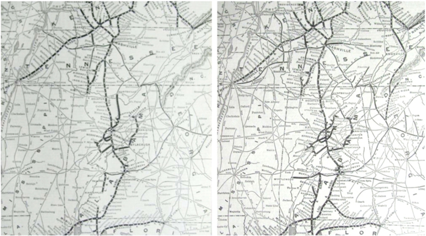
Fig. 2.
Visual representation of the change in the New Albany (OH) and Chicago (IL) railroad system between the years 1886 and 1904; additions are in red, removals are in blue.
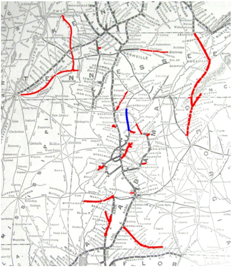
As an example, consider the maps in Fig. 1 where changes in the New Albany (OH) and Chicago (IL) railroad system have occurred between 1886 and 1904. Figure 2 shows the railroad line changes between the different map editions. Line segments that have been added are marked in red and line segments that have been removed are marked in blue. Assuming we have the data available as vector data (which can be generated from scanned maps using approaches such as in Duan et al. [12]), our task in such a setting would be to construct a knowledge graph describing the shared line segments that are shared across these maps or unique in individual maps with a conventional semantic representation for the railroad line segments in each map edition. This would include objects from a list of common geographic features (points, lines, or polygons), their geolocational details, and their temporal coverage to allow easy analysis and visualization.
1.2.Contribution
The overall contribution of this paper is a fully automatic end-to-end approach for building a contextualized spatio-temporal knowledge graph from a set of vectorized geographic features extracted from topographic historical maps. We tackle the core challenges we mentioned earlier by presenting:
1. An algorithm to identify and partition the original vector data into interlinked geospatial entities (i.e., “building block” geometries) that constitute the desired geographic features across map editions (entity generation and interlinking task)
2. A method to identify and retrieve geospatial entities from a publicly available knowledge base (external geo-entity linking task)
3. A semantic model to describe the resulting spatio-temporal data in a structured and semantic output that can be easily interpreted by humans and machines in a form of a knowledge graph that adheres to linked data principles (representation task)
We also present a thorough evaluation for each of the above and apply our method to five relevant datasets that span two types of geographic features: railroads (line-based geometry) and wetlands (polygon-based geometry), each resulting in an integrated knowledge graph. Finally, we make the source code, the original datasets, and the resulting data publicly available.22 We have also published the resulting knowledge graph as linked data, along with a designated SPARQL endpoint with compliant IRI dereferencing. The resulting knowledge graph characteristics are described in Table 1.
Table 1
Resulting knowledge graph characteristics
| SPARQL endpoint | https://linked-maps.isi.edu/sparql |
| Linked Data explorer | https://linked-maps.isi.edu |
| Size | 2 classes |
| 8 relations | |
| 630 nodes (340 non literals) | |
| 1514 edges |
1.3.Structure of paper
The rest of the paper is organized as follows. Section 2 presents our proposed approach and methods. Section 3 presents an evaluation of our approach by automatically building a knowledge graph for (i) a series of railroad networks from historical maps covering two different regions from different points in time, and (ii) a series of wetland data from maps covering three different regions from different periods. Section 4 reviews the related work. Section 5 concludes, discusses, and presents future work.
2.Approach to building spatio-temporal knowledge graphs
2.1.Overview of the approach
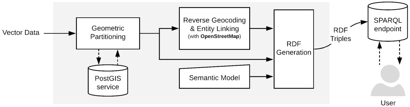
The proposed pipeline for the construction of the knowledge graph consists of several major steps as illustrated in Fig. 3. These steps can be summarized as follows:
1. Automatically partition the input geographic feature originating from the vector data into building block geometries (i.e., geospatial entities) using a spatially-enabled database service (e.g., PostGIS) (see Section 2.3).
2. Perform external entity linking by utilizing a reverse-geocoding service to map the geospatial entities to existing instances in an open knowledge base (e.g., OpenStreetMap) (see Section 2.4)
3. Construct the knowledge graph by generating RDF triples following a pre-defined semantic model using the data we generated in the previous steps (see Sections 2.5 and 2.6)
Once the RDF data is deployed, users can easily interact with the building block geometries (geospatial entities), the geographic features and metadata to perform queries (Section 2.7). These allow end-users to visualize the data and support the development of spatio-temporal downstream applications.
2.2.Preliminaries
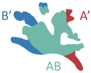
Before we discuss our proposed method, it is essential to define certain preliminaries and the terminology used in this paper. A geographic feature refers to a collection of geometries (points, lines, or polygons), which together represent an entity or phenomenon on Earth. In this paper, a geographic feature is represented using a collection of “building block” geometries. Given a set of geographic features pertaining to the same region from different points in time, each generated “building block” is essentially the largest geographic feature part that is either shared across different points in time or unique for a specific point in time. These blocks can be either lines or areas in the case of linear geographic features or polygon geographic features, respectively. For example, in Fig. 4a, A and B are line building blocks. Each building block may be decomposed into smaller building blocks. For example, if a part of A and B represents the same entity, A and B are decomposed into three building blocks: A’, B’, and AB. AB represents the shared geometry detected from A and B, and A’ and B’ represent the unique parts in A and B, respectively. Similarly, each color area in Fig. 5 (A’ in red, B’ in blue, and AB in green) is an area building block (giving a total of three building blocks). Each building block geometry is encoded as well-known text (WKT) representation (MULTILINE or MULTIPOLYGON textual format) and corresponds to a geospatial entity in our resulting KG.
Fig. 3.
Pipeline for constructing spatio-temporal linked data from vector data.
2.3.Generating building blocks and interlinking
The first task in our pipeline is the generation of building block geometries that can represent the various geographic features (e.g., railroad networks or wetlands) across different map editions in a granular and efficient fashion. This task can be classified as a common entity matching/linking and entity “partitioning” task. Given the geometries from different map editions of the same region, we want to identify which parts of those geometries coincide and thus represent the same parts of the feature. This allows us to generate building block geometries that are more granular and can be used to represent the common and the distinct parts (changes) of the geographic features.
Consider a simplified example consisting of linear features from two map editions (Fig. 4a), where line A is from an older map edition and line B is from the latest map edition with a part of the feature that has been changed. We split the lines into building block lines
Fig. 4.
Illustration of the geometry partitioning to building blocks for a line geometry: spatial buffers are used to identify the same line segments considering potential positional offsets of the data.
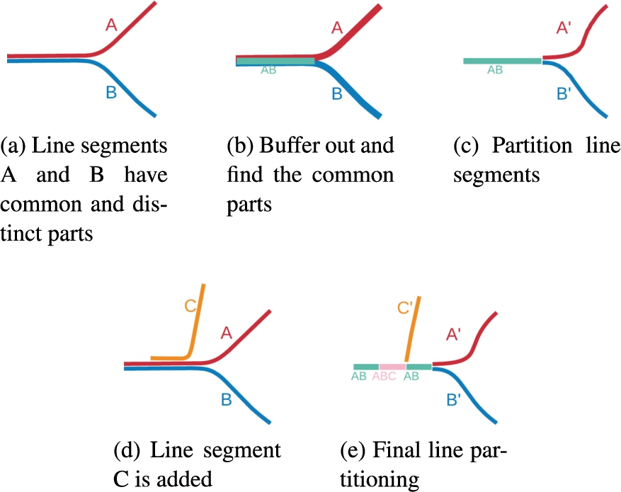
Fig. 5.
Illustration of a geometry partitioning result for a polygon geometry: each color represents a different building block. A single building block may contain disconnected areas.
As we mentioned in Section 2.1, we use a spatially-enabled database service to simplify handling data manipulations of geospatial objects. PostGIS is a powerful PostgreSQL extension for spatial data storage and query. It offers various functions to manipulate and transform geographic objects in databases. To handle our task efficiently and enable an incremental addition of map sheets over time, we implemented Algorithm 1. The algorithm performs the partitioning task by employing several PostGIS Application Programming Interface (API) calls over the geometries of our lines or polygons in the database. In the case of line geometries, we buffer each line segment to create two-dimensional areas before applying any geospatial operation described below.
Algorithm 1:
The feature partitioning and interlinking algorithm
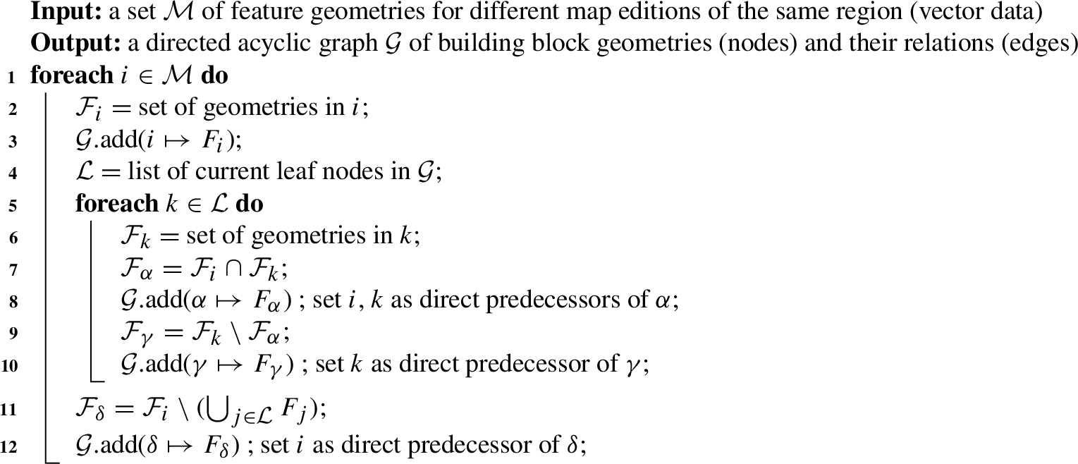
In detail, the procedure works as follows. The for loop in line 1 iterates over each of the map editions to extract the feature geometry (as seen in line 2 and stored in
1. For each “leaf” in
(a) Geometry intersection. k’s geometry is stored in
(b) Geometry difference (local “subtraction”). In line 9, we compute the geometry in k that is not in i, resulting in the geometry
2. Geometry union-difference (global “subtraction”). Once we finish going over the list of leaves, we compute the unique geometries that exist in i (the last added map edition in
In the worst-case scenario, graph
The relations between the nodes in graph
2.4.Reverse-geocoding and geo-entity linking
Volunteered geographic information platforms [13] are used for collaborative mapping activities with users contributing geographic data. OpenStreetMap (OSM) is one of the most pervasive and representative examples of such a platform and operates with a certain, albeit somewhat implicit, ontological perspective of place and geography more broadly. OSM suggests a hierarchical set of tags33 that users can choose to attach to its basic data structures to organize their map data. These tags correspond to geographic feature types that we will query (i.e., wetland, railroad, etc.).
Additionally, a growing number of OSM entities are being linked to corresponding Wikipedia articles, Wikidata [35] entities and feature identifiers in the USGS Geographic Names Information Service (GNIS) database. GNIS is the U.S. federal government’s authoritative gazetteer. It contains millions of names of geographic features in the United States.
Our proposed method for the enrichment of the generated geospatial entities (i.e., building block geometries) with an external resource is built upon a simple geo-entity linking mechanism with OSM. This is again a task of entity matching/linking; this time it is with an entity in an external knowledge base.
The method is based on reverse-geocoding, which is the process of mapping the latitude and longitude measures of a point or a bounding box to an address or a geospatial entity. Examples of these services include the GeoNames reverse-geocoding Web service44 and OSM’s API.55 These services support the identification of nearby street addresses, places, areal subdivisions, etc., for a given location.
Algorithm 2:
The geo-entity linking algorithm
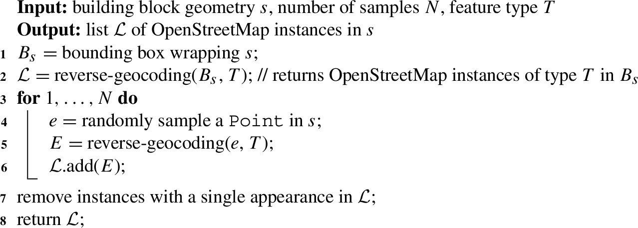
Fig. 6.
The method for acquiring external knowledge base instances.
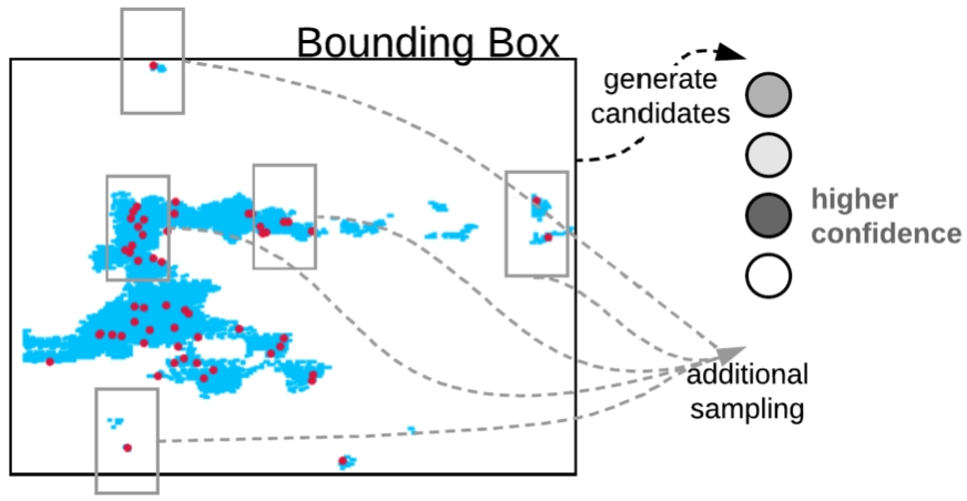
The geo-entity linking process is depicted in Algorithm 2 and illustrated in Fig. 6. We start with individual building block geometries of known type (T in Algorithm 2). In the case of the data we present later in the evaluation in Section 3, we start with the building blocks of geometries of railroads or wetlands (seen in blue in Fig. 6), so we know the feature type we are searching for. Each input building block geometry, s, is an individual node in graph
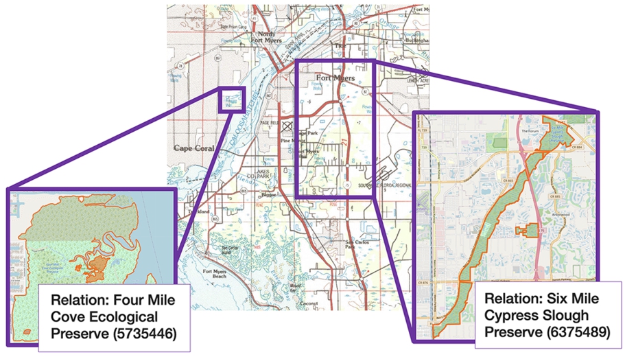
Figure 7 shows an example of a scanned topographic map (seen in the background), which we used to extract its corresponding wetland vector data, alongside two OSM instances detected using our geo-entity linking method. The labels in Fig. 7 (i.e., Four Mile Cove Ecological Preserve and Six Mile Cypress Slough Preserve) correspond to the name attribute of each entity. These labels are part of a set of attributes we use to augment our resulting data with information that did not exist in the original dataset.
The time complexity of Algorithm 2 depends on the number of samples N we choose and on the bounding box calculation. Each API call has a constant cost. As well, the bounding box calculation has a constant cost. Thus, the expected time complexity of Algorithm 2 is
Fig. 7.
An example of two OSM instances (enclosed in purple) and their name labels detected using our geo-entity linking method over a scanned topographic map (seen in the back).
2.5.Semantic model
As a generic model or framework, RDF can be used to publish geographic information. Its strengths include its structural flexibility, particularly suited for rich and varied forms for metadata required for different purposes. However, it has no specific features for encoding geometry, which is central to geographic information. The OGC GeoSPARQL [6] standard defines a vocabulary for representing geospatial data on the Web and is designed to accommodate systems based on qualitative spatial reasoning and systems based on quantitative spatial computations. To provide a representation with useful semantic meaning and universal conventions for our resulting data, we define a semantic model that builds on GeoSPARQL.
Our approach towards a robust semantic model is motivated by the OSM data model, where each feature is described as one or more geometries with attached attribute data. In OSM, relations are used to organize multiple nodes or ways into a single entity. For example, an instance of a bus route running through three different ways would be defined as a relation.
Figure 8 shows the semantic model we describe in this section. In GeoSPARQL, the class type geo:Feature represents the top-level feature type. It is a superclass of all feature types. In our model, each instance of this class represents a single building block extracted from the original vector data.
By aggregating a collection of instances of the class geo:Feature with a property of type geo:sfWithin we can construct a full representation for the geometry of a specific geographic feature in a given point in time. Similarly, we can denote the decomposition to smaller elements using the property geo:sfContains). The use of these properties enables application-specific queries with a backward-chaining spatial “reasoner” to transform the query into a geometry-based query that can be evaluated with computational geometry. Additionally, we use the property geo:sfOverlaps with subjects that are instances from OSM to employ the Web as a medium for data and spatial information integration following linked data principles. Furthermore, each instance has at least one property of type dcterms:date to denote the different points in time in which the building block exists. Each of the aforementioned properties has a cardinality of 1:n, meaning that multiple predicates (relations) of this type can exist for the same building block. The property dcterms:created is used to denote the time in which this building block was generated. dcterms stands for the Dublin Core Metadata Initiative66 metadata model, as recommended by the World Wide Web Consortium (W3C).77
Fig. 8.
Semantic model for the linked data. Nodes cardinality is shown in blue next to each edge.
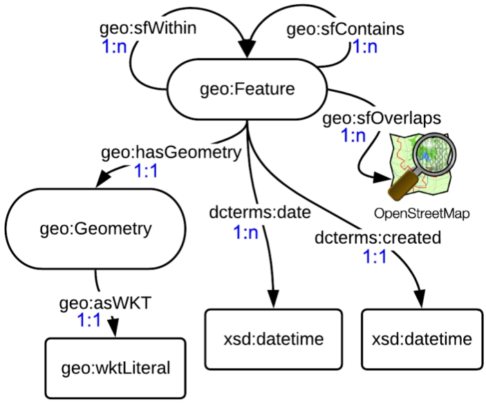
Fig. 9.
Mapping of the generated spatio-temporal data into the semantic model.
Complex geometries are not human-readable as they consist of hundreds or thousands of coordinate pairs. Therefore, we use dereferenceable URIs to represent the geospatial entity instead. Using a named node in this capacity means that each entity has its own URI as opposed to the common blank-node approach often used with linked geospatial entities. Each URI is generated using a hash function (the MD5 message-digest algorithm, arbitrarily chosen) on a plain-text concatenation of the feature type, geometry, and its temporal extent, thus providing a unique URI given its attributes. The geometry contains absolute coordinates, thus rules out the possibility of hash clashes. Each building block instance (geospatial entity) holds a property of type geo:hasGeometry with a subject that is an instance of the class geo:Geometry. This property refers to the spatial representation of a given feature. The class geo:Geometry represents the top-level geometry type and is a superclass of all geometry types.
In order to describe the geometries in a compact and human-readable way we use the WKT format for further pre-processing. The geo:asWKT property is defined to link a geometry with its WKT serialization and enable downstream applications to use SPARQL graph patterns.
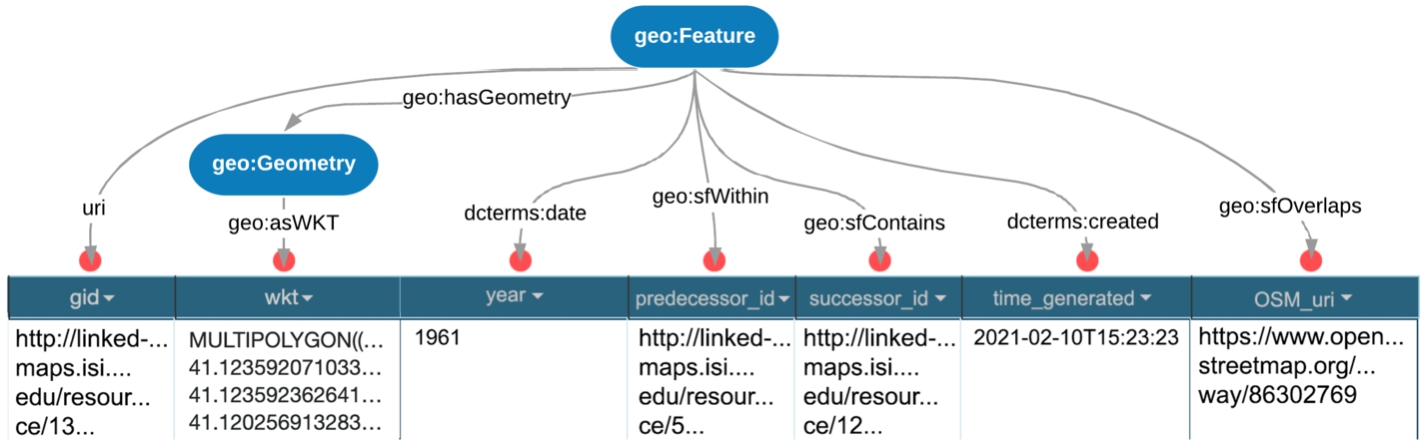
Figure 9 shows how the spatio-temporal data, resulting from the previous steps, is mapped into the semantic model (from Fig. 8) to generate the final RDF graph. The first column, titled gid, corresponds to the local URI of a specific node (building block geometry). The columns titled predecessor_id and successor_id correspond to the local URIs of the nodes composed-of and composing the specified gid node, respectively. All the three node entities are of type geo:Feature. The data in the wkt column contains the geometry WKT representation. It is linked to the building block node via an entity of type geo:Geometry, as we described above. The rest of the attributes (year, time_generated, and OSM_uri) are stored as literals, following the semantic model we presented in Fig. 8.
2.6.Incremental linked data
Linked Data technologies can effectively maximize the value extracted from open, crowdsourced, and proprietary big data sources. Following the data extraction and acquisition tasks described in Sections 2.3 and 2.4, and the semantic model described in Section 2.5, we can now produce a structured standard ontologized output in a form of a knowledge graph that can be easily interpreted by humans and machines, as linked data. In order to encourage reuse and application of our data in a manageable manner, we need to make sure that the linked data publication process is robust and maintainable.
This hierarchical structure of our directed acyclic graph
The approach we present is complete and follows the principles of Linked Open Data by:
1. Generating URIs as names for things, without the need to modify any of the previously published URIs once further vector data from the same region is available and processed
2. Maintaining existing relations (predicates) between instances (additional relations may be added, but they do not break older ones)
3. Generating machine-readable structured data
4. Using standard namespaces and semantics (e.g., GeoSPARQL)
5. Linking to additional resources on the Web (i.e., OpenStreetMap)
2.7.Querying
The semantic model presented in Section 2.5 and its structure provide a robust solution enabling a coherent query mechanism to allow a user-friendly interaction with the linked data.
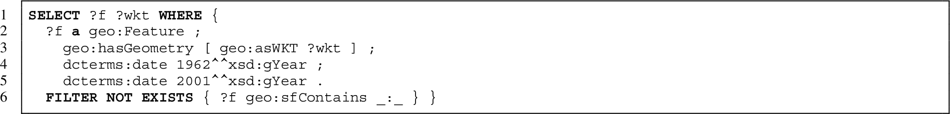
In order to elaborate on the query construction idea, we describe the elements that are needed for a general query “skeleton” from which we can establish more complicated queries to achieve different outcomes as required. Listing 1 shows a query (i.e., the “skeleton” query) that retrieves all the leaf node building blocks (i.e., the most granular building blocks). As shown in Listing 1, we first denote that we are interested in a geo:Feature that has a geometry in WKT format which gets stored in the variable ?wkt as shown in lines 3–4 (the variable we visualize in Figs 14, 15, 16, and 17). Line 5 restricts the queried building blocks (geo:Features) to leaf nodes only (in graph
Listing 1.
Our SPARQL query “skeleton”
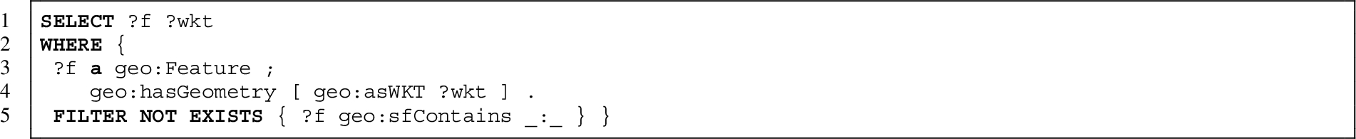
This is important due to the way graph
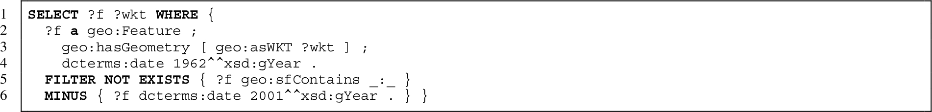
If, for example, we are interested to see the entire geographic feature in a specific point in time, we can add the clause {?f dcterms:date <...> .} inside the WHERE block (lines 2–5). If we are interested to see the changes from a different time, we can add an additional clause {MINUS { ?f dcterms:date <...> . }} as well. The syntax and structure of the query allows an easy adaptation for additional tasks such as finding the distinct feature parts from a specific time or finding the feature parts that are shared over three, four or even more points in time or map editions. The nature of our knowledge graph provides an intuitive approach towards writing simple and complex queries.
Fig. 10.
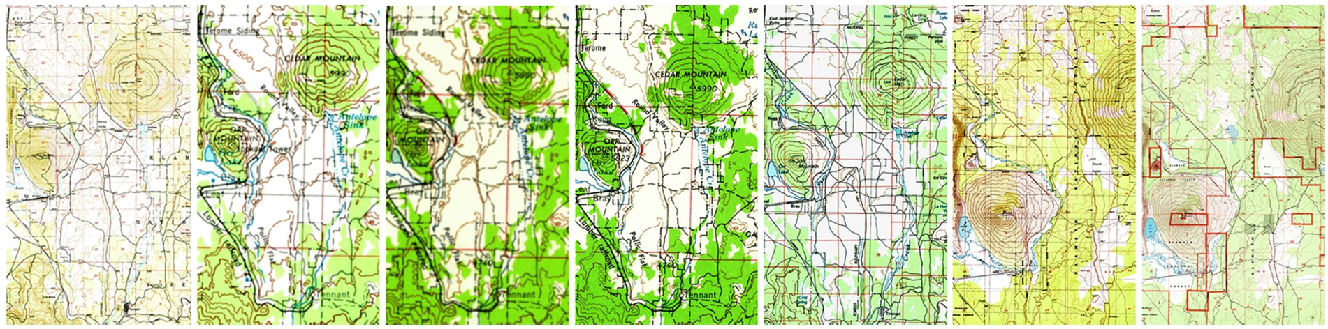
Historical maps of Bray, California from 1950, 1954, 1958, 1962, 1984, 1988 and 2001 (left to right, respectively).
3.Evaluation
We evaluate and analyze our methods using qualitative and quantitative methods over two types of geographic features: railroads (line-based geometry) and wetlands (polygon-based geometry). In this section, we present the results, measures, and outcomes of our pipeline when executed on the following datasets:
Railroad data We tested two datasets of vector railroad data (encoded as MULTILINEs) extracted from the USGS historical topographic map archive,8899 using the extraction methods of Duan et al. [12]. Each dataset covers a different region and includes map sheets for different points in time. The railroad data originates from a collection of historical maps for:
1. Bray, California (denoted as CA) from the years 1950, 1954, 1958, 1962, 1984, 1988, and 2001 (the original raster maps are shown in Fig. 10).
2. Louisville, Colorado (denoted as CO) from the years 1942, 1950, 1957 and 1965.
Wetland data We tested three datasets of vector wetland data (encoded as MULTIPOLYGONs) that were similarly extracted from the USGS historical topographic map. Again, each of these map sheets covers a different region and spans different points in time. The wetland data originates from a collection of historical maps for:
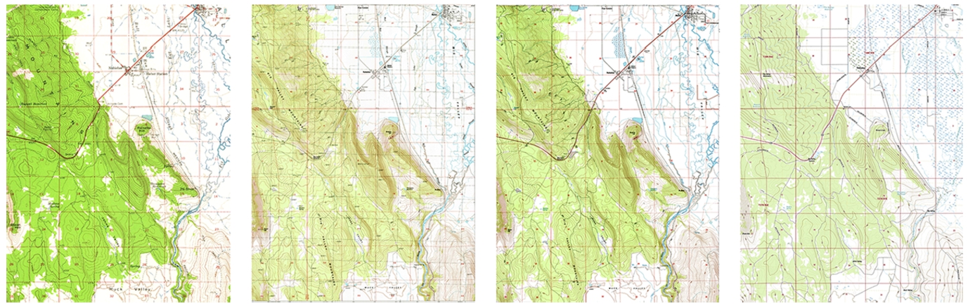
1. Bieber, California (denoted as CA) from the years 1961, 1990, 1993, and 2018 (the original raster maps are shown in Fig. 11).
2. Palm Beach, Florida (denoted as FL) from the years 1956, 1987 and 2020.
3. Duncanville, Texas (denoted as TX) from the years 1959, 1995 and 2020.
Fig. 11.
Historical maps of Bieber, California from 1961, 1990, 1993 and 2018 (left to right, respectively).
Our primary goal in this section is to show that our proposal provides a complete, robust, tractable, and efficient solution for the production of linked data from vectorized historical maps.
Table 2
Partitioning statistics for CA railroads
| Year | # vecs | Runtime (s) | # nodes |
| 1954 | 2382 | <1 | 1 |
| 1962 | 2322 | 36 | 5 |
| 1988 | 11134 | 1047 | 11 |
| 1984 | 11868 | 581 | 24 |
| 1950 | 11076 | 1332 | 43 |
| 2001 | 497 | 145 | 57 |
| 1958 | 1860 | 222 | 85 |
Table 3
Partitioning statistics for CO railroads
| Year | # vecs | Runtime (s) | # nodes |
| 1965 | 838 | <1 | 1 |
| 1950 | 418 | 8 | 5 |
| 1942 | 513 | 5 | 8 |
| 1957 | 353 | 4 | 10 |
Table 4
Partitioning statistics for CA wetlands
| Year | # vecs | Runtime (s) | # nodes |
| 1961 | 12 | <1 | 1 |
| 1993 | 17 | <1 | 5 |
| 1990 | 27 | 6 | 11 |
| 2018 | 9 | 6 | 24 |
3.1.Evaluation on the feature partitioning
In order to evaluate the performance of this task, we look into the runtime and the number of generated nodes (in graph
As seen in Tables 2, 3, 4, 5 and 6, we observe that for both types of geographic features, the building block geometries extracted from these maps vary in terms of “quality”. That is, they have a different number of vector lines that describe the geographic feature and each one has a different areal coverage (the bounding box area for each feature geometry is reported in Table 7). This is caused by the vector extraction process and is not within the scope of this paper. We also acknowledge that the quality and scale of the original images used for the extraction affects these parameters, but we do not focus on such issues. We treat these values and attributes as a ground truth for our process.
First, we note that the growth of the number of nodes in graph
Table 5
Partitioning statistics for FL wetlands
| Year | # vecs | Runtime (s) | # nodes |
| 1987 | 184 | <1 | 1 |
| 1956 | 531 | 180 | 5 |
| 2020 | 5322 | 1139 | 13 |
Table 6
Partitioning statistics for TX wetlands
| Year | # vecs | Runtime (s) | # nodes |
| 1959 | 8 | <1 | 1 |
| 1995 | 6 | <1 | 5 |
| 2020 | 1 | 1 | 10 |
Table 7
Geo-entity linking results; area is in square kilometers
| Area | Precision | Recall | |||
| Railroads | CA-baseline | 420.39 | 0.193 | 1.000 | 0.323 |
| CA | 0.800 | 0.750 | 0.774 | ||
| CO-baseline | 132.01 | 0.455 | 1.000 | 0.625 | |
| CO | 0.833 | 1.000 | 0.909 | ||
| Wetlands | CA-baseline | 224.05 | 0.556 | 1.000 | 0.714 |
| CA | 1.000 | 1.000 | 1.000 | ||
| FL-baseline | 27493.98 | 0.263 | 1.000 | 0.417 | |
| FL | 0.758 | 0.272 | 0.400 | ||
| TX* | 16.62 | – | – | – |
These results are not surprising because “leaves” in the graph will only be partitioned in case it is “required,” that is, they will be partitioned to smaller unique parts to represent the geospatial data they need to compose. With the addition of new map sheet feature geometries, we do not necessarily add unique parts since changes do not occur between all map editions. This shows that the data processing is not necessarily becoming more complex in terms of space and time, thus, providing a solution that is feasible and systematically tractable.
Additionally, by comparing the first three rows in Tables 2 and 5, we notice that the computation time over a polygon geometry is significantly slower than that of a buffer-padded line geometry. This is despite the railroads having a larger number of feature vectors. Further, by examining Tables 4, 5 and 6, we notice that a bigger number of feature vectors in the case of a polygon geometry causes a significant increase in processing time. These observations are predictable, as the computation time is expected to grow when dealing with more complex geometries like polygons covering larger areas that may include several interior rings in each enclosed exterior (similar to “holes in a cheese”), compared to the simple buffer-padded line geometries (sort of a “thin rectangle”).
3.2.Evaluation on geo-entity linking
In the process of linking our data to OpenStreetMap, we are interested in the evaluation of the running time and correctness (precision, recall, and F1, which is the harmonic mean of precision and recall) of this task.
As we expected, the running time is strongly dependent on the number of nodes in graph
Fig. 12.
Screenshot of a wetland instance on OpenStreetMap matching an active area corresponding to an instance we generated from the CA wetland data.
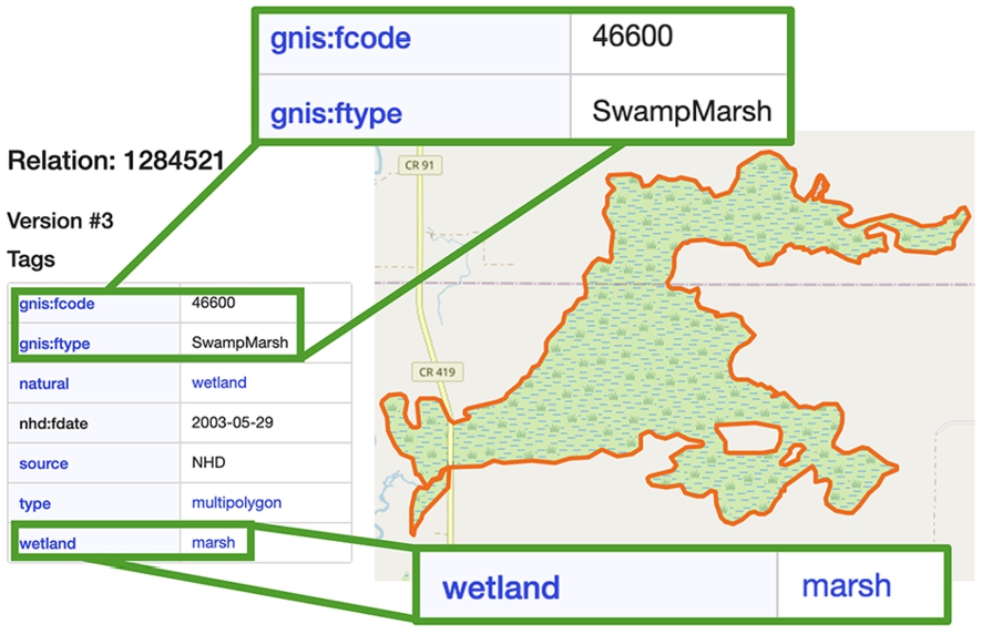
Fig. 13.
Screenshot of a railroad instance on OpenStreetMap matching an abandoned rail segment corresponding to an instance we generated from the CA railroad data.
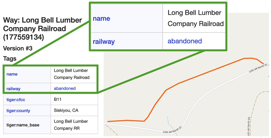
Due to the absence of a gold standard for this mapping task, we had to manually inspect and label the sets of instances found in each bounding box that we query for each building block geometry. The measure we present here is in terms of entity (instance) coverage. Precision and recall are calculated according to the labeled (type) instances that are available on OpenStreetMap and make up the inspected geographic feature (i.e., railroad or wetland). Figures 12 and 13 show an example of such instances, with their corresponding tags in OSM’s graphic interface. Figure 12 shows a wetland instance on OSM marked as a SwampMarsh (with its corresponding GNIS code) and matching an active wetland area in our data (a common building block from all the editions of the CA wetland data). Figure 13 shows a railroad instance on OSM marked as abandoned and matching an abandoned railroad segment in our data (a unique building block from the 1950 edition of the CA railroad data). This shows our ability to enrich and link our graph to external resources on the Web.
We have set up a baseline for comparison with our geo-entity linking method. The baseline approach returns the set of all instances found in the bounding box. This is the list of candidates we generate in the first step of our method, without the additional sampling and removal steps we have described in Section 2.4.
The precision, recall, and
Due to the varying geometries, areal coverage, and available data in the external knowledge base for each region, and as expected, our measure shows different scores for each dataset. In 3 out of 4 datasets, our method achieves much higher
3.3.Evaluation on querying the resulting data
We execute several query examples over the knowledge graph we constructed in order to measure our model in terms of query time, validity, and effectiveness. For the generated railroad data, we had a total of 914 triples for the CA dataset and 96 triples for the CO dataset. For the wetland data, we had a total of 270 triples for the CA dataset, 149 for the FL dataset, and 85 for the TX dataset.
Larger areas do not necessarily mean that we will have more triples. The number of triples depends on the geometry similarity and difference in the given data. Despite the FL wetland data covering a significantly larger area than other datasets, it did not cause notable triples growth or query performance degradation, as we show in Table 8.
The generated RDF triples would be appropriate to use with any Triplestore. We hosted our triples in Apache Jena.1010 Jena is relatively lightweight, easy to use, and provides a programmatic environment.
Table 8 shows the query-time performance results (average, minimum and maximum). In the first type of query we want to identify the feature parts that remain unchanged in two different map editions (different time periods) for each region (e.g., Listing 2). Each row with a label starting with SIM- in Table 8 corresponds to this type of query (the label suffix determines the tested region). We executed a hundred identical queries for each feature type and each area across different points in time to measure the robustness of this type of query.
We repeated the process for a second type of query to identify the parts of the feature that were removed or abandoned between two different map editions for each region (i.e., Listing 3). Each row with a label starting with DIFF- in Table 8 corresponds to this type of query.
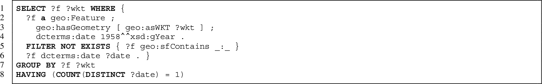
The third type of query retrieves the parts of the feature that are unique to a specific edition of the map (i.e., Listing 4). Each row with a label starting with UNIQ- in Table 8 corresponds to this type of query.
Table 8
Query time statistics (in milliseconds)
| avg | min | max | ||
| Railroads | SIM-CA | 12 | 10 | 18 |
| SIM-CO | 11 | 9 | 20 | |
| DIFF-CA | 10 | 8 | 20 | |
| DIFF-CO | 10 | 9 | 14 | |
| UNIQ-CA | 14 | 8 | 28 | |
| UNIQ-CO | 15 | 9 | 17 | |
| Wetlands | SIM-CA | 22 | 18 | 34 |
| SIM-FL | 35 | 18 | 55 | |
| SIM-TX | 21 | 12 | 44 | |
| DIFF-CA | 25 | 16 | 43 | |
| DIFF-FL | 32 | 18 | 60 | |
| DIFF-TX | 21 | 11 | 30 | |
| UNIQ-CA | 24 | 18 | 44 | |
| UNIQ-FL | 48 | 38 | 73 | |
| UNIQ-TX | 14 | 12 | 40 |
Listing 2.
Query similar feature geometries in both 1962 and 2001
Listing 3.
Query feature geometries present in 1962 but not in 2001
Listing 4.
Query unique feature geometries from 1958
Looking at Table 8, we notice that the average query times are all in the range of 10–48(ms) and do not seem to change significantly with respect to the number of map editions we process or the complexity of the query we compose. The query time results corresponding to the wetland data are slightly slower, but not significantly, comparing to the railroad data. This may be explained by the longer literal encoding of the WKT geometry for polygons, thus slower retrieval time comparing the line encoding.
Fig. 14.
Example of railroad system changes over time: the parts of the railroad that are similar in 1962 and 2001 are marked in red.
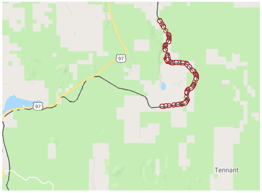
Fig. 15.
Example of railroad system changes over time: the parts of the railroad that are present in 1962 but are not present in 2001 are marked in blue.
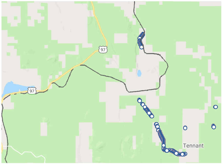
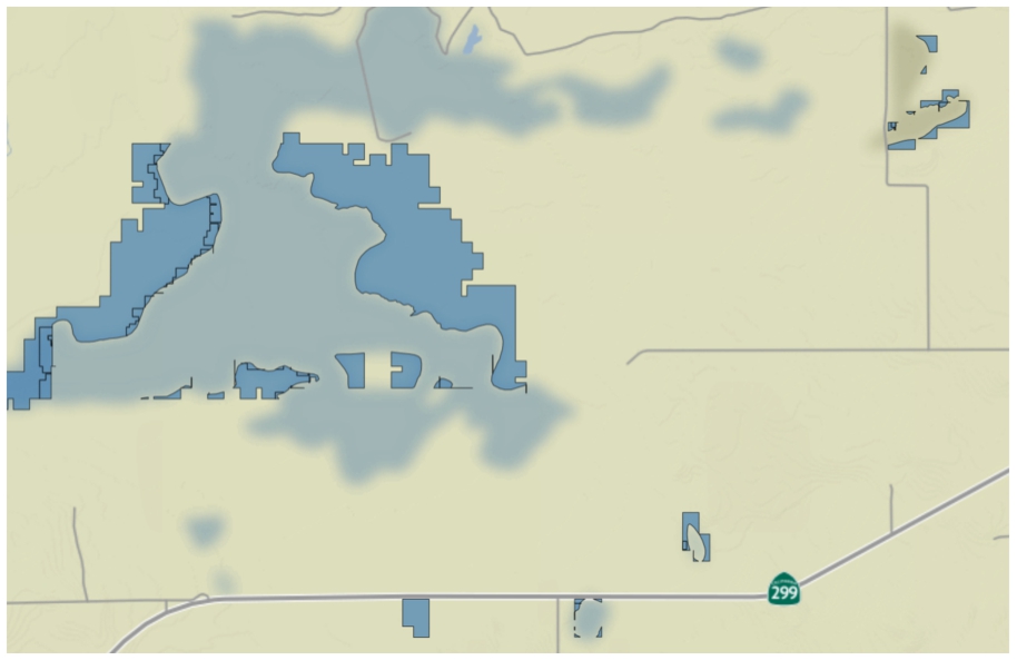
In order to evaluate the validity of our graph we observe the visualized results of the query presented in Listing 2 when executed over the CA railroad data, which are shown in Fig. 14. The figure shows in red the unchanged building block geometries between the years 1962 and 2001. We notice that the geometries we retrieve qualitatively match what we observe in the original vector data (the line marked in black over the maps in Figs 14 and 15 represents the current railway, which has not changed since 2001). The results of the query presented in Listing 3 are shown in Fig. 15, again, when executed over the CA railroad data. Figure 15 shows in blue the parts of the railroad that were abandoned between 1962 to 2001. Comparably, we perform a similar type of query and visualization for the CA wetland data, between the years 1961 and 2018. Figure 16 shows the similar parts in both editions (in red). Figure 17 shows the parts of the wetland (swamp) that were present in 1961 but are not present in 2018 (in dark blue). Again, this matches our qualitative evaluation based on the original vector files (the light blue marks that are part of the map’s background depict the current swamp, thus validating our results qualitatively).
Fig. 16.
Example of wetland changes over time: the parts of the Big Swamp in Bieber (CA) that are similar in 1961 and 2018 are marked in red.
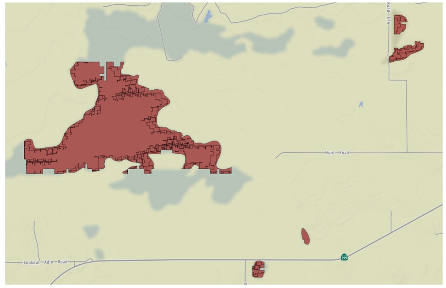
Fig. 17.
Example of wetland changes over time: the parts of the Big Swamp in Bieber (CA) that are present in 1961 but are not present in 2018 are marked in dark blue, emphasizing its decline throughout time.
The query results above establish high confidence in our model, showing that we can easily and effectively answer complex queries in a robust manner. Overall, we demonstrated that our approach and the proposed pipeline can be effectively used to automatically construct effective and contextualized open KGs and linked data from historical and contemporary geospatial data.
4.Related work
Much work has been done on mapping geospatial data into RDF graphs. Kyzirakos et al. [19] developed a semi-automated tool for transforming geospatial data from their original formats into RDF using R2RML mapping. Usery et al. [33] presented a method for converting point and other vector data types to RDF for supporting queries and analyses of geographic data. The transformation process presented in these papers does not address linking the data across multiple sources or linking the source data with additional knowledge bases on the Semantic Web as described in this paper.
Annotating geospatial data with external data on the Web is used for contextualization and the retrieval of relevant information that cannot be found in the source data. This line of research has been addressed in different studies. Vaisman et al. [34] studied the problem of capturing spatio-temporal data from different data sources, integrating these data and storing them in a geospatial RDF data store. Eventually, these data were enriched with external data from LinkedGeoData [5], GeoNames [36], and DBpedia [4]. Smeros et al. [29] focus on the problem of finding semantically related entities lying in different knowledge bases. According to them, most approaches on geo-entity linking focus on the search for equivalence between entities (same labels, same names, or same types), leaving other types of relationships (e.g. spatial, topological, or temporal relations) unexploited. They propose to use spatio-temporal and geospatial topological links to improve the process.
The discovery of topological relations among a simplified version of vector representations in geospatial resources has been studied as well. Sherif et al. [28] presented a survey of 10 point-set distance measures for geospatial link discovery. SILK [29] computes topological relations according to the DE-9IM [11] standard. In contrast, RADON [27] is a method that combines space tiling, minimum bounding box approximation, and a sparse index to calculate topological relations between geospatial data efficiently. These approaches work on matching geometry to integrate vector data from two sources in a single matching process. In contrast, our approach can systematically match multiple vector datasets iteratively without performing duplicate work.
Current work on geospatial change analysis spans the construction of geospatial semantic graphs to enable easier search, monitoring and information retrieval mechanisms. Perez et al. [25] computed vegetation indexes from satellite image processing and exposed the data as RDF triples using GeoSPARQL [6]. The changes in these indexes are used to support forest monitoring. Similar to that approach, Kauppinen et al. [16] collected statistical data from open data sources to monitor the deforestation of the Amazon rainforest by building temporal data series translated into RDF. Kyzirakos et al. [18] used open knowledge bases to identify hot spots threatened by wildfire. However, this line of work does not address an incremental process of geospatial change over time. In this paper, we incorporate a temporal dimension to the geospatial semantic graphs and present a pipeline for an automatic incremental geographic feature analysis over time.
5.Discussion and future work
With the increasing availability of digitized geospatial data from historical map archives, better techniques are required to enable end-users and non-experts to easily understand and analyze geographic information across time and space. Existing techniques rely on human interaction and expert domain knowledge. In this paper, we addressed this issue and presented an automatic approach to integrate, relate and interlink geospatial data from digitized resources and publish it as semantic-rich, structured linked spatial data in a form of a knowledge graph that follows the Linked Open Data principles.
The evaluation we presented in Section 3 shows that our approach is feasible and effective in terms of processing time, completeness and robustness. The partitioning process runs only once for newly added resources, and does not require re-generation of “old” data since our approach is incremental. In case a new map edition emerges for the same region, we only need to process the newly added geometry. Thus, data that has been previously published will continue to exist with a proper URI and will be preserved over time.
In a scenario that includes contemporary maps that change very quickly, we expect our method to require longer computation time, due to an increased number of computations, but would still be tractable with respect to the changes happening in the map geometries. As we mentioned in Section 2.3, the breakdown of the building block geometries depends on the complexity of the actual changes in the original topographic map. Further, the quality and level of detail of the original vector data play a significant role in the final RDF model as we have observed in Section 3.1.
Further, one may consider cases where a feature changes its very type over time. For example, a large body of water drying out to become represented as a line, or a river causing a flood and generating a polygonal feature. In such a case, we would determine that the feature has either disappeared or came into existence.
Our approach has several limitations, one of them is in a form of a hyper-parameter that governs the buffer size we use in the process of the partitioning of the geometries to smaller building block geometries in the case of line geometry. We currently set this parameter manually but we believe such parameter can be learned from the data or estimated using some heuristics with respect to additional attributes such as the area of the geometric object and the quality of the original vector data extraction. Additionally, it is worth mentioning that the reverse-geocoding API imposes another limitation. The API requires input in the form of an unrotated bounding box, which does not match the shape of the geo-entities we intend to link. As mentioned in Section 2.4, we calculate the bounds of the box for each entity during the linkage process.
As we have observed in the geo-entity linking evaluation for the wetland data in TX, in Section 3.2, it is not always possible to provide complete solutions to some problems. Given the large volume, and openness of the OSM schema, there are peculiarities about geographic information that present particular challenges with respect to the Semantic Web. One challenge is the vagueness that exists in geographic categories. For example, what makes a wetland a wetland and not mud? Again, it is worth emphasizing that these peculiarities are not unique to geography. OSM is open to non-expert users of geographic data and thus, the tagging attitude is rather intuitive than based on scientific methodologies and knowledge. We believe that these types of problems can be solved by the downstream application by adjusting the pipeline according to the user’s needs.
Moreover, and as we have seen in Section 3.2, performing geo-entity linking over very large areas (such as the case of the FL wetland data), can cause poor performance. In order to achieve better recall, we need to increase the number of the reverse-geocoding calls and perform adjustable bulk query calls instead of an unbounded number of single API calls (which we avoided due to the policies in using the OSM API). An additional solution for this issue can come in the form of a caching mechanism and by using multiple machines for faster parallel access.
We are currently looking into expanding the ability to utilize additional knowledge bases such as Yago2Geo [15]. This knowledge base gathers geospatial entities with their spatial data from different sources (including OSM). In future work, we also plan to investigate the possibility of using multiple machines for faster processing. This is possible since there are computations in Algorithm 1 that are independent of each other and can be executed in parallel in the same iteration over a single map edition. This will enable a faster processing time and strengthen the effectiveness of our solution.
Notes
Acknowledgements
This material is based upon work supported by the National Science Foundation under Grant Nos. IIS 1564164 (to the University of Southern California) and IIS 1563933 (to the University of Colorado at Boulder) and Nvidia Corporation.
References
[1] | M. Alirezaie, M. Längkvist, M. Sioutis and A. Loutfi, Semantic referee: A neural-symbolic framework for enhancing geospatial semantic segmentation, Semantic Web 10: (5) ((2019) ), 863–880. doi:10.3233/SW-190362. |
[2] | S. Athanasiou, G. Giannopoulos, D. Graux, N. Karagiannakis, J. Lehmann, A.-C.N. Ngomo, K. Patroumpas, M.A. Sherif and D. Skoutas, Big POI data integration with linked data technologies, in: Advances in Database Technology – 22nd International Conference on Extending Database Technology, EDBT 2019, M. Herschel, H. Galhardas, B. Reinwald, I. Fundulaki, C. Binnig and Z. Kaoudi, eds, OpenProceedings.org, (2019) , pp. 477–488. doi:10.5441/002/edbt.2019.44. |
[3] | S. Athanasiou, D. Hladký, G. Giannopoulos, A. García-Rojas and J. Lehmann, GeoKnow: Making the web an exploratory place for geospatial knowledge, ERCIM News 96: (12–13) ((2014) ), 119–120. |
[4] | S. Auer, C. Bizer, G. Kobilarov, J. Lehmann, R. Cyganiak and Z. Ives, DBpedia: A nucleus for a web of open data, in: The Semantic Web, K. Aberer, K.-S. Choi, N. Noy, D. Allemang, K.-I. Lee, L. Nixon, J. Golbeck, P. Mika, D. Maynard, R. Mizoguchi, G. Schreiber and P. Cudré-Mauroux, eds, Springer, Berlin, Heidelberg, (2007) , pp. 722–735. doi:10.1007/978-3-540-76298-0_52. |
[5] | S. Auer, J. Lehmann and S. Hellmann, Linkedgeodata: Adding a spatial dimension to the web of data, in: The Semantic Web – ISWC 2009, A. Bernstein, D.R. Karger, T. Heath, L. Feigenbaum, D. Maynard, E. Motta and K. Thirunarayan, eds, Springer, Berlin, Heidelberg, (2009) , pp. 731–746. doi:10.1007/978-3-642-04930-9_46. |
[6] | R. Battle and D. Kolas, Geosparql: Enabling a geospatial semantic web, Semantic Web Journal 3: (4) ((2011) ), 355–370. doi:10.3233/SW-2012-0065. |
[7] | C. Bernard, C. Plumejeaud-Perreau, M. Villanova-Oliver, J. Gensel and H. Dao, An ontology-based algorithm for managing the evolution of multi-level territorial partitions, in: Proceedings of the 26th ACM SIGSPATIAL International Conference on Advances in Geographic Information Systems, F.B. Kashani, E.G. Hoel, R.H. Güting, R. Tamassia and L. Xiong, eds, SIGSPATIAL ’18, Association for Computing Machinery, New York, NY, USA, (2018) , pp. 456–459. doi:10.1145/3274895.3274944. |
[8] | C. Bone, A. Ager, K. Bunzel and L. Tierney, A geospatial search engine for discovering multi-format geospatial data across the web, International Journal of Digital Earth 9: (1) ((2016) ), 47–62. doi:10.1080/17538947.2014.966164. |
[9] | Y.-Y. Chiang, W. Duan, S. Leyk, J.H. Uhl and C.A. Knoblock, Using Historical Maps in Scientific Studies: Applications, Challenges, and Best Practices, Springer, Cham, (2020) . doi:10.1007/978-3-319-66908-3. |
[10] | Y.-Y. Chiang, S. Leyk and C.A. Knoblock, A survey of digital map processing techniques, ACM Computing Surveys (CSUR) 47: (1) ((2014) ), 1–44. doi:10.1145/2557423. |
[11] | E. Clementini, J. Sharma and M.J. Egenhofer, Modelling topological spatial relations: Strategies for query processing, Computers & Graphics 18: (6) ((1994) ), 815–822. doi:10.1016/0097-8493(94)90007-8. |
[12] | W. Duan, Y. Chiang, C.A. Knoblock, S. Leyk and J. Uhl, Automatic generation of precisely delineated geographic features from georeferenced historical maps using deep learning, in: Proceedings of the 22nd International Research Symposium on Computer-Based Cartography and GIScience (Autocarto/UCGIS), S. Freundschuh and D. Sinton, eds, UCGIS.org, (2018) , pp. 59–63, https://www.ucgis.org/assets/docs/AutoCarto-UCGIS%202018%20Proceedings.pdf. |
[13] | M.F. Goodchild, Citizens as sensors: The world of volunteered geography, GeoJournal 69: (4) ((2007) ), 211–221. doi:10.1007/s10708-007-9111-y. |
[14] | M. Haklay and P. Weber, Openstreetmap: User-generated street maps, IEEE Pervasive Computing 7: (4) ((2008) ), 12–18. doi:10.1109/MPRV.2008.80. |
[15] | N. Karalis, G. Mandilaras and M. Koubarakis, Extending the YAGO2 knowledge graph with precise geospatial knowledge, in: The Semantic Web – ISWC 2019, C. Ghidini, O. Hartig, M. Maleshkova, V. Svátek, I. Cruz, A. Hogan, J. Song, M. Lefrançois and F. Gandon, eds, Lecture Notes in Computer Science, Springer, Cham, (2019) , pp. 181–197. doi:10.1007/978-3-030-30796-7_12. |
[16] | T. Kauppinen, G.M. de Espindola, J. Jones, A. Sánchez, B. Gräler and T. Bartoschek, Linked Brazilian Amazon rainforest data, Semantic Web 5: (2) ((2014) ), 151–155. doi:10.3233/SW-130113. |
[17] | K.R. Kurte and S.S. Durbha, Spatio-temporal ontology for change analysis of flood affected areas using remote sensing images, in: Proceedings of the Joint Ontology Workshops 2016 Episode 2: The French Summer of Ontology co-located with the 9th International Conference on Formal Ontology in Information Systems (FOIS 2016), O. Kutz, S. de Cesare, M.M. Hedblom, T.R. Besold, T. Veale, F. Gailly, G. Guizzardi, M. Lycett, C. Partridge, O. Pastor, M. Grüninger, F. Neuhaus, T. Mossakowski, S. Borgo, L. Bozzato, C.D. Vescovo, M. Homola, F. Loebe, A. Barton and J. Bourguet, eds, CEUR Workshop Proceedings, Vol. 1660: , CEUR-WS.org, (2016) , http://ceur-ws.org/Vol-1660/competition-paper3.pdf. |
[18] | K. Kyzirakos, M. Karpathiotakis, G. Garbis, C. Nikolaou, K. Bereta, I. Papoutsis, T. Herekakis, D. Michail, M. Koubarakis and C. Kontoes, Wildfire monitoring using satellite images, ontologies and linked geospatial data, Journal of Web Semantics 24: ((2014) ), 18–26. doi:10.1016/j.websem.2013.12.002. |
[19] | K. Kyzirakos, I. Vlachopoulos, D. Savva, S. Manegold and M. Koubarakis, GeoTriples: A tool for publishing geospatial data as RDF graphs using R2RML mappings, in: Joint Proceedings of the 6th International Workshop on the Foundations, Technologies and Applications of the Geospatial Web, TC 2014, and 7th International Workshop on Semantic Sensor Networks, SSN 2014, Co-Located with 13th International Semantic Web Conference (ISWC 2014), K. Kyzirakos, R. Grütter, D. Kolas, M. Perry, M. Compton, K. Janowicz and K. Taylor, eds, CEUR Workshop Proceedings, Vol. 1401: , CEUR-WS.org, (2014) , pp. 33–44, http://ceur-ws.org/Vol-1272/paper_117.pdf. |
[20] | S. Leyk, R. Boesch and R. Weibel, A conceptual framework for uncertainty investigation in map-based land cover change modelling, Transactions in GIS 9: (3) ((2005) ), 291–322. doi:10.1111/j.1467-9671.2005.00220.x. |
[21] | Z. Li, Y.-Y. Chiang, S. Tavakkol, B. Shbita, J.H. Uhl, S. Leyk and C.A. Knoblock, An automatic approach for generating rich, linked geo-metadata from historical map images, in: Proceedings of the 26th ACM SIGKDD International Conference on Knowledge Discovery & Data Mining, R. Gupta, Y. Liu, J. Tang and B.A. Prakash, eds, Association for Computing Machinery, New York, NY, USA, (2020) , pp. 3290–3298. doi:10.1145/3394486.3403381. |
[22] | C. Lin, H. Su, C.A. Knoblock, Y.-Y. Chiang, W. Duan, S. Leyk and J.H. Uhl, Building linked data from historical maps, in: Proceedings of the Second Workshop on Enabling Open Semantic Science Co-Located with 17th International Semantic Web Conference, SemSci@ISWC, D. Garijo, N. Villanueva-Rosales, T. Kuhn, T. Kauppinen and M. Dumontier, eds, CEUR Workshop Proceedings, Vol. 2184: , CEUR-WS.org, (2018) , pp. 59–67, http://ceur-ws.org/Vol-2184/paper-07.pdf. |
[23] | N.I. Maduekwe, A GIS-based methodology for extracting historical land cover data from topographical maps: Illustration with the nigerian topographical map series, KN-Journal of Cartography and Geographic Information 71: (2) ((2021) ), 105–120. doi:10.1007/s42489-020-00070-z. |
[24] | G. Nagy and S. Wagle, Geographic data processing, ACM Computing Surveys (CSUR) 11: (2) ((1979) ), 139–181. doi:10.1145/356770.356777. |
[25] | A. Pérez-Luque, R. Pérez-Pérez, F.J. Bonet-García and P. Magaña, An ontological system based on MODIS images to assess ecosystem functioning of natura 2000 habitats: A case study for quercus pyrenaica forests, International Journal of Applied Earth Observation and Geoinformation 37: ((2015) ), 142–151. doi:10.1016/j.jag.2014.09.003. |
[26] | B. Shbita, C.A. Knoblock, W. Duan, Y.-Y. Chiang, J.H. Uhl and S. Leyk, Building linked spatio-temporal data from vectorized historical maps, in: The Semantic Web – 17th International Conference, ESWC 2020, A. Harth, S. Kirrane, A.N. Ngomo, H. Paulheim, A. Rula, A.L. Gentile, P. Haase and M. Cochez, eds, Lecture Notes in Computer Science, Vol. 24: , Springer, Cham, (2020) , pp. 409–426. doi:10.1007/978-3-030-49461-2_24. |
[27] | M.A. Sherif, K. Dreßler, P. Smeros and A.-C.N. Ngomo, Radon–rapid discovery of topological relations, in: Proceedings of the Thirty-First AAAI Conference on Artificial Intelligence, S.P. Singh and S. Markovitch, eds, AAAI Press, (2017) , pp. 175–181, https://ojs.aaai.org/index.php/AAAI/article/view/10478. |
[28] | M.A. Sherif and A.-C. Ngonga Ngomo, A systematic survey of point set distance measures for link discovery, Semantic Web 9: (5) ((2018) ), 589–604. doi:10.3233/SW-170285. |
[29] | P. Smeros and M. Koubarakis, Discovering spatial and temporal links among RDF data, in: Proceedings of the Workshop on Linked Data on the Web, LDOW 2016, Co-Located with 25th International World Wide Web Conference (WWW 2016), S. Auer, T. Berners-Lee, C. Bizer and T. Heath, eds, CEUR Workshop Proceedings, Vol. 1593: , CEUR-WS.org, (2016) , http://ceur-ws.org/Vol-1593/article-06.pdf. |
[30] | J.H. Uhl and W. Duan, Automating information extraction from large historical topographic map archives: New opportunities and challenges, in: Handbook of Big Geospatial Data, M. Werner and Y.-Y. Chiang, eds, Springer, Cham, (2021) , pp. 509–522. doi:10.1007/978-3-030-55462-0_20. |
[31] | J.H. Uhl, S. Leyk, Y.-Y. Chiang, W. Duan and C.A. Knoblock, Automated extraction of human settlement patterns from historical topographic map series using weakly supervised convolutional neural networks, IEEE Access 8: ((2019) ), 6978–6996. doi:10.1109/ACCESS.2019.2963213. |
[32] | J.H. Uhl, S. Leyk, Z. Li, W. Duan, B. Shbita, Y.-Y. Chiang and C.A. Knoblock, Combining remote-sensing-derived data and historical maps for long-term back-casting of urban extents, Remote Sensing 13: (18) ((2021) ), 3672. doi:10.3390/rs13183672. |
[33] | E.L. Usery and D. Varanka, Design and development of linked data from the national map, Semantic Web 3: (4) ((2012) ), 371–384. doi:10.3233/SW-2011-0054. |
[34] | A. Vaisman and K. Chentout, Mapping spatiotemporal data to RDF: A SPARQL endpoint for Brussels, ISPRS International Journal of Geo-Information 8: (8) ((2019) ), 353. doi:10.3390/ijgi8080353. |
[35] | D. Vrandečić and M. Krötzsch, Wikidata: A free collaborative knowledgebase, Communications of the ACM 57: (10) ((2014) ), 78–85. doi:10.1145/2629489. |
[36] | M. Wick and B. Vatant, The Geonames Geographical Database, (2012) , Online at http://geonames.org. |

