


Introduction
Tropical rainforests host the most diverse plant communities on Earth and are of key importance in regulating the global carbon and water cycles (Hawkins et al. Reference Hawkins, Field, Cornell, Currie, Guégan, Kaufman, Kerr, Mittelbach, Oberdorff, O’Brien, Porter and Turner2003, Richter et al. Reference Richter, Diertl, Emck, Peters and Beck2009). Tropical soils are usually more weathered than soils in temperate regions and contain less nutrients (Cardoso & Kuyper Reference Cardoso and Kuyper2006, Jobbágy & Jackson Reference Jobbágy and Jackson2001, Moreno-Jiménez et al. Reference Moreno-Jiménez, Maestre, Flagmeier, Guirado, Berdugo, Bastida, Dacal, Díaz-Martínez, Ochoa-Hueso, Plaza, Rillig, Crowther and Delgado-Baquerizo2023, Richter & Babbar Reference Richter and Babbar1991), which can have a positive effect of increasing biodiversity through niche separation and species specialisation (Nadeau & Sullivan Reference Nadeau and Sullivan2015, Richter et al. Reference Richter, Diertl, Emck, Peters and Beck2009). Biodiversity levels can be further enhanced in mountainous areas with diverse topography and microclimates, which are likely present in the study area in Eastern Ecuador (Graae et al. Reference Graae, Vandvik, Armbruster, Eiserhardt, Svenning, Hylander, Ehrlén, Speed, Klanderud, Bråthen, Milbau, Opedal, Alsos, Ejrnaes, Bruun, Birks, Westergaard, Birks and Lenoir2018, Maclean et al. Reference Maclean, Hopkins, Bennie, Lawson and Wilson2015). But the vital ecosystems of the tropics are increasingly destabilised by human activity and global environmental change. While the impacts of deforestation and land transformation towards agricultural production have an impact directly visible to the human eye, nutrient deposition has a more subtle effect with yet unknown consequences for biodiversity and ecosystem functioning (Cusack et al. Reference Cusack, Macy and McDowell2016, Wang et al. Reference Wang, Wang, Jiang, Cerdà, Yin, Liu, Feng, Shi, Dijkstra and Li2018).
Nitrogen inputs to soils have significantly increased following industrialisation and agricultural intensification, with the tropics being a hotspot of nitrogen pollution (Dentener et al. Reference Dentener, Drevet, Lamarque, Bey, Eickhout, Fiore, Hauglustaine, Horowitz, Krol, Kulshrestha, Lawrence, Galy-Lacaux, Rast, Shindell, Stevenson, Van Noije, Atherton, Bell, Bergman, Butler, Cofala, Collins, Doherty, Ellingsen, Galloway, Gauss, Montanaro, Müller, Pitari, Rodriguez, Sanderson, Solmon, Strahan, Schultz, Sudo, Szopa and Wild2006, Lee et al. Reference Lee, Shevliakova, Stock, Malyshev and Milly2019). It has been widely demonstrated that nitrogen deposition can cause soil acidification (Verma & Sagar Reference Verma and Sagar2020). Particularly in the mountainous soils of the tropics, increased nitrogen inputs may cascade into enhanced availability of cations through ion exchanges at soil mineral binding sites (Cusack et al. Reference Cusack, Macy and McDowell2016). Many exchangeable cations such as iron (Fe2+) and magnesium (Mg2+) are micronutrients critical for plant nutrition (Kramer & Chadwick Reference Kramer and Chadwick2016), but some exchangeable cations like aluminium (Al3+) can be toxic in excess (Bojórquez-Quintal et al. Reference Bojórquez-Quintal, Escalante-Magaña, Echevarría-Machado and Martínez-Estévez2017). Increasing the availability of these elements can not only threaten biodiversity through toxicity but also by enhancing competition in favour of fast colonisers and reduced niche dimensionality (Harpole et al. Reference Harpole, Sullivan, Lind, Firn, Adler, Borer, Chase, Fay, Hautier, Hillebrand, MacDougall, Seabloom, Williams, Bakker, Cadotte, Chaneton, Chu, Cleland, D’Antonio, Davies, Gruner, Hagenah, Kirkman, Knops, La Pierre, McCulley, Moore, Morgan, Prober, Risch, Schuetz, Stevens and Wragg2016). In fact, it has been shown that nutrient-rich ecosystems often benefit a lower number of species, that is particularly those species that are the most competitive ones dominating access to light, space and nutrients (Aerts et al. Reference Aerts, de Caluwe and Beltman2003, Harpole et al. Reference Harpole, Sullivan, Lind, Firn, Adler, Borer, Chase, Fay, Hautier, Hillebrand, MacDougall, Seabloom, Bakker, Cadotte, Chaneton, Chu, Hagenah, Kirkman, La Pierre, Moore, Morgan, Prober, Risch, Schuetz and Stevens2017, Li et al. Reference Li, Zheng, Xie, Zhao and Gao2017). Therefore, present and future nitrogen deposition in tropical rainforests bears the risk of being detrimental to the high species richness and diversity ibidem and may substantially affect the regulatory function of the tropics in maintaining Earths’ major biogeochemical cycles (Artaxo et al. Reference Artaxo, Hansson, Machado and Rizzo2022).
In this study, we address the relationship between soil nutrient richness and plant biodiversity in a lowland tropical rain forest in Eastern Ecuador on the outskirts of the Amazon rainforest. The study area provides natural variation in soil nutrient richness and a highly diverse flora. To elucidate which edaphic and topographic factors drive plant community composition, we limited the effect of geographic distance and isothermal belts, which naturally increase species turnover, by focussing the study on a spatially restricted area of approximately 10.5 km2. We focussed our study on Polypodiophyta, commonly known as “ferns”. They are abundant floral elements under the canopy of forests and very widespread in the tropics and beyond (Linares-Palomino et al. Reference Linares-Palomino, Cardona, Hennig, Hensen, Hoffmann, Lendzion, Soto, Herzog and Kessler2009). While being an omnipresent and diverse taxonomic group, they are still ascertainable in the field, making them ideal indicators of overall biodiversity (Da Silva et al. Reference Da Silva, Mehltreter and Schmitt2018, Pouteau et al. Reference Pouteau, Meyer, Blanchard, Nitta, Terorotua and Taputuarai2016). Yet, few studies provide insight into how this distinctive floral element assembles along geochemical gradients. However, this data will be crucial in the future not only to monitor the impact of environmental change on biodiversity across space and time but also to inform land management strategies and conservation action. (Aldasoro et al. Reference Aldasoro, Cabezas and Aedo2004, Bhattarai & Vetaas Reference Bhattarai and Vetaas2003, Kessler Reference Kessler2001, Kluge et al. Reference Kluge, Kessler and Dunn2006, Moulatlet et al. Reference Moulatlet, Zuquim and Tuomisto2019, Tuomisto & Poulsen Reference Tuomisto and Poulsen1996, Weigand et al. Reference Weigand, Homeier, Lehnert and Kessler2022).
In this study, we therefore asked to which extend elevation and soil nutrient richness, defined as cation exchange capacity (CEC), explain the present biodiversity. For this purpose, we tested three specific hypotheses:
(H1) Because climatic extremes increase from the Amazon lowlands to exposed ridges, we predict that fern diversity will decrease with elevation.
(H2) As the relationship between soil nutrients and diversity is unresolved, we predicted that diversity will be unaffected by soil nutrient richness.
(H3) Because of distance decay, similarity will decrease with increasing geographic distance between sampling sites.
Material and methods
Study area
The study area is located in Eastern Ecuador in a remote and undisturbed part of the Western Amazonian rainforest on the northern extensions of the foothills of the Cordilliera de Cutucú and is exposed to the East. The area is situated east of the national road E45 between El Puyo and Macas, between the rivers Pastaza and Macuma heading towards the township of Macuma (S02º06.664' W077º44.334'). The land is part of the territory of the Shuar community of Wisuí, who kindly granted us access. Throughout the entire year, the region is influenced by the high-pressure area over the central Amazon basin, with north-eastern trade winds deflected westwards near the equator and partially following the slopes of Andean topography (Bendix & Lauer Reference Bendix and Lauer1992, Espinoza Villar et al. Reference Espinoza Villar, Ronchail, Guyot, Cochonneau, Naziano, Lavado, De Oliveira, Pombosa and Vauchel2009). In this study, we compare a low-elevational range with six plots at 658–688 m and a mid-elevational range with six plots at 948–1055 m above sea level. The Andean mountains rise further to the West, yet the study area comprised several mountain summits, including El Torre (1370 m) and Cerro Copales (996.5 m). The mid-elevational plots in this study thus share some geological features with higher elevational gradients of other studies. However, all Wisuí plots are located below 1500 m elevation, so uplift winds are not always active and the lowlands are governed by high solar radiation, which can amplify temperature and humidity beneath the dense canopy of the forests. The radiating solar energy also increases evaporation, which rises to form clouds, which rain down again in the Amazon basin itself. Hence, the area is located within a very humid region receiving constant rain with at least 7 months of excessive rainfalls. The two nearest weather stations report slightly different climate data, with rainfall between 2500 and 4000 mm per year and moderate temperatures around 20°C. These conditions remain relatively stable during the year and provide plants with an almost continuous vegetation period, a habitat very suitable for ferns.
Plot establishment and geographical parameters
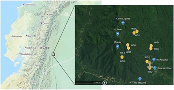
On site in Wisuí, 12 plots of 20 m × 20 m each were established, each covering an area of 400 m2 and numbered consecutively from WIS1 to WIS12 (Figure 1). Half of the plots were located in the lowlands at elevations between 658 and 688 m, while the other half was established along the mountain ridges of the Cordillera de Cutucú at elevations between 948 and 1055 m (Table 1). For each location, we recorded GPS coordinates, elevation (m), canopy height (m), inclination (°), exposition, total ground cover (%) and canopy cover (%). The sampling locations spread across an area of 3 km × 3.5 km (10.5 km2) with a geographical distance from 20 m to 3 km between them by air (Figure 1).

Figure 1. Location of the study area is in the lowlands of the Eastern Andes in Ecuador in the province Morona Santiago. The area is located at 675 m between the stream Kosutka and the mountain El Torre (1370 m) north of the river Macuma at S 02º 06.664' W 077º44.334'. Maps via OpenStreetMap (left, tiles courtesy of Andy Allan) and Google Earth (right, Landsat/Copernicus, Maxar Technologies).
Table 1. Geochemical characterisation for each of the n = 12 plots of the study area

Abbreviations: C, carbon; N, nitrogen; C:N, carbon to nitrogen ratio; Al, aluminium; Ca, calcium; Fe, iron; K, potassium; Mg, magnesium; Mn, manganese Na, sodium.
Inventory of fern communities
All fern species occurring within a plot were documented photographically, their life form was recorded (epiphytic, semi-epiphytic, terrestrial), whether they were sterile or fertile, rhizomes were characterised if present, and their abundance was recorded by counting all individuals within each plot. All plant samples were identified to species level and taxonomy was cross-checked at the herbarium in Quito (QCA) and against Hassler et al. (Reference Hassler, Bánki, Roskov, Döring, Ower, Vandepitte, Hobern, Remsen, Schalk, DeWalt, Keping, Miller, Orrell, Aalbu, Adlard, Adriaenssens, Aedo, Aescht, Akkari and Alexander2022). When existing plant material was sufficient, reference collections were made in quadruplicate. For this purpose, plant material was pressed in newspaper, disinfected with alcohol and stored in dark plastic bags. During the collection phase, plant material was regularly exported to be temporally deposited at the Ministry of Environment of the Province Morona-Santiago in Macas, and finally dried at the Universidad Católica in Quito. The dried duplicates were distributed to the herbaria of the Universidad Católica in Quito, Ecuador (QCA, including all unique samples), the Ministry of Environment of the Province Morona-Santiago in Macas, Ecuador (Ministerio del Ambiente, MAC), the State Museum of Natural History in Stuttgart, Germany (STU) and one partial collection was deposited at the NEES Institute for Biodiversity of Plants, University of Bonn, Germany (BONN). Of each separate collection, a sample of leaf tissue was preserved in silica gel for subsequent DNA extraction, sequencing and barcoding.
Determination of diversity
The sampling unit in all analyses is entire plots (400 m2) and all primary diversity measures refer to this spatial entity. In each plot, we measured the number of different species (s), their abundance, that is, how frequently they occur as determined by the number of individuals of a species per plot and their relative abundance, that is, the number of individuals of a species per plot (n) relative to the total number of individuals within such plot (N). Subsequently, we compare the species distributions amongst plots to unravel how diversity relates to edaphic and elevational parameters.
First, we define “species richness” as the actual number of different species present per plot (s). This is also known as “α-diversity” (Whittaker Reference Whittaker1972). To account for the fact that diversity depends not only on the number of species observed as such but also on how often these species occur in relation to the occurrence of the other species within the same plot, we calculated two complementary indices to describe “species diversity” normalising the number of species with the abundance of species.
We first calculated the Shannon index (H), which is an information statistic index, which means it assumes all species are represented in a sample and that they are randomly sampled:
 $${\rm{Shannon}}\ {\rm{index}}\,\left( H \right) = - \mathop \sum \limits_{i = 1}^s {p_i}\ln {p_i}$$
where (p) is the relative abundance, that is the proportion (n/N) of individuals of one particular species (n) divided by the total number of individuals (N) found in one plot, ln is the natural logarithm, Σ is the sum of the calculations and s is the number of species (Shannon Reference Shannon1948).
Secondly, we calculated the Simpson index (D), which is a dominance index giving more weight to common species. In this case, rare species with only a few representatives will not affect the diversity:
 $${\rm{Simpson}} \ {\rm{index}}\,\left( D \right)\; = \;1 - {{\sum {n_i}({n_i} - 1)} \over {N\left( {N - 1} \right)}},$$
where (n) is the number of individuals of one particular species and (N) is the total number of individuals found in one plot (Simpson Reference Simpson1949). The higher the number for this index, the higher the diversity of species.
Thirdly, we wanted to know how uniform species composition is, that is, if different species are represented by largely different or similar numbers of individuals. For this purpose, we calculated Pielou’s evenness index (J), which ranges between 0 and 1, where zero means no evenness and one means complete evenness, so all species occur with equal numbers of individuals.
 $${\rm{Pielou's}}\,{\rm{evenness}}\,{\rm{index:}}\left( J \right)\; = \;{{{\rm{Shannon\;index\;}}\left( {\rm{H}} \right){\rm{\;}}} \over {{\rm{Maximum\;Shannon\;index\;}}\left( {{H_{MAX}}} \right){\rm{\;}}}}.$$
where HMAX is the maximum possible value of the Shannon index H (if every species was equally likely) calculated as
 $${H_{Max}} = \mathop \sum \limits_{i = 1}^s {1 \over S}\ln {1 \over S} = {\rm{\;ln}}s$$
where (s) is the total number of species (Pielou Reference Pielou1966).
Diversity across scale
To compare species diversity amongst plots, we first calculated “β-diversity” as the number of species in all plots divided by the number of species in each individual plot (Whittaker Reference Whittaker1972). To then understand how diversity is affected by geographic distance, we first created a data frame with the Bray–Curtis coefficient (BC), which is a dissimilarity index with values between 0 and 1. The closer the value is to 0, the more the communities have in common:
 $${\rm{Bray {\hbox-} Curtis}}\ {\rm{dissimilarity}}\,{\rm{(BC)}} = 1 - {{2{C_{ab}}} \over {Sa + Sb}}$$
where (C) is the sum of the lowest number of species two communities a and b have in common, (Sa) is the total number of species found in community a and (Sb) is the total number of species found in community b (Bray & Curtis Reference Bray and Curtis1957). Then we created a similar data frame with the haversine distances between all pairs of plots and used the Mantel test for non-parametric Spearman correlations between the two distance matrices with 9999 permutations (Mantel Reference Mantel1967).
Soil analysis
In each plot (n = 12), approximately 150 g of the upper soil horizon were sampled for further analysis at the Institute for Ecology and Ecosystem Sciences at the University of Göttingen (Germany). Samples were first classified according to USDA Soil Taxonomy (Agriculture handbook 436, 1999). Then, soil pH was measured in water (H20) and in potassium chloride (KCl) and soil water content was determined on a subsample as mass fraction between fresh soil and the mass of soil dried at 105°C for 48 hours. Carbon and nitrogen contents were determined by combustion and thermal conductivity detection. Moreover, the effective exchangeable cation contents of aluminium (Al3+), calcium (Ca2+), iron (Fe2+), magnesium (Mg2+), manganese (Mn2+), potassium (K+) and sodium (Na+) were determined, where the sum of Ca2+, Mg2+, K+, and Na+ is the soils’ total base saturation and the sum of all exchangeable cations is the soils’ CEC, which equals its negative charge.
Statistical analysis
To test if species richness and diversity measures were different between the two elevational ranges (658–688 m) and (948–1055 m), we used Welch’s t-test (Welch Reference Welch1947). Partial least square (pls) regression was applied to identify which geochemical parameters drive diversity, defined as species richness (α-diversity) and via the two diversity indices after Shannon and Simpson, respectively. In each pls model, the number of predictors was first reduced via ordination and then a subset of latent variables was extracted to predict the response using regression. The pls models were fitted with the kernel algorithm, validated by inspecting the root mean square error of prediction and cross-validated using six leave-one-out segments (Liland et al. Reference Liland, Mevik and Wehrens2021, Mevic & Wehrens Reference Mevic and Wehrens2021). All statistical analysis was carried out using R 4.0.5 (R Core Team, 2021) with the additional packages “geosphere” (Hijmans Reference Hijmans2022), “ggplot2” (Wickham Reference Wickham2016), “ggpubr” (Kassambara Reference Kassambara2020), “pls” (Liland et al. Reference Liland, Mevik and Wehrens2021) and “vegan” (Oksanen et al. Reference Oksanen, Simpson, Blanchet, Kindt, Legendre, Minchin, O’Hara, Solymos, Stevens, Szoecs, Wagner, Barbour, Bedward, Bolker, Borcard, Carvalho, Chirico, De Caceres, Durand, Antoniazi Evangelista, FitzJohn, Friendly, Furneaux, Hannigan, Hill, Lahti, McGlinn, Ouellette, Ribeiro Cunha, Smith, Stier, Ter Braak and Weedon2022).
Results
Fern diversity
In total, 213 primary specimen samples were collected. They comprised 133 different fern species, of which 116 occurred in the plots presented here, while the additional species were collected at mountain summits, between plots and along the river Kosutka (Figure 1, supplementary data 1). The identified species belong to 49 genera of 22 families and stand representative for 3376 individual ferns, of which 795 grew terrestrially while 1925 grew epiphytically. An additional group of 656 individuals was found partly climbing on roots, wood or rocks or in other semi-epiphytic habitats. We identified two highly cosmopolitan species, Campyloneurum repens (Aubl.) C. Presl and Nephrolepis rivularis (Vahl) Mett., each of which occurred in 7 out of the 12 plots. The overall most cosmopolitan genera were Polybotrya and Microgramma, while the genera with the largest populations were Dennstaedtia, Didymochlaena and Campyloneurum. The most abundant family was Polypodiaceae representing 39 individuals (18% of all specimen).
Environmental parameters
Most soils were classified in-between Entisoles and Inceptisols or ranked as Alfisol or Ultisols (Table 1). Environmental parameters followed the trends predicted from the literature to distinguish the two elevations. For example, canopy height and total ground cover were higher in lower elevations, while inclination was higher in higher elevations. Soil pH, carbon and nitrogen contents and base saturation were also higher in lower elevations. Most soils were acidic to moderately acidic, with pH (in water) between 4 and 5. In three plots (WIS2, WIS7, WIS11), soil pH was less acidic (>5), with the highest pH measured for the soil of WIS 2 (pH = 6.82 in water). Carbon contents were between 5% and 15%, nitrogen contents between 0.5% and 0.9% and most soils had a C:N ratio around 12. The sum of exchangeable cations was also higher in lower elevations compared to high elevations. Notably here is the elevated calcium, potassium and magnesium in WIS11 and elevated sodium in the soils of WIS2, WIS12 and WIS1. Finally, elevated aluminium and iron concentrations separated the two high elevational sites WIS9 and WIS10 from the other plots (P = 0.001) and manganese was overall more abundant in the higher elevations as compared to the lower elevations (P = 0.04).
Fern diversity and elevation
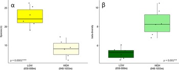
We found a strong relationship (P = 0.0001) between elevation and species diversity when assessing diversity as count data of species occurrences (Figure 2). The simplest measure of species richness, that is the number of species per plot (α-diversity), was higher in lower elevations as compared to the higher elevational range (Figure 2 left), while the differentiation amongst plots (β-diversity) increased with increasing elevation (Figure 2 right).

Figure 2. Fern α-diversity (left) and β-diversity (right) at two elevation ranges (658–688 m and 948–1055 m) in a low-montane Amazon rainforest. Results of Welch’s t-test comparing means of species richness and beta diversity, respectively, are given in each plot with asterisks indicating the significance level at <0.001 ‘***’ and ≤0.01 ‘**’.
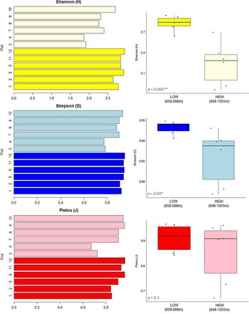
When taking the complexity of community composition into account, that is, the frequency of occurrences of individuals of a single species in relation to overall species abundance, these general trends were supported by higher Shannon and Simpsons indices in the lower elevational range (Figure 3). There was no significant difference in species evenness (Pielou index) between elevations (P = 0.3). However, for the two high elevational plots WIS3 and WIS4, we found lower diversity indices and also less evenness in species composition.

Figure 3. Shannon (H), Simpson (D) and Pielou (J) diversity indices for the 12 plots studied. In lighter colors, the plots are from the higher elevational range (948–1055 m), and in dark, the plots are from the lower elevational range (658–688 m). Consistently lower species diversity (H, D) and evenness (J) in the higher elevational plots, notably plots WIS3 and WIS4.
To determine the drivers of diversity, we performed pls modelling for α-diversity and the two diversity indices (Table 2). In all cases, the first two components explained over 90% of variance (93.4%, 93.21% and 92.32%, respectively). Elevation was consistently inversely correlated with the respective diversity measures, while exposition was mostly positively correlated with diversity. CEC was the second strongest vector for all three diversity measures, mostly driven by aluminium and calcium concentrations.
Table 2. Results of ordination and least square regression (pls) explaining species richness (α-diversity) and diversity (Shannon and Simpson indices) at plot level based on the geochemical data. Only the loadings of the first two components are shown. They explain >90% variance in each model

Geographic distance and dissimilarity
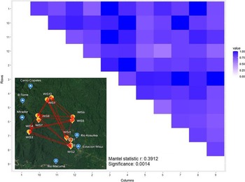
We used the Bray–Curtis dissimilarity (BC) to quantify diversification between plant communities amongst all pairs of the 12 plots as a function of geographic distance using Mantel test (Figure 4). Overall, the dissimilarity between plots increased significantly with increasing geographic distance between them (r = 0.39, P = 0.001). Hence, the farther two plots are away from each other, the greater the difference in community composition.

Figure 4. Heatmap shows Bray–Curtis dissimilarities between all pairs of plots (the closer a value is to 0, the more the communities have in common) and map in bottom left corner shows the location of the 12 plots with arrows indicating haversine distance measure. Result of Mantel test investigating the correlation between diversity and geographic distance was significant at P < 0.01 with r = 0.39 with geographic distance being proportional to diversification between plots.
Discussion
In terms of species richness (α-diversity), the empirical data of this study support our first hypothesis (H1), which stated that diversity would decrease with elevation (P = 0.0002; Figure 2). This pattern was confirmed when taking species abundance into account, as two diversity indices also decreased with elevation (Figure 3). The second hypothesis (H2), which stated that diversity would be unaffected by soil nutrient richness, had to be rejected as CEC was amongst the main drivers of the observed diversity patterns (Table 2) and some plots were notably characterised through moderately to strongly elevated aluminium concentrations in the soil (WIS3, WIS4, WIS9, WIS10; Table 1). The third hypothesis was confirmatory, stating that similarity between communities would decrease with increasing geographic distance between sampling sites and was strongly supported (r = 0.39, P = 0.001; Figure 4).
Clear link between diversity and elevation
In the long and eventful history of describing species assemblages along elevational gradients, Alexander von Humboldt was one of the first to describe a hump-shaped pattern of species richness on mountains, which increases towards mid-elevations and then decreases again towards the summit (Humboldt Reference Humboldt1860). This pattern was confirmed in many subsequent studies (reviewed in Hawkins et al. Reference Hawkins, Field, Cornell, Currie, Guégan, Kaufman, Kerr, Mittelbach, Oberdorff, O’Brien, Porter and Turner2003), including for ferns and lycophytes in the Himalayas (Bhattarai & Vetaas Reference Bhattarai and Vetaas2003), Africa (Aldasoro et al. Reference Aldasoro, Cabezas and Aedo2004), Bolivia (Kessler Reference Kessler2001) and Costa Rica (Kluge et al. Reference Kluge, Kessler and Dunn2006). The data presented here describes a low-elevational mountain ridge, but the higher sampling sites are relatively close to mountain summits El Torre at 1370 m and Cerro Copales at 996.5 m. The mountain slopes studied here therefore share some geological features with higher elevational mountain slopes, like exposure and also at times north-eastern trade winds. Hence, the observed decline of biodiversity with elevation is comparable to the decline observed on longer gradients above the mid-elevation hump and towards the summit.
Biological niche separation to boost biodiversity
The higher diversity in the lower elevational range may also be explained by greater canopy cover and niche separation within the denser forest, which favours species diversity through habitat and niche differentiation (Suissa et al. Reference Suissa, Sundue and Testo2021, Wright Reference Wright2002). Niche separation was also expressed in the variation of fern life form, for example, the ratio between terrestrial and epiphytic ferns amongst plots, as well as in plant morphology. The strictly terrestrial habitat was mostly dominated by larger plants, including tree ferns such as different Cyathea species, frequently found with compound or dissected fronds. Meanwhile, the semi-epiphytic and epiphytic habitats on tree trunks and branches were occupied by smaller fern species, of generally single leaflets, present in large populations (e.g. Didymoglossum ovale, several hundred in WIS2). This habitat differentiation is common in tropical rain forests and contributes to the high species diversity (Jones et al. Reference Jones, Szyska and Kessler2011, Watkins & Cardelús Reference Watkins and Cardelús2009).
Soil heterogeneity enhances community dissimilarity across geographic distance
Even though our sampling was restricted to a relatively small geographical scale, we clearly observed that the farther away plots were geographically, the greater was the difference in their community composition (Figure 2 right, Figure 4). This well-described fact is usually explained by dispersal limitation and/or changes in climatic conditions (Colwell et al. Reference Colwell, Brehm, Cardelús, Gilman and Longino2008, Rehm & Feeley Reference Rehm and Feeley2015) and may in this study be amplified by effects of topography and relief, which increases the actual distance between two sides beyond the spherical distance. Especially plots WIS3 and WIS4 were separated from the other plots in terms of their fern communities, but also geographically, as they are physically separated from the other plots by a steep hillside furrow (Figure 1). The plots also showed lower evenness, which was likely driven by few species occurring in particular high densities, namely Danaea cf. bicolour (Marattiaceae) in WIS3 and Lindsaea schomburgkii (Dennstaedtiaceae), Cochlidium serrulatum (Grammitidaceae) and Didymoglossum hymenoides (Hymenophyllaceae) in WIS4.
Overall, soil formation and topography play a major role in shaping the study area, which is located on the eastern side of the foothills of the posterior ascended Cutucú uplift of the Andean mountains. The major uplift of the Central Andes that passes through the country has been dated back to the middle Miocene when today’s two-ridged shape of the mountain chain arose (Coltorti & Ollier Reference Coltorti and Ollier2000). A prominent event in geological soil formation was the rise of the still active volcano Sangay (5230 m) located 60 km west to the investigated sites at Wisuí. This led to partially exposed Palaeozoic to Tertiary basements partially covered by Jurassic to Cretaceous sedimentary and volcanic rocks, including sandstone and volcanic basaltic and andesitic lavas (Balseca et al. Reference Balseca, Ferrari, Pasquare and Tibaldi1993, Ruiz et al. Reference Ruiz, Seaward and Winkler2007, White et al. Reference White, Skopec, Ramirez, Rodas and Bonilla1995). This sedimentary sequence followed the individual topography of the Andes down to the lowlands. Consequently, the soil presents highly heterogenic patterns of erosion, sedimentation and exposed preserved older rocks, which built a complex network of rather distinct soils along the Ecuadorian landscape with the clay containing layers typically formed by calcite (CaCO3) or dolomite (CaMg(CO3)2) (Lathwell & Grove Reference Lathwell and Grove1986), explaining the increased CEC of magnesium (Mg2+) but most notably calcium (Ca2+) in the here studied soils (Table 1). This diversity of soils is likely contributing to the high plant diversity (Tuomisto et al. Reference Tuomisto, Zuquim and Cárdenas2014, da Costa et al. Reference da Costa, Arnan, de Paiva Farias and Leão Barros2019, Moulatlet et al. Reference Moulatlet, Zuquim and Tuomisto2019).
Soil acidification and cation exchanges – between nutrient enrichment and metal toxicity
The high water inputs from precipitation in the Amazon basin can increase the elution of nutrients from soil by leaching (Richter & Babbar Reference Richter and Babbar1991, Stallard & Edmond Reference Stallard and Edmond1983), which can lead to soil acidification when extended amounts of bases are swamped out. This manifests in low soil pH, for example, the case for the plots on Cerro Copales (WIS9 and WIS10). Due to the acidic milieu, the light metal aluminium switches from the silicate lattices of the subsoil horizon and the positions of the exchangers are occupied by hydronium (H3O+). Aluminium becomes the predominant ion of the exchange complex. The clay fraction of these soils is dominated by kaolinite (Al2Si2O5(OH)4) and presumably contains smaller amounts of goethite (HFeO2) and haematite (Fe2O3). Therefore, only in these samples iron (Fe2+) could be detected (Table 1). Environmental factors like warming, weathering and nitrogen deposition can all trigger the exchanges of cations on soil mineral binding sites (Cusack et al. Reference Cusack, Macy and McDowell2016) and thus liberate currently limiting nutrients like iron, but future studies could also monitor closely the release of potentially toxic cations such as aluminium (Al3+). If these cations are released in excess in the future, the consequences for plant community composition and species diversity could be severe.
Conclusion
Fern species richness and diversity were overall best explained by elevation and soil CEC, notably aluminium and calcium concentrations. Further monitoring ferns could therefore help to better understand and predict how environmental change may impact biodiversity, with a particular focus on threads potentially arising from elements being released in excess from tropical soils through modified soil CEC.
Supplementary material
To view supplementary material for this article, please visit https://doi.org/10.1017/S0266467423000081
Acknowledgments
We are grateful to the Cotán family in Wisuí for their warm welcome and for safely guiding us through the jungle (yuminsajme). We also thank Victor León in Macas for safekeeping our fern samples during the collections and the team of the herbarium in Quito for all their help with drying and identifying fern species and recording the samples to the collection. We thank Dietrich Hertel and his team in Göttingen for their help with soil analysis. The financial support of the DFG (grants LE1826/4 and QU153/7) is greatly acknowledged. Research permits (No. 03-2012-Investigación-B-DPMS/MAE) were kindly issued by the Ministerio del Ambiente, Dirección Provincial del Morona-Santiago.
Financial support
Deutsche Forschungsgesellschaft (DFG) grants LE1826/4 and QU153/7.
Conflicts of interest
The authors have no competing interests to declare.


 Open access