The Verlinde traces for $SU_{X}(2,\xi )$ and blow-ups

Abstract

Given a compact Riemann surface X of genus at least 2 with automorphism group G, we provide formulae that enable us to compute traces of automorphisms of X on the space of global sections of G-linearized line bundles defined on certain blow-ups of projective spaces along the curve X. The method is an adaptation of one used by Thaddeus to compute the dimensions of those spaces. In particular, we can compute the traces of automorphisms of X on the Verlinde spaces corresponding to the moduli space $SU_{X}(2,\xi )$ when $\xi$ is a line bundle G-linearized of suitable degree.

1 Introduction

Let X be a complex, irreducible, smooth, projective curve of genus at least 2 and automorphism group $G=Aut(X)$. Let $\xi$ be a $G-$linearized line bundle over X.

By the Verlinde traces, we refer to the traces of automorphisms of X on the space , where $SU_{X}(r,\xi )$ is the moduli space of semi-stable rank r vector bundles with determinant $\xi$ and where is the determinantal line bundle of $SU_{X}(r,\xi )$. In this work, we address the problem of computing the Verlinde traces for the case $r=2$ and we give a way to compute them which is alternative to the approach of J. E. Andersen for case of the trace in [2] pg. 3 ( in our case).

Our method and result will be explained in the paragraphs below. Before that, we would like to mention a few things related to this problem. As the reader may be aware the case of the Verlinde traces for the identity of G is already solved. A formula for dim was conjectured by E. Verlinde [34] and there are many proofs of it(see for instance the following works concerning this case [7, 8, 12, 15, 17, 28, 31,32,33, 35] and [36]). The action of non-trivial automorphism groups G on the Verlinde spaces had already been considered in the work of Dolgachev ([13] in his proof of Cor. 6.3), in the work of the first author [23] (see Tables 1–4 there) where some Verlinde traces are computed for the cases , $n=1$ and arbitrary rank r by computing them on and later in the work of Andersen [2] the Verlinde traces correspond to the traces which we will briefly refer to at the end of this introduction.

As there are automorphisms of $SU_{X}(r,\xi )$ that are not induced by G (for a description $Aut(SU_{X}(r,\xi ))$ and related results see [9, 20, 21]) we should also mention that the action of torsion elements of the Jacobian of X acting on the Verlinde spaces of some moduli spaces of vector bundles had also been considered in the works [6, 27, 29]. Explicit formulae for the corresponding Verlinde traces are provided in [6] and [29].

Coming back to our problem, in the rank 2 case, we followed the method used by Thaddeus to derive the Verlinde formula in [32]. We shall see that his method can be extended to compute the Verlinde traces (see formula (4.9) and Sect. 5) by just replacing the use of the Riemann–Roch Theorem for the use of the Atiyah–Singer Holomorphic Lefschetz Theorem (see Sect. 3) and in this work, we derive some formulae (Theorem 8.1 ) required to apply the Holomorphic Lefschetz Theorem in Thaddeus’ method.

Let $K_{X}$ be the canonical line bundle of X. Suppose that $K_{X}\xi$ is very ample. Let $X\hookrightarrow \mathbb {P}^{N}$ be the embedding defined by the complete linear system $\mid K_{X}\xi \mid$. Let $\pi :\widetilde{\mathbb {P}^{N}_{X}}\mapsto \mathbb {P}^{N}$ be the blow-up of $\mathbb {P}^{N}$ with center X and let E be the corresponding exceptional divisor. The Picard group of $\widetilde{\mathbb {P}^{N}_{X}}$ is generated by and the hyperplane line bundle . For integers m, n let and let . Let $\xi$ have degree d. Thaddeus shows that for $d>2g_{X}-2$ there is a natural isomorphism

(1.1)

Under some mild conditions on m, n he finds a formula for the dimension of $V_{m,n}$ (see Theorem 4.1 below). The cases not covered by those conditions can be dealt with easily.

Now, when we assume that $\xi$ is G-linearized it induces an action of G on $\mathbb {P}^{N}$ and on the blow-up $\widetilde{\mathbb {P}^{N}_{X}}$ such that the embedding $X\hookrightarrow \mathbb {P}^{N}$ and the blow-up map $\pi$ are G-equivariant. The line bundles can be equipped with a linearization induced by that of $\xi$. That is because comes equipped with a linearization induced by that of $\xi$; also since E is a G-invariant divisor admits a linearization of G with trivial action on , and since we can see that this linearization is unique(with trivial action on ) because there is a bijection between the G-linearizations of and the G-invariant divisors linearly equivalent to E by G-invariant rational functions (see [13] Prop. 2.1 and [14] Ex. 7.4). So one can consider the problem of computing the traces of elements of G on the spaces $V_{m,n}$ (Thaddeus traces). As we will see in Sect. 4, the formula for $dim V_{m,n}$ is a linear combination of Euler Characteristics of sheaves $B_{i,m,n}$ defined over symmetric products $S^{i}X$ of the curve (see Theorem 4.1 below) and these sheaves are naturally G-linearized. By tracking back the proof of Theorem 4.1 one notice that the homomorphisms between the cohomology groups involved are G-equivariant and that the trace of an element $h\in G$ on $V_{m,n}$ is in fact obtained by replacing the Euler characteristics of the sheaves $B_{i,m,n}$ by their corresponding Lefschetz numbers $N_{i}(h)=L(h,B_{i,m,n})$ (see formula (4.9) below and Sect. 5 for its proof). These Lefschetz numbers $L(h,B_{i,m,n})$ can be computed using the Holomorphic Lefschetz Theorem (see Sect. 3, Theorem 3.1 and formula (3.6)) because the sheaves $B_{i,m,n}$ are defined on smooth varieties. To do that we need to know for each component Z of the fixed point set the following data: the generalized Chern Character $\text {ch}_{h}(i^{*}_{Z}B_{i,m,n})$ (see (3.1)), the stable characteristic classes $U(N_{Z/S^{i}X}(\nu ^{j}))$ of the normal bundle $N_{Z/S^{i}X}$ (see (3.2)), the Todd class $\text {Td}(T_{Z})$ of the tangent bundle $T_{Z}$ and $\text {det}(Id-h_{\mid }{N^{\vee }_{Z/S^{i}X}})$ (see Theorem 3.1). In this way by equation (3.6), the solution of the problem of computing $N_{i}(h)=L(h,B_{i,m,n})$ is reduced to the calculation of the following intersection numbers, namely, the contributions

(1.2)

of each component $Z\subseteq {(S^{i}X)}^{h}$ of the fixed point set of h.

As we pointed out earlier, the main goal of this paper (Theorem 8.1) is the calculation of the generalized Chern Character $\text {ch}_{h}(i^{*}_{Z}B_{i,m,n})$. The other data required to apply (1.2) have been dealt with in the works [23](Prop. 3.2) and [24] (Theorem 2.3). However, in Sect. 7, we present a generalization of the formula for the stable characteristic classes $U(N_{Z/S^{i}X}(\nu ^{j}))$ that was given in [24]. The Theorem 6.1 is required for the proof of Theorem 8.1 and part of its proof is modelled on the proof of Proposition 2.1 in [24]. At the end of the paper we illustrate the use of formula (4.9), when X is a hyperelliptic curve of genus 2, by computing the Verlinde traces corresponding to the hyperelliptic involution.

The problem of computing Verlinde traces may be considered interesting in its own right and following the work of Thaddeus on moduli of pairs there have been various constructions of series flips using moduli of pairs, triplets, that one should expect to be able to use to compute Verlinde traces on moduli spaces other than $SU_{X}(2,\xi )$. Some of our motivations are to determine the isotypic decomposition of the Verlinde spaces to study the varieties defined as the zero locus of the invariant submodules in, for instance, ; to study the Cox Ring of Blow-ups( in this case with the Thaddeus traces). Also, as it can be seen from the work of Andersen, Verlinde traces are used to compute invariants of 3-Manifolds, namely, the Witten-Reshetikhin-Turaev invariants of finite order mapping tori . Andersen considers moduli spaces of semi-stable -bundles on curves and by applying directly the Lefschetz–Riemann–Roch Theorem for singular varieties (see [5]) to the determinantal line bundle of the moduli spaces he obtained an expression for the traces because the higher cohomologies of the determinantal line bundle vanish. The formula is given by the equation 8.1 or Theorem 1.3 in [2] up to the correction factor $Det(f)^{-\frac{1}{2}\zeta }$, and depends on data coming from the components of the fixed point set. The moduli spaces correspond to the case and a description of the components of fixed point set for this case is given in Theorem 6.10 of [2] (see also Theorem 3.4 of [1]). The contribution of the smooth components to the traces is also determined in his work. In the rank 2 case, the advantage of our method is that one does not have to deal with singular components of fixed points and one can compute the Verlinde traces if one knows the action of the automorphism on the tangent spaces of the fixed points in the curve.

Some results of this work are based on results of the Ph.D Thesis of the second author [30].

2 Notation

Let p be a positive integer and let $\nu =\exp (2i\pi /p)$. Given a finite cyclic group $H=\langle h \rangle$ of order p acting trivially on a variety Z and given an H-linearized vector bundle F on Z there is a decomposition into eigenbundles

$$\begin{aligned} F=\bigoplus _{j=0}^{p-1} F(\nu ^j), \end{aligned}$$

that is, $F(\nu ^j)$ is the sub-bundle of F where the action of h on the fibres is multiplication by $\nu ^j$. Most of the times we will say that F is h-linearized.

For a divisor D on a variety W we write (or just ) to denote corresponding line-bundle of D. If F is a sheaf on W we usually write F(D) rather than . Usually $F^{n}=F^{\otimes n}$, also if K is another sheaf some times we could write $KF= K\otimes F$. If ${\xi }$ is a sheaf on W and $\xi '$ is a sheaf on X we use the notation $\xi \boxtimes \xi '=\pi ^{*}_{W}\xi \otimes \pi ^{*}_{X}\xi '$ on the product $W\times X$, where $\pi _{W}$ and $\pi _{X}$ are the natural projections and if G is a sheaf on $W\times X$ we sometimes write $\xi G=\pi _{W}^{*}\xi \otimes G$ (or $\xi (D)$ instead of $\xi G$ if with $D\subset W\times X$ is a divisor).

If $i:\Delta \hookrightarrow W$ is the inclusion of a subvariety of W then is the pull-back $i^{*}F$ for any sheaf F on W and if $\Delta$ is a divisor of W then we denote . If F is locally free then $F^{\vee }$ is the dual sheaf and we also denote by F the vector bundle whose sheaves of sections is F. If $x\in W$ then $F_{x}$ is the fibre of F at the point x. For a vector bundle F over X we denote by $\pi :\mathbb {P}(F)\rightarrow X$ the projective bundle of one dimensional subspaces of F thus where $Sym(E)=\oplus _{m} S^{m}E$ is the symmetric algebra of a locally free sheaf E over X. The exponential function $exp(x)=\sum _{n=0}^{\infty }x^{n}/n!$ is also be represented by $e^{x}$ and in some formulae we mixed both notations.

3 The Holomorphic Lefschetz theorem

Consider a finite cyclic group $H=\langle h \rangle$ of order $p\ge 1$.

Suppose that H is acting trivially on a variety Z and also consider an h-linearized vector bundle F on Z. The generalized Chern character of F is given by

$$\begin{aligned} ch_{h}(F)=\sum _{j=0}^{p-1}\nu ^{j}ch[F(\nu ^{j})], \end{aligned}$$

(3.1)

where $ch[F(\nu ^{j})]$ is the Chern character of the eigenbundle $F(\nu ^{j})$. For each vector bundle $F(\nu ^{j})$ with $\nu ^{j}\not =1$ define the stable characteristic class $U(\!F(\nu ^{j})\!)$ as

$$\begin{aligned} U(F(\nu ^{j}))=\prod _{i=1}^{r_{j}}\left( \frac{1-\frac{e^{-x_{i}}}{\nu ^{j}}}{1-\frac{1}{\nu ^{j}}}\right) ^{-1}, \end{aligned}$$

(3.2)

where $r_{j}$ is the rank $F(\nu ^{j})$ and the $x_{i}$’s are the Chern roots of $F(\nu ^{j})$.

We now make some observations about fixed point sets of h acting on non singular Varieties (see pg. 537 in [3] and Lemma 4.1 in [16]). Let X be an irreducible, non-singular complex algebraic variety on which h acts as an automorphism of X. Let $X^{h}$ denote the set of fixed points of h in X. One has that $X^{h}$ is non-singular and if $x\in X^{h}$ then as an analytic variety $X^{h}$ is (in a neighbourhood of x) the image, under a suitable equivariant exponential map, of the eigenspace $T_{X,x}(\nu ^{0})$ of the tangent space $T_{X,x}$ to X at x. As $T_{X^{h},x}=T_{X,x}(\nu ^{0})$ one has that the linear transformation $h_{\mid } N_{X^{h}/X,x}$ induced by h on the normal space $N_{X^{h}/X,x}$ to $X^{h}$ at x has no eigenvalue $\nu ^0$ and therefore

$$\begin{aligned} \det (Id-h\mid N_{X^{h}/X,x})\not =0. \end{aligned}$$

(3.3)

One also notice from what was said above that $X^{h}$ is locally irreducible so a point $x\in X^{h}$ belongs to a unique irreducible component of $X^{h}$ and so

$$\begin{aligned} X^{h}=\coprod _{Z\in CX^{h}} Z, \end{aligned}$$

(3.4)

where $CX^{h}$ is the set of irreducible components of $X^{h}$.

Let $i_{X^{h}}:X^{h}\hookrightarrow X$ the inclusion $X^{h}\subseteq X$. Let E be an h-linearized vector bundle on X. The Lefschetz number L(h, E) (sometimes written L(h, X, E)) of h on E is

$$\begin{aligned} L(h,E)= \sum _{i}(-1)^{i}trz\ h|H^{i}(X,E) \end{aligned}$$

and can be computed by the Holomorphic Lefschetz Theorem:

Theorem 3.1

(Atiyah–Singer, Theorem 4.6, pg. 566, [4])

(3.5)

where ${\text {det}(Id-h_{\mid }{N^{\vee }_{X^{h}/X}})}$ assigns to the component of $x\in X^{h}$ the value of ${\text {det}(Id-h_{\mid }{N^{\vee }_{X^{h}/X,x}})}.$ Also, $U(N_{X^{h}/X}(\nu ^{j}))$ is the stable characteristic class of $N_{X^{h}/X}(\nu ^{j})$, ch$_{h}(i^{*}_{X^{h}}E)$ is the generalized Chern character of the pull-back $i^{*}_{X^{h}}E$ of E to $X^{h}$ and $\text {Td}(T_{X^{h}})$ is the Todd class of the tangent sheaf $T_{X^{h}}$ of $X^{h}$.

On the right-hand side of (3.5), one is evaluating a cohomology class $u\in H^{*}(X^{h},{\mathbb {C}})$ (here u is the integrand). By (3.4) on has that

$$\begin{aligned} H^{*}(X^{h},{\mathbb {C}})=\bigoplus _{Z\in CX^{h}} H^{*}(Z,{\mathbb {C}}) \end{aligned}$$

and then the evaluation of u is the sum of the evaluations of the components $u_{Z}\in H^{*}(Z,{\mathbb {C}})$ of u, that is,

(3.6)

A particular case of Theorem 3.1 is the Atiyah-Bott formula also known as the Woods Hole Fixed Point Theorem which is obtained when $X^{h}$ is a finite set:

$$\begin{aligned} L(h,E)=\sum _{x\in X^{h}}\frac{trz \ h|E_{x}}{det(Id-h|T^{\vee }_{X,x})}, \end{aligned}$$

(3.7)

where $trz \ h|E_{x}$ is the trace of $h|E_{x}$ (see [10] pgs. 631 and 121).

4 The trace formula

From now on what follows X will denote the curve considered in the introduction, that is, a complex, irreducible, smooth curve of genus $g\ge 2$ embedded in $\mathbb {P}^{N}=\mathbb {P}H^{1}(\xi ^{-1})$ via the linear system $|K_{X}\xi |$, where $\xi$ is a line bundle on X of degree d.

Let $\pi _{S^{i}X} : X\times S^{i}X\mapsto S^{i}X$ and $\pi _{X}:X\times S^{i}X\mapsto X$ be the natural projections. Let $\Delta _{i}\subset X\times S^{i}X$ be the universal divisor and let $j'$ denote its inclusion into $X\times S^{i}X$. Consider the Thaddeus bundles

(4.1)

and

(4.2)

One has that $W^{-}_{i}$ is a vector bundle of rank i and that if $-d+2i < 0$ then $W^{+}_{i}$ is a vector bundle of rank $d+g-1-2i$.

Define

(4.3)

where $(\pi _{S^{i}X})_{!}:K(X\times S^{i}X)\rightarrow K(S^{i}X)$ is the direct image homomorphism between Grothendieck groups given by

$$\begin{aligned} (\pi _{S^{i}X})_{!}({\mathscr {F}}) =\sum _{i}(-1)^{i}{R^{i}_{\pi _{S^{i}X}*}} ({\mathscr {F}}) \end{aligned}$$

(4.4)

for a coherent sheaf ${\mathscr {F}}$ over $X\times S^{i}X$ (See [19] pg. 436). Also, $\det :K(S^{i}X)\rightarrow Pic(S^{i}X)$ is the group homomorphism between the additive group $K(S^{i}X)$ and the multiplicative group $Pic(S^{i}X)$ given by

(4.5)

where $a_{1},\cdots , a_{m}\in {\mathbb {Z}}$, the are coherent sheaves and is the usual determinant of coherent sheaves defined by means of a locally free resolution of .

Let $U_{i}\rightarrow S^{i}X$ be the bundle

$$\begin{aligned} U_{i}=W_{i}^{-}\oplus (W_{i}^{+})^{\vee }. \end{aligned}$$

(4.6)

Let $q_{i}=n-(i-1)m$. For $i>0$ consider the Euler characteristic

$$\begin{aligned} N_{i}=\chi (S^{i}X,B_{i,m,n}), \end{aligned}$$

(4.7)

where

$$\begin{aligned} B_{i,m,n}=L_{i}^{m}\otimes \wedge ^{i}W_{i}^{-}\otimes S^{q_{i}-i}U_{i}. \end{aligned}$$

(4.8)

For $i=0$ we define $B_{0,m,n}=S^{m+n}H^{0}(X,K_{X}\xi )$ and $N_{0}=dim B_{0,m,n}$. It is a convention that $B_{i,m,n}=0$ when $q_{i}-i<0$.

Theorem 4.1

(See (6.9) in [32]) Let $m,n\ge 0$ and suppose that $m(d-2)-2n > -d+2g-2$. Then

$$\begin{aligned} dim V_{m,n}=\sum _{i=0}^{\infty }(-1)^{i}N_{i}=\sum _{i=0}^{w}(-1)^{i}N_{i}, \end{aligned}$$

where $w=[(d-1)/2]$.

Under our hypothesis (namely, those of Theorem 4.1 together with the one that X has automorphism group G and that $\xi$ is G-linearized so that line bundles are G-linearized) one has that for any $h\in G$ (see Sect. 5)

$$\begin{aligned} Trace( h_{\mid _{ V_{m,n}}} ) =\sum _{i=0}^{\infty }(-1)^{i}N_{i}(h)=\sum _{i=0}^{w}(-1)^{i}N_{i}(h), \end{aligned}$$

(4.9)

where $N_{i}(h)$ stands for the Lefschetz number

$$\begin{aligned} L(h,B_{i,m,n} )=\sum _{j=0}^{i} (-1)^{j} Trace(h_{\mid _{}}{{ H^j(S^{i}X,B_{i,m,n}) }}), \end{aligned}$$

(4.10)

and for $i=0$,

$$\begin{aligned} N_{0}(h)=Trace(h_{\mid _{}}B_{0,m,n})=\underset{t^{m+n}}{coef}\left[ \frac{1}{\det (I-t\cdot h_{\mid _{}} H^{0}(X,K_{X}\xi ))}\right] . \end{aligned}$$

(4.11)

The far right-hand side of (4.11) follows from the proof of Molien’s Theorem 1.10 in [25]. So the Lefschetz numbers $N_{i}(h)$, $i>0$, can be computed by means of the Holomorphic Lefschetz Theorem if one (see formula (3.6)) can determine the contribution

of each component $Z\subseteq {(S^{i}X)}^{h}$ of the fixed point set. It will be explained in Sect. 6 that the components Z of ${(S^{i}X)}^{h}$ are parametrized by certain set of h-invariant divisors D on the curve X so in the subsequent sections we will write $Z_{D}$ rather than just Z because although components associated to distinct divisors may be isomorphic the data associated to them may not be the same. So far, the main obstruction to compute $C_{i,Z}(h)$ is the generalized Chern character $\text {ch}_{h}(i^{*}_{Z}B_{i,m,n})$ and it will be determined in Sect. 8. In Sect. 7, Theorem 7.1 we present a new formula for the stable characteristic classes $\text {U}(N_{Z/{S^{i}X}}(\nu ^{j}))$ and in (7.5) one for ${\text {det}(Id-h_{\mid }{N^{\vee }_{Z/{S^{i}X}}})}.$ The Todd class of a component is given in formula (6.8).

5 The proof of Thaddeus

Here we shall derive formula (4.9) so we are assuming that a finite group G is acting on the curve X and that $\xi$ is a G-linearized line bundle of degree d. Recall also that $K_{X}\xi$ is very ample and X is embedded into $\mathbb {P}H^{1}(X,\xi ^{-1})$ by the complete linear system $\mid K_{X}\xi \mid$. We should remark that $\xi$ plays the role of the line bundle $\Lambda$ considered in [32]. Thaddeus’ proof of Theorem 4.1 uses 4 results ((6.2),(6.6),(6.7) and (6.8) in [32] ) which we will state here in terms of Lefschetz numbers ( see Lemmas 5.1–5.4 below), their proofs follow from those of Thaddeus so we are essentially sketching his proof.

We start by introducing some notation related to the main tool which is a series of flips, depicted in the diagram (5.1) below, that connects the space $\mathbb {P}H^{1}(X,\xi ^{-1})$ and the moduli space $SU_{X}(2,\xi )$.

The spaces $M_{i}$ are constructed as moduli spaces of $\sigma _{i}$-stable pairs where is a rank 2 vector bundle on the curve X such that , and $\sigma _{i}\in (max(0,d/2-i-1),d/2-i)$ (for the definition of the stability condition see (1.1) in [32]). The space $M_{1}$ is $\widetilde{\mathbb {P}}^{N}_{X}$ the blow-up of $\mathbb {P}H^{1}(X,\xi ^{-1})$ along X embedded via $\mid K_{X}\xi \mid$. When $i=w=[(d-1)/2]$ the map $M_{w}\mapsto N$ has fibre over a stable bundle and it is surjective if $d>2g-2$. All the spaces $M_{i}$ turn out to be smooth, integral, rational projective varieties of dimension $d+g-1$ and for $i>0$ there is a birational map $M_{i}\leftrightarrow M_{1}$ which is an isomorphism except on closed sets of codimension at least 2. In fact there are embeddings $\mathbb {P}W_{i}^{+}\hookrightarrow M_{i}$ and $\mathbb {P}W_{i}^{-}\hookrightarrow M_{i-1}$, for $0<i\le (d-1)/2$, whose images correspond to the pairs represented in $M_i$ but not in $M_{i-1}$ and pairs represented in $M_{i-1}$ but not in $M_{i}$ respectively and there is an isomorphism $M_{i}\backslash \mathbb {P}W_{i}^{+}\cong M_{i-1}\backslash \mathbb {P}W_{i}^{-}$. As for the spaces $\widetilde{M_{i}}$, for $i>1$, the arrows between $M_{i-1}$, $\widetilde{M_{i}}$ and $M_{i}$ make up each of the announced flips, specifically, $\widetilde{M_{i}}$ is the blow-up of $M_{i-1}$ along $\mathbb {P}W_{i}^{-}$ and it is also the the blow-up of $M_{i}$ along $\mathbb {P}W_{i}^{+}$, furthermore $M_{i}$ can be obtained by blowing-up $M_{i-1}$ along $\mathbb {P}W_{i}^{-}$ and then blowing down the same exceptional divisor to $\mathbb {P}W_{i}^{+}\subset M_{i}$. Let $E_{i}\subset \widetilde{M_{i}}$ denote the exceptional divisor for $i=2,\cdots ,w$. If $i=1$ one can also consider $\widetilde{M_{1}}\cong M_{1}$ the blow-up of $M_{1}$ along $\mathbb {P}W_{1}^{+}$ with exceptional divisor $E_{1}\cong \mathbb {P}W_{1}^{+}\subset M_{1}$.

For $0<i\le w$ the embeddings $\mathbb {P}W_{i}^{+}\hookrightarrow M_{i}$ and $\mathbb {P}W_{i}^{-}\hookrightarrow M_{i-1}$ induce respectively the following exact sequences (see (3.9) and (3.11) in [32])

$$\begin{aligned} \begin{aligned}&{0\rightarrow T_{\mathbb {P}W_{i}^{+}}\rightarrow T_{M_{i}}\mid _{ \mathbb {P}W_{i}^{+}}\rightarrow W_{i}^{-}(-1)\rightarrow 0 }~\\&\text{ and }\\&{0\rightarrow T_{\mathbb {P}W_{i}^{-}}\rightarrow T_{M_{i-1}}\mid _{ \mathbb {P}W_{i}^{-}}\rightarrow W_{i}^{+}(-1)\rightarrow 0,}\\ \end{aligned} \end{aligned}$$

(5.2)

we recall that according to our notation here $W_{i}^{-}(-1)$ is the pull-back of $W_{i}^{-}$ to $\mathbb {P}W_{i}^{+}$ under the projection to $S^{i}X$ tensored with the tautological bundle . From the exact sequences (5.2) one notice that

$$\begin{aligned} \mathbb {P}W_{i}^{+}(-1)\cong E_{i}\cong \mathbb {P}W_{i}^{-}(-1) \end{aligned}$$

and in fact

$$\begin{aligned} E_{i}=\mathbb {P}W_{i}^{-}\times _{S^{i}X} \mathbb {P}W_{i}^{+} \end{aligned}$$

is the fibred product of the projections from $\mathbb {P}W_{i}^{-}$ and $\mathbb {P}W_{i}^{+}$ to $S^{i}X$ and we represent it in the diagram (5.3) for future reference in the proof Lemma 5.3 below.

One denotes by the line bundle on $E_{i}$ given by

(5.4)

The twisting sheaf of $E_{i}$ happens to be

therefore

Now we consider the line bundles over $M_{1}$. Since $M_{1}$ and $M_{i}$ are isomorphic outside closed sets of codimension at least 2 there is (as a consequence of Hartogs’ theorem), for $i>0$, an isomorphism

$$\begin{aligned} Pic \ M_{1}\cong Pic \ M_{i}. \end{aligned}$$

Let be the image of under this isomorphism. One also has (another consequence of Hartogs’ theorem) that

(5.5)

Recall that we denoted in the introduction . Abusing notation one also writes and for the pull-backs to the space $\widetilde{M_{i}}$ of the line bundles and defined above. In the case $i=0$, we have $M_{0}=\mathbb {P}H^{1}(X,\xi ^{-1})$ and one defines . On $\widetilde{M_{i}}$ one has (see (5.6) in [32])

(5.6)

When we assume that a group G is acting on the curve X one has by functoriality an action on all the moduli spaces $M_{i}$ and N. This action is compatible with the isomorphisms $M_{i}\backslash \mathbb {P}W_{i}^{+}\cong M_{i-1}\backslash \mathbb {P}W_{i}^{-}$ because pairs representing points on the left-hand side also represent points on the right-hand side. In the introduction, we endowed the line bundles with a G-linearization and because of the isomorphism $M_{1}\leftrightarrow M_{i}$ outside closed subsets of codimension at least 2 one has that this linearization also induces a linearization on the other line bundles . In this way, the action of G induced on and on through these linearizations is the same. The action of G on the spaces $M_{i}$ also lifts to an action on the spaces $\widetilde{M_{i}}$ and one also endows the line bundles in $Pic(\widetilde{M_{i}})$ with a linearization induced by that of in $Pic(M_{i})$ and in $Pic(M_{i-1})$. Now, we can state the following lemmas.

Lemma 5.1

If $m,n\ge 0$ and $m(d-2)-2n>-d+2g-2$, there exist an integer $b\le w$ such that for any $h\in G$

in fact, $b=[\frac{n+d+g-4}{m+3}]+1.$

Proof

Thaddeus showed that for $b=[\frac{n+d+g-4}{m+3}]+1$ the cohomology groups vanish for $i>0$ (see proof of (6.2) in [32]). Then, for any $h\in G$

Using (5.5), we have

and since we are done. $\square$

For the remainder of this section, we shall assume that $m,n\ge 0, \ m(d-2)-2n>-d+2g-2$ and $b=[\frac{n+d+g-4}{m+3}]+1.$

Lemma 5.2

Proof

This follows from the definitions of $N_{0}(h)$ and . Namely, we have $M_{0}=\mathbb {P}H^{1}(X,\xi ^{-1})$ and (see definition before (5.6)). Notice that when $i=0$, we have $q_{i}-i=m+n\ge 0$ (see definition before (4.7)). Therefore, we have the following

and for $i>0$. Then

and by the definition of $B_{0,m,n}$ in Sect. 4 the last is

$$\begin{aligned} =Trace(h_{\mid _{}}B_{0,m,n}) \end{aligned}$$

which in turn is the definition of $N_{0}(h)$ in (4.11). $\square$

We can also restate (6.7) of [32] as the following

Lemma 5.3

For $0<i\le b$ we have for any $h\in G$

Proof

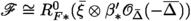
When h is the identity Thaddeus first shows that . But this follows because the higher direct images of under the map $\pi :\widetilde{M_{i}}\mapsto M_{i}$ vanish so the Leray spectral sequence implies and then since the projection formula implies . Similarly . Then, we can write for any $h\in G$

and

and one can work on $\widetilde{M_{i}}$.

Recall that $q_{i}=n-(i-1)m$. Next, one considers two cases.

1) When $q_{i}\le 0$, by definition of $B_{i,m,n}$ (see equation (4.8)), one has $N_{i}(h)=0$.

If $q_{i}= 0$ then we are done because on $\widetilde{M_{i}}$ by (5.6). So we assume now that $q_{i}< 0$.

Since $E_{i}$ is a G-invariant divisor on $\widetilde{M_{i}}$, the exact sequence induced by the embedding $E_{i}\hookrightarrow \widetilde{M_{i}}$

(5.7)

is a G-equivariant exact sequence of linearized sheaves so for each j we have an equivariant exact sequence

(5.8)

Thaddeus identify with the sheaf(or rather its pushforward to $\widetilde{M_{i}}$) $L_{i}^{m}(-q_{i}-j,-j)$. The last corresponds to a the tensor product $F_{1}\otimes F_{2}$ of sheaves on $E_{i}$ where $F_{1}$ is the pull-back of the sheaf $L_{i}^{m}$ ( defined in (4.3)) under the projection (here $\pi$ is $\pi _{1}\circ {\textsf{p}}_{1}= \pi _{2}\circ {\textsf{p}}_{2}$ in the diagram (5.3)) and (see equation (5.4)).

The exact sequence (5.8) induces a G-equivariant long exact sequence of cohomology groups from which we can write ( using the above identification):

(5.9)

Summing (5.9) over j, with $0<j\le -q_{i}$, and using (5.6) one arrives to

(5.10)

When h is the identity Thaddeus proves the vanishing of the right-hand side by showing that all the cohomology groups

$$\begin{aligned} H^{s}(E_{i},L_{i}^{m}(-q_{i}-j,-j)) \end{aligned}$$

vanish (all the direct images of $L_{i}^{m}(-q_{i}-j,-j)$ under the projection ${\textsf{p}}_{1}:E_{i}\rightarrow \mathbb {P}W_{i}^{-}$ vanish because

and for all t because $0<j<d+g-1-2i=\text{ rank } (W_{i}^{+})$ implies that a fibre ). Therefore the right-hand side of (5.10) vanish for any $h\in G$.

2) Now, we assume $q_{i}>0.$ Summing (5.9) over j, with $-q_{i}< j\le 0$, and using (5.6) one obtains

(5.11)

Now, the only non-zero direct image of ${L_{i}^{m}(-q_{i}+j,+j)}$ under the projection is the (i-1)-th (see (5.12) below):

given $D\in S^{i}X$ a fibre of $\pi$ is of the form ${E_{i}}_{D}=\mathbb {P}^{i-1}\times \mathbb {P}^{d+g-2-2i}$,

since $-q_{i}+j<0$ one has for $s\not =i-1$ and

since $j\ge 0$, for $s\not =0$.

So is the only non-zero Künneth component of .

To compute a direct image ${R^{i-1}_{\pi *}}_{}F$, one uses the fact that the Leray Spectral sequence $E_{2}^{t,s}={R^{t}_{\pi _{1}*}}_{}{R^{s}_{{\textsf{p}}_{1}*}}_{}F\Rightarrow$ ${R^{t+s}_{\pi *}}_{}F$. It will be enough to work with $F=$ because . We shall see that the only non-zero term of the Leray spectral sequence is $E_{2}^{i-1,0}$.

Notice that for all sheaves , the base change morphisms induced by the diagram (5.3) are isomorphisms, that is,

and for all $t\ge 0$.

Now, by the projection formula one has

(by the base change isomorphism) $=$

.

Since $j\ge 0$, for $s>0$ one has and for $s=0$ $S^{j}(W_{i}^{+})^{\vee }.$

Since $-q_{i}+j<0$ we have that unless $t= \text{ rank }(W_{i}^{-})-1 = i-1$ in which case

.

It follows that

$$\begin{aligned} {R^{i-1}_{\pi *}(L_{i}^{m}(-q_{i}+j,+j))=L_{i}^{m}\otimes \wedge ^{i}W_{i}^{-}\otimes S^{q_{i}-j-i}(W_{i}^{-})\otimes S^{j}(W_{i}^{+})^{\vee }}. \nonumber \\ \end{aligned}$$

(5.12)

By the Leray spectral sequence(the usual one) one has

$$\begin{aligned} {H^{s}(E_{i},L_{i}^{m}(-q_{i}+j,+j))=H^{s-(i-1)}(S^{i}X,R^{i-1}_{\pi *}(L_{i}^{m}(-q_{i}+j,+j)))}\nonumber \\ \end{aligned}$$

(5.13)

and the rest is a rather straightforward verification. One can write

$$\begin{aligned} \begin{aligned}&{L(h,E_{i},L_{i}^{m}(-q_{i}+j,+j))}\\&\quad = \sum _{s}{(-1)^{s}trace\left( h_{\mid }H^{s-(i-1)}(S^{i}X,R^{i-1}_{\pi *}(L_{i}^{m}(-q_{i}+j,+j)))\right) }\\&\quad =(-1)^{i-1}{L\left( h,S^{i}X,R^{i-1}_{\pi *}(L_{i}^{m}(-q_{i}+j,+j))\right) }.\\ \end{aligned} \end{aligned}$$

(5.14)

Multiplying (5.11) by $-1$ and using (5.14) we have

from (5.12) this is

$$\begin{aligned} =(-1)^{i}\sum _{j=0}^{q_{i}-1}{L\left( h,S^{i}X,L_{i}^{m}\otimes \wedge ^{i}W_{i}^{-}\otimes S^{q_{i}-j-i}(W_{i}^{-})\otimes S^{j}(W_{i}^{+})^{\vee }\right) }\\ \end{aligned}$$

and if $j>q_{i}-i$ then $S^{q_{i}-j-i}(W_{i}^{-})=0$ so in the last equation the sum becomes a sum that runs only from $j=0$ to $j=q_{i}-i$, that is

$$\begin{aligned}= & {} (-1)^{i}\sum _{j=0}^{q_{i}-i}{L\left( h,S^{i}X,L_{i}^{m}\otimes \wedge ^{i}W_{i}^{-}\otimes S^{q_{i}-j-i}(W_{i}^{-})\otimes S^{j}(W_{i}^{+})^{\vee }\right) }{}\\= & {} {(-1)^{i}L}\left( {{ h,S^{i}X,L_{i}^{m}\otimes \wedge ^{i}W_{i}^{-}\otimes }\left\{ \bigoplus _{j=0}^{q_{i}-i} { S^{q_{i}-j-i}(W_{i}^{-})\otimes S^{j}(W_{i}^{+})^{\vee }}\right\} }\right) \\{} & {} (\text{ using } \bigoplus _{j=0}^{q_{i}-i} {{ S^{q_{i}-j-i}(W_{i}^{-})\otimes S^{j}(W_{i}^{+})^{\vee }}}=S^{q_{i}-i}\left\{ {{ W_{i}^{-}\oplus (W_{i}^{+})^{\vee }}}\right\} )\\= & {} {(-1)^{i}L}\left( {{ h,S^{i}X,L_{i}^{m}\otimes \wedge ^{i}W_{i}^{-}\otimes S^{q_{i}-i}}\left\{ { W_{i}^{-}\oplus (W_{i}^{+})^{\vee }}\right\} }\right) \\= & {} {(-1)^{i}L}\left( {{ h,S^{i}X,L_{i}^{m}\otimes \wedge ^{i}W_{i}^{-}\otimes S^{q_{i}-i} U_{i}}}\right) \\= & {} {(-1)^{i}L}\left( {{ h,S^{i}X,B_{i,m,n}}}\right) \\= & {} {(-1)^{i}N_{i}(h)}. \end{aligned}$$

$\square$

Lemma 5.4

For $i>b$, $N_{i}(h)=0$.

Proof

This is the same proof of (6.8) in [32] since one shows that $i>b$ implies $q_{i}-i<0$ so $B_{i,m,n}=0$. $\square$

Finally, from Lemmas 5.1–5.4, one has

Therefore $Trace( h_{\mid _{ V_{m,n}}} )=\sum _{i=0}^{w}(-1)^{i}N_{i}(h)$.

6 The Chern classes

Let h be an automorphism of the curve X and assume that h has order $p\not = 1$. We shall explain below that the k-dimensional components of fixed points of h in the symmetric product $S^{i}X$ are parametrized by certain kind of h-invariant divisors so we represent such a component by $Z_{D}$, where D is the corresponding invariant divisor. Let $\iota _{D}$ denote the inclusion $Z_{D}\subset S^{i}X$. Consider the decompositions into eigenbundles

$$\begin{aligned} \iota _{D}^{*}W^{-}_{i}=\bigoplus _{j=1}^{p} \iota _{D}^{*}W^{-}_{i}(\nu ^{j}) \end{aligned}$$

(6.1)

and

$$\begin{aligned} \iota _{D}^{*}W^{+}_{i}=\bigoplus _{j=1}^{p} \iota _{D}^{*}W^{+}_{i}(\nu ^{j}). \end{aligned}$$

(6.2)

For the proof of Theorem 8.1 in Sect. 8, we need to know the Chern classes of all these eigenbundles and before we compute them we recall from [23] Section 3, that a k-dimensional component of fixed points of h in $S^{i}X$ is isomorphic to the symmetric product $S^{k}Y$, here Y is the quotient curve $X/\langle h\rangle$. These components are parametrized by a set of certain kind of h-invariant divisors $A_{k}$ of degree $d_{k}=i-pk$, hence the notation $Z_{D}$. More precisely, define $A_{k}$ as the set of divisors $D\in {(S^{d_{k}}X)}^{h}$ satisfying the following property: if $x\in X$ is a point in the support of D then $D-\sum _{j=0}^{p-1}h^{j}x$ is not an effective divisor nor the zero divisor. For each $D\in A_{k}$ there is an embedding

(6.3)

where $\iota$ sends $P\in S^kY$ to the divisor $f^*P\in S^{pk}X$ ( $f:X\rightarrow Y=X/\langle h\rangle$ is the quotient map) and sends $P\in S^{pk}X$ to $P+D\in S^{pk+d_{k}}X$.

Then, the Chern classes of our eigenbundles can be expressed in terms of the cohomology classes $\theta ,x$ and $\sigma _{i}\in H^2(S^kY,{\mathbb {Z}})$ (see [22] for details on cohomology of symmetric products), where x represents the class of a divisor $q+ S^{k-1}Y\subset S^kY$ in $H^2(S^kY,{\mathbb {Z}})$ and $\theta$ represents the class of the pull back of the theta divisor class $\Theta \in H^2(J_{Y},{\mathbb {Z}})$ of the Jacobian $J_{Y}$ of the curve Y under the Abel Jacobi map. We recall some relations of these cohomology classes:

$$\begin{aligned} \theta =\sum _{i=1}^{g_{Y}}\sigma _{i}, \,\,\sigma _{i}\sigma _{j}= \sigma _{j}\sigma _{i}, \text{ and } \sigma _{i}^{2}=0. \end{aligned}$$

(6.4)

If $0\le a\le g_{Y}$ and $0\le d$, then

$$\begin{aligned} \sigma _{i_{1}}\sigma _{i_{2}}\dots \sigma _{i_{a}}x^{d}= & {} x^{a+d} , \text{ for } \text{ distinct } i_{1}, i_{2},\dots ,i_{a}\text{. } \text{ Also } \end{aligned}$$

(6.5)

$$\begin{aligned} \theta ^{a}x^{d}= & {} a!\left( {\begin{array}{c}g_{Y}\\ a\end{array}}\right) x^{a+d} \text{ and } \end{aligned}$$

(6.6)

$$\begin{aligned} e^{z\theta }= & {} \prod _{i=1}^{g_{Y}}(1+z\sigma _{i}). \end{aligned}$$

(6.7)

The Todd class $Td(Z_{D})$ of a k-dimensional component is given by

$$\begin{aligned} Td(Z_{D})=Td(S^{k}Y)=\left( \frac{x}{1-e^{-x}}\right) ^{k-g_{Y}+1}exp\left( \frac{\theta }{e^{x}-1}-\frac{\theta }{x}\right) , \end{aligned}$$

(6.8)

see for instance (7.3) in [32], there $\sigma =\theta$ and $\eta =x$.

Let $D\in A_{k}$. We will consider as well the following decomposition into eigenbundles on Y

$$\begin{aligned} f_{*}(\xi ^{s}(-nD))=\bigoplus ^{p-1}_{j=0}\lambda _{s,j,n}, \end{aligned}$$

(6.9)

here $\lambda _{s,j,n}:=f_{*}(\xi ^{s}(-nD))(\nu ^{j})$. We have the following

Theorem 6.1

Let $Z_{D}$ be a k-dimensional component of fixed points of h in $S^{i}X$. Let $m_{j,1},m_{j,2},$ $m'_{j,n}$ denote the degrees of the bundles $\lambda _{1,j,1}$,$\lambda _{1,j,2}$ and $\lambda _{-1,j,n}$,respectively, in formula (6.9). Let $g_{Y}$ be the genus of the quotient curve Y. Then,

• (a) For the eigenbundles in (6.2), their corresponding Chern characters and classes are given by:

  $$\begin{aligned} ch(\iota _{D}^{*}W^{+}_{i}(\nu ^{j}))=-e^{2x}(1+m'_{j,-2}-(-2k+g_{Y}+4\theta )) \end{aligned}$$

  (6.10)

  and

  $$\begin{aligned} c(\iota _{D}^{*}W^{+}_{i}(\nu ^{j}))=\frac{e^{\frac{4\theta }{1+2x}}}{(1+2x)^{(1+m'_{j,-2}+2k-g_{Y})}}. \end{aligned}$$

  (6.11)

• (b) For the eigenbundles in equation (6.1) we have:

  $$\begin{aligned} ch(\iota _{D}^{*}W^{-}_{i}(\nu ^{j}))= & {} e^{-x}(1+m_{j,1}-(k+g_{Y}+\theta ))\nonumber \\{} & {} -e^{-2x}(1+m_{j,2}-(2k+g_{Y}+4\theta )) \end{aligned}$$

  (6.12)

  and

  $$\begin{aligned} c(\iota _{D}^{*}W^{-}_{i}(\nu ^{j}))=\frac{(1-x)^{1+m_{j,1}-k-g_{Y}}}{(1-2x)^{1+m_{j,2}-2k-g_{Y}}} e^{-\frac{\theta }{1-x}+\frac{4\theta }{1-2x}}. \end{aligned}$$

  (6.13)

In the diagrams (6.14), (6.16)and (6.18) below we introduce notation for some morphisms that appear in the proof of Theorem 6.1 and of Lemma 6.1. In the diagram (6.14) $\rho _{S^{k}Y}$ and $\pi _{S^i X}$ are the natural projections, $\iota _{D}$ is the embedding (6.3) corresponding to the component $Z_{D}$, $j'$ stands for the embedding of the universal divisor $\Delta _{i}$ of $S^{i}X$,

and $\beta '$ is the corresponding embedding into $X\times S^{k}Y$.

According to (6.3), we have

(6.15)

and the diagram (6.14) can be subdivided as in (6.16) below

We will also consider the universal divisor $\Delta _{pk}$ of $S^{pk}X$ and the projections

• $\pi _{X}:X\times S^{i}X\rightarrow X$,

• ${\textsf{p}}_{X}:X\times S^{pk}X\rightarrow X$ and

• ${\rho _{X}}:X\times S^{k}Y\rightarrow X$.

The diagram (6.18) involves the projection $\rho _{S^{k} Y}$ which is decomposed as ${\pi }_{S^{k}Y}\circ F$, where $F=f\times Id_{S^{k} Y}$ and ${\pi _{S^{k} Y}}$ is the projection $Y\times S^{k}Y\mapsto S^{k}Y$. We will often use the line bundle

${{\bar{\xi }}}=\rho _{X}^{*}\xi$ on $X\times S^{k}Y$.

For example, we have

$$\begin{aligned} ( Id_{X}\times \iota _{D})^{*}(\xi ^{-1}(2\Delta _{i}))\cong {\bar{\xi }} ^{-1}(2{\overline{{\Delta } }}). \end{aligned}$$

(6.17)

Lemma 6.1

Let $\Delta _{Y}$ be the universal divisor of $S^{k}Y$.Consider the line bundles ${\bar{\xi }}={\rho _{X}}^{*}\xi$ on $X\times S^{k}Y$ and on $Y\times S^{k}Y$ . Then we have for

(6.19)

In particular, the $\nu ^{j}$-eigenbundles of and are given by

(6.20)

(6.21)

Proof

Since $\rho _{S^{k} Y}={\pi }_{S^{k}Y}\circ F$, ( $F=f\times Id_{S^{k} Y}$) and F has finite fibres one can write

(6.22)

Next, we shall write in terms of the universal divisor $\Delta _{pk}$ of $S^{pk}X$ and of the divisor D (see formula (6.24) below). We have (by definition of and equation (6.15))

(6.23)

and by the universal property of $\Delta _{i}$ applied to the right-hand side square of the diagram (6.16) one has that is the relative divisor of degree i inducing . So we have

and using this in (6.23), we get

(6.24)

Now, using (6.24) in (6.22) and the fact that

$$\begin{aligned} (Id_{X}\times \iota )^{*}\Delta _{pk}=F^{*}\Delta _{Y} \end{aligned}$$

we have

Applying the projection formula to the direct image $R^{0}_{F*}$ one gets

Now we use the following base change isomorphism induced from the left-hand side square of (6.18)

$$\begin{aligned} R^{0}_{F*}\{ \rho _{X}^{*}(\xi ^{s}(-nD))\} \cong \pi _{Y}^{*} f_{*}(\xi ^{s}(-nD)) \end{aligned}$$

(6.25)

to get

and using the decomposition into eigenbundles (6.9) we get

Notice that given $f:X\rightarrow Y$ with X Noetherian, the higher direct images commute with direct sums namely $R^{j}f_{*}(\bigoplus _{i} {\mathscr {F}}_{i})=\bigoplus _{i}R^{j}f_{*}({\mathscr {F}}_{i})$. So we have

(6.26)

from which the Lemma follows. $\square$

Lemma 6.2

Let Y be an irreducible non singular projective curve of genus $g_{Y}$. Consider the projection $\pi _{S^{k}Y}:Y\times S^{k}Y\rightarrow S^{k}Y$ in (6.18) and the universal divisor $\Delta _{Y}\subset Y\times S^{k}Y$. For any line bundle M on Y and any $m\in \mathbb {Z}$ we have the following Chern character

$$\begin{aligned} ch \ \big ((\pi _{S^{k}Y})_{!}\pi _{Y}^{*}M(m\Delta _{Y})\big )=((deg \ M+mk+1-g_{Y})-m^{2}\theta )e^{m x}, \end{aligned}$$

(6.27)

where .

Proof

This is (7.4) in [32] setting $X=Y$, $g=g_{Y}$, $i=k$, $\pi =\pi _{S^{k}Y}$ (for Thaddeus $\pi :X\times S^{i}X\rightarrow S^{i}X$), $k=m\in \mathbb {Z}$ and also recall that for Thaddeus $\sigma =\theta$ and $\eta =x$. $\square$

Proof of Theorem 6.1

(a) We first notice that

$$\begin{aligned} \iota _{D}^{*}W^{+}_{i}\cong & {} R^{1}_{\rho _{S^{k} Y}*}( Id_{X}\times \iota _{D})^{*}(\xi ^{-1}(2\Delta _{i})). \end{aligned}$$

(6.28)

By definition (equation (4.2)) we have $\iota _{D}^{*}W^{+}_{i}=\iota _{D}^{*}(R^1_{\pi _{S^{i}X}})_{*}\xi ^{-1}(2\Delta _{i})$ then (6.28) follows because under our conditions the natural base change morphism

$$\begin{aligned} \iota _{D}^{*}(R^j_{\pi _{S^{i}X}})_{*}\xi ^{-1}(2\Delta _{i}) \mapsto R^{j}_{\rho _{S^{k} Y}*}( Id_{X}\times \iota _{D})^{*}(\xi ^{-1}(2\Delta _{i})), \end{aligned}$$

(6.29)

induced from diagram (6.14), is an isomorphism $\forall \ j\ge 0$. That is, from Corollary 2 pg. 50 in [26] we see that the higher direct images $(\!R^j_{\pi _{S^{i}X}}\!)_{*}\xi ^{-1}(\!2\Delta _{i}\!)$, $j\ge 0$, are locally free sheaves and that for any $y\in S^{i}X$ the natural maps

$$\begin{aligned} \phi ^{j}_{y}:(R^j_{\pi _{S^{i}X}})_{*}\xi ^{-1}(2\Delta _{i})\otimes k(y)\mapsto H^{j}((X\times S^{i}X)_{y}, \xi ^{-1}(2\Delta _{i})_{y}) \end{aligned}$$

are isomorphisms (in fact, the only ones that are non-zero are $(\!R^1_{\pi _{S^{i}X}}\!)_{*}\xi ^{-1}(\!2\Delta _{i}\!)$ and $\phi ^{1}_{y}$). So the isomorphism in (6.29) follows as a particular case of Corollary 6.9.9.2 in [18] or from Theorem 2.1 in [11].

Since (by equation (6.17))

we have for the $\nu ^{j}$-eigenbundles

(6.30)

Now by equation (6.28) the left-hand side of (6.30) is $\iota ^{*}_{D}W_{i}^{+}(\nu ^{j})$ and the right-hand side is by Lemma 6.1 (equation (6.20) taking n=-2, s=-1) . That is

(6.31)

so that using the Grothendieck-Riemann-Roch Theorem one can compute the Chern characters $ch(\iota _{D}^{*}W^{+}(\nu ^{j}))$. In fact, $ch(\iota _{D}^{*}W^{+}(\nu ^{j}))$ can be derived from Lemma 6.2, that is, consider so taking $M=\lambda _{s,j,n}$ we have $deg \ M=deg \ \lambda _{s,j,n}$ and in our case $s=-1$ and $n=-2$ so $deg \ M=m'_{j,-2}$ ($m'_{j,n}$ as defined in the statement of Theorem 6.1) and so taking $m=2$ Lemma 6.2 tell us that

we will see below that so we have that

that is

$$\begin{aligned} ch(\iota _{D}^{*}W^{+}_{i}(\nu ^{j}))=-e^{2x}(1+m'_{j,-2}-(-2k+g_{Y}+4\theta )). \end{aligned}$$

(6.32)

Now because if

then because by Lemma 6.1 we know that

Now we have (again by equation (6.17)) that

and as we mention in the proof of (6.29)

$$\begin{aligned} R^{0}_{\rho _{S^{k} Y}*}( Id_{X}\times \iota _{D})^{*}(\xi ^{-1}(2\Delta _{i}))=0. \end{aligned}$$

On the other hand, using (6.7) one has the factorization

$$\begin{aligned} \frac{e^{\frac{4\theta }{1+2x}}}{(1+2x)^{(1+m'_{j,-2}+2k-g_{Y})}}= (1+2x)^{(r''-g_{Y})}\cdot \prod _{i=1}^{g_{Y}}(1+4\sigma _{i}+2x), \end{aligned}$$

(6.33)

where $r''=-1-m_{j,-2}-2k+g_{Y}$. So (6.33) can be seen as the Chern class $c(L^{\oplus (r''-g_{Y})}\oplus ( L\otimes E))$, where L is a line bundle with Chern class $1+2x$ and E is a rank $g_{Y}$ vector bundle with $c(E)=e^{4\theta }$. Now we see, by properties of the Chern character and (6.32), that

$$\begin{aligned} ch(L^{\oplus (r''-g_{Y})}\oplus ( L\otimes E))= & {} ch(L^{\oplus (r''-g_{Y})})+ ch( L)ch( E)\\= & {} e^{2x}(r''-g_{Y})+e^{2x}(g_{Y}+4\theta )\\= & {} ch(\iota _{D}^{*}W^{+}_{i}(\nu ^{j})). \end{aligned}$$

So we have $c(L^{\oplus (r''-g_{Y})}\oplus ( L\otimes E))= c(\iota _{D}^{*}W^{+}_{i}(\nu ^{j}))$.

proof of b):

Using the definition of $W_{i}^{-}$ (equation (4.1)), we have

$$\begin{aligned} \iota ^{*}_{D}W_{i}^{-}= \iota ^{*}_{D}(R^0_{\pi _{S^{i}X}})_{*}{\mathscr {E}} \end{aligned}$$

where

is a flat sheaf on $X\times S^{i}X$ because $(R^0_{\pi _{S^{i}X}})_{*}{\mathscr {E}}=W^{-}_{i}$ is a locally free sheaf on $S^{i}X$. One can argue similarly as in the proof of a) to get the following base change isomorphism induced by the diagram (6.14)

$$\begin{aligned} \iota ^{*}_{D}(R^0_{\pi _{S^{i}X}})_{*}{\mathscr {E}}\cong (R^{0}_{\rho _{S^{k}Y}})_{*}(Id_{X}\times \iota _{D})^{*}{\mathscr {E}} \end{aligned}$$

that is

$$\begin{aligned} \iota _{D}^{*}W^{-}_{i} \cong (R^{0}_{\rho _{S^{k}Y}})_{*}(Id_{X}\times \iota _{D})^{*}{\mathscr {E}}. \end{aligned}$$

One can see that

(6.34)

(by using the base change isomorphism induced by the square diagram obtained on the top of the diagram (6.14) by adding the natural projection ). Then

(6.35)

Consider the exact sequence of sheaves on $X\times S^{k}Y$

(6.36)

Since F has finite fibres we get an exact sequence of sheaves on $Y\times S^{k}Y$

(6.37)

which induces, for each $j=0,1\cdots p-1$, an exact sequence of $\nu ^{j}$-eigen sheaves

(6.38)

We continue by making the following observations.

• (1) Let

  

  Notice that (by the projection formula) is the non-zero term on the right-hand side of the exact sequence of (6.37).

• (2) We have ${\mathscr {F}}=\bigoplus _{j} {\mathscr {F}}(\nu ^{j})$ and then $R^{0}_{\pi _{S^{k}Y}*}{\mathscr {F}}=\bigoplus _{j}R^{0}_{\pi _{S^{k}Y}*}\{{\mathscr {F}}(\nu ^{j})\}$. Since $R^{0}_{\pi _{S^{k}Y}*}\{{\mathscr {F}}(\nu ^{j})\}$ inherits the action of h from ${\mathscr {F}}(\nu ^{j})$ we see that

  $$\begin{aligned} \{R^{0}_{\pi _{S^{k}Y}*}{\mathscr {F}}\}(\nu ^{j})=R^{0}_{\pi _{S^{k}Y}*}\{{\mathscr {F}}(\nu ^{j})\}. \end{aligned}$$

• (3) From (6.35) $R^{0}_{\pi _{S^{k}Y}*}\{{\mathscr {F}}\}\cong \iota _{D}^{*}W^{-}_{i}$ so we get that

  $$\begin{aligned} \iota _{D}^{*}W^{-}_{i}(\nu ^{j})\cong R^{0}_{\pi _{S^{k}Y}*}\{{\mathscr {F}}(\nu ^{j})\} \end{aligned}$$

  for $j=0,\cdots , p-1$.

• (4) Also notice that is the non-zero term on the right-hand side of the exact sequence of (6.38).

• (5) From (6.38) we have the following identity in the Grothendieck ring $K(Y\times S^kY)$

  

  So applying $\pi _{S^{k}Y!}:K(Y\times S^kY)\rightarrow K(S^kY)$ followed by the Chern character ch one has that

  

  (6.39)

• (6) For $s\ge 1$ we have

  

  and consequently $R^{s}_{\pi _{S^{k}Y}*}\{{\mathscr {F}}(\nu ^j)\}=0$.

With (3) and (6) in (6.39) above we see that

(6.40)

Applying Lemma 6.2 to each character in (6.40) with $M = \lambda _{1,j,1}$ for the first one and $M=\lambda _{1,j,2}$ for the second one we have

$$\begin{aligned} \begin{aligned} ch(i^{*}_{D}W^{-}_{i}(\nu ^{j}))&= e^{-x}(1+m_{j,1}-(k+g_{Y}+\theta ))\\&\quad -e^{-2x}(1+m_{j,2}-(2k+g_{Y}+4\theta )). \end{aligned} \end{aligned}$$

(6.41)

(7) For the calculation of the Chern class we write

$$\begin{aligned} ch(i^{*}_{D}W^{-}_{i}(\nu ^{j}))= e^{-x}(r-\theta ))+e^{-2x}(r'+4\theta ), \end{aligned}$$

(6.42)

where $r=1+m_{j,1}-k-g_{Y}$ and $r'=-1-m_{j,2}+2k+g_{Y}$. Assume $r,r'\ge g_{Y}$. Then

$$\begin{aligned} ch(i^{*}_{D}W^{-}_{i}(\nu ^{j}))= ch((L_{1}\otimes E_{1}) \oplus (L_{2}\otimes E_{2} )),\end{aligned}$$

where $L_{1}$ and $L_{2}$ are line bundles with Chern classes $1-x$ and $1-2x$ respectively and $E_{1}$ and $E_{2}$ are vector bundles with Chern characters $r-\theta$ and $r'+4\theta$ respectively. So,

$$\begin{aligned} c(i^{*}_{D}W^{-}_{i}(\nu ^{j}))= c(L_{1}\otimes E_{1}) \cdot c(L_{2}\otimes E_{2} ). \end{aligned}$$

From (6.4), one can assume that the non-zero Chern roots of $E_{1}$ and $E_{2}$ are $-\sigma _1,\dots , -\sigma _{g_{Y}}$ and $4\sigma _1,\dots , 4\sigma _{g_{Y}}$ respectively, so that

$$\begin{aligned} c(i^{*}_{D}W^{-}_{i}(\nu ^{j}))= & {} ((1-x)^{r-g_{Y}}\prod _{i=1}^{g_{Y}}(1-x-\sigma _{i}))\nonumber \\{} & {} \cdot ( (1-2x)^{r'-g_{Y}}\prod _{i=1}^{g_{Y}}(1-2x+4\sigma _{i}) ) \end{aligned}$$

(6.43)

and using (6.7) the last is

$$\begin{aligned} =(1-x)^{r}e^{\frac{-\theta }{1-x}}(1-2x)^{r'}e^{\frac{4\theta }{1-2x}}. \end{aligned}$$

(6.44)

In case $r,r'\not \ge g_{Y}$ one argues similarly by choosing integers $s,s'$ so that $r+s,r'+s'\ge g_{Y}$, then adding $e^{-x}s+e^{2x}s'$ to both sides of (6.42) one has

$$\begin{aligned} ch(i^{*}_{D}W^{-}_{i}(\nu ^{j}))+e^{-x}(s)+e^{2x}(s')= e^{-x}(r+s-\theta ))+e^{-2x}(r'+s'+4\theta ), \end{aligned}$$

which can be seen as

$$\begin{aligned} ch(i^{*}_{D}W^{-}_{i}(\nu ^{j})\oplus L_{1}^{\oplus s} \oplus L_{2}^{\oplus s'} )=ch((L_{1}\otimes F_{1})\oplus (L_{2}\otimes F_{2})), \end{aligned}$$

where $F_{1}, F_{2}$ have ranks $r+s$ and $r+s'$ respectively. So

$$\begin{aligned} c(i^{*}_{D}W^{-}_{i}(\nu ^{j})\oplus L_{1}^{\oplus s} \oplus L_{2}^{\oplus s'} )=c((L_{1}\otimes F_{1})\oplus (L_{2}\otimes F_{2})), \end{aligned}$$

and by (6.44) we can compute the right-hand side, namely

$$\begin{aligned} c(i^{*}_{D}W^{-}_{i}(\nu ^{j})\oplus L_{1}^{\oplus s} \oplus L_{2}^{\oplus s'} )=(1-x)^{r+s}e^{\frac{-\theta }{1-x}}(1-2x)^{r'+s'}e^{\frac{4\theta }{1-2x}}, \end{aligned}$$

and we also get

$$\begin{aligned} \begin{aligned} c(i^{*}_{D}W^{-}_{i}(\nu ^{j}))&=(1-x)^{r+s}e^{\frac{-\theta }{1-x}}(1-2x)^{r'+s'}e^{\frac{4\theta }{1-2x}}(c(L_{1}^{\oplus s}))^{-1}(c((L_{2}^{\oplus s'}))^{-1} \\&=(1-x)^{r+s}e^{\frac{-\theta }{1-x}}(1-2x)^{r'+s'}e^{\frac{4\theta }{1-2x}}(1-x)^{-s}(1-2x)^{-s'} \\&=(1-x)^{r}e^{\frac{-\theta }{1-x}} (1-2x)^{r'}e^{\frac{4\theta }{1-2x}}. \end{aligned} \end{aligned}$$

(6.45)

$\square$

7 Stable characteristic classes

Theorem 7.1 below is a generalization of Theorem 2.3 in [24] where the case $D=0$ is considered. The proof, which we have omitted here, can be done using similar arguments to those in the proof of Theorem 6.1 above.

Theorem 7.1

Let $Z_{D}$ be a k-dimensional component of fixed points of h in $S^{i}X$. Let $n_{j}$ and $n_{j}'$ be the degrees of the line bundles $\lambda _{0,j,-1}$ and $\lambda _{0,j,0}$ in formula (6.9) respectively. Then

$$\begin{aligned}{} & {} \mathrm{(a)} \, ch(N_{Z_{D}/S^{i}X}(\nu ^{j}))=-(1+n'_{j}-g_{Y})+e^{x}(1+n_{j}+k-g_{Y}-\theta ), \end{aligned}$$

(7.1)

$$\begin{aligned}{} & {} \mathrm{(b)} \, c(N_{Z_{D}/S^{i}X}(\nu ^{j}))=(1+x)^{1+n_{j}+k-g_{Y}}e^{-\frac{\theta }{1+x}}, \end{aligned}$$

(7.2)

$$\begin{aligned}{} & {} \mathrm{(c)} \, U_{j}(N_{Z_{D}/S^{i}X}(\nu ^{j}))=\left( 1-\frac{1}{\nu ^{j}}\right) ^{A}\left( 1-\frac{e^{-x}}{\nu ^{j}}\right) ^{-A} exp\left( \frac{\theta e^{-x}}{\nu ^{j}-e^{-x}}\right) \nonumber \\{} & {} \quad \cdot \left( \frac{1-e^{-x}/\nu ^{j}}{1-\nu ^{-j}}\right) ^{-n_{j}}, \end{aligned}$$

(7.3)

$$\begin{aligned}{} & {} \mathrm{(d)} \, \prod ^{p-1}_{j=1}U_{j}(N_{Z_{D}/S^{i}X}(\nu ^{j}))=p^{A}m(e^{-x})^{-A} e^{\theta q(e^{-x})}\prod ^{p-1}_{j=1}\left( \frac{1-e^{-x}/\nu ^{j}}{1-\nu ^{-j}}\right) ^{-n_{j}},\nonumber \\ \end{aligned}$$

(7.4)

where $A=k+1-g_{Y}$, $m(z)=\sum ^{p-1}_{j=0}z^{i}$ and $\ q(z)=\frac{-zm'(z)}{m(z)}$.

In particular, we have

$$\begin{aligned} {\text {det}(Id-h_{\mid }{N^{\vee }_{Z_{D}/{S^{i}X}}})}={(1-\nu ^{p-1})^{a_{1}}\cdot \cdot \cdot (1-\nu )^{a_{p-1}}} \end{aligned}$$

(7.5)

where

$$\begin{aligned} a_{j}= \textrm{rank}(N_{Z_{D}/S^{i}X}(\nu ^{p-j}))=(n_{p-j}-n'_{p-j}+k) \text{ by } \text{ part } \text{ a). } \end{aligned}$$

8 The generalized Chern character for $B_{i,m,n}$

Let $Z_{D}$ be a component of fixed points of the automorphism h. Let E and F be $h-$linearized vector bundles on $Z_{D}$. The generalized Chern character of E is given by

$$\begin{aligned} ch_{h}(E)=\sum _{j=0}^{p-1}\nu ^{j}ch[E(\nu ^{j})], \end{aligned}$$

where $ch[E(\nu ^{j})]$ is the Chern character of the eigenbundle $E(\nu ^{j})$. As in the case of the usual Chern character one has that

$$\begin{aligned} ch_{h}(E\otimes F)=ch_{h}(E)ch_{h}(F). \end{aligned}$$

So, from equation (4.8) we have

$$\begin{aligned} ch_{h}(\iota ^{*}_{D}B_{i,m,n})=ch_{h}(\iota ^{*}_{D}L^{m}_{i})ch_{h}(\wedge ^{i}\iota ^{*}_{D}W^{-}_{i}) ch_{h}(\iota ^{*}_{D}S^{q_{i}-(i)}U_{i}). \end{aligned}$$

(8.1)

The factors on the right-hand side of (8.1) are given in the following result.

Theorem 8.1

Let $Z_{D}$ be a k-dimensional component of fixed points of h in $S^{i}X$. Let $g_{Y}$ be the genus of the quotient curve Y. Let $d_{k}=i-pk$ be the degree of D. Let $\nu ^{l}$ and $\nu ^{l'}$ be the eigenvalues corresponding to the action of h on the line-bundles $\iota ^{*}_{D}L_{i}$ and $\wedge ^{i}\iota ^{*}_{D}W^{-}_{i}$ respectively.

We have the following

$$\begin{aligned}{} & {} (a) \, ch_{h}(\iota ^{*}_{D}L^{m}_{i})=\nu ^{lm} \cdot e^{m(d-2i)x+2mp\theta }. \end{aligned}$$

(8.2)

$$\begin{aligned}{} & {} (b) \, ch_{h}(\wedge ^{i}\iota ^{*}_{D}W^{-}_{i}) =\nu ^{l'}\cdot e^{(d-3i+1-g_{X})x+3p\theta }. \end{aligned}$$

(8.3)

(c) Let $m_{j,n}$ and $m'_{j,n}$ denote respectively the degrees of the bundles $\lambda _{1,j,n}$ and $\lambda _{-1,j,n}$ in formula (6.9) .Then

$$\begin{aligned}{} & {} ch_{h}(\iota _{D}^{*}S^{q_{i}-i}U_{i})=\nonumber \\{} & {} \quad =\underset{t^{q_{i}-i}}{coef}\left[ exp\left( \frac{-pt^{p}\theta }{e^{px}-t^{p}} \right) \cdot \frac{(1-t^{p}e^{-px})^{k+g_{Y}-1}}{(1-t^{p}e^{-2px})^{2g_{Y}-2}}\right. \nonumber \\{} & {} \left. \cdot \prod _{j=0}^{p-1}\left\{ \frac{(1-\nu ^{j}te^{-2x})^{m_{j,2}+m'_{p-j,-2}}}{(1-\nu ^{j}te^{-x})^{m_{j,1}}} \right\} \right] . \end{aligned}$$

(8.4)

Proof

Parts a) and b) follow from (7.5) in [32] and the restriction rules $\iota ^{*}_{D}\theta =p\theta$ and $\iota ^{*}_{D}x=x$, where we are using the same notation for the cohomology classes of the symmetric products $S^{i}X$ and $S^{k}Y\cong Z_{D}$ as introduced in Sect. 6 above (recall that for Thaddeus $\sigma =\theta$ and $\eta =x$).

For (c), let E be a rank $r_E$ vector bundle on $Z_{D}$ and let

$$\begin{aligned} P(E,t):=\sum _{l=0}^{\infty }ch[S^{l}(E)]\cdot {t}^{l}. \end{aligned}$$

(8.5)

One has (see proof of (7.6) in [32])

$$\begin{aligned} P(E,t)=\prod _{\begin{array}{c} \text{ Chern } \text{ roots } \alpha \text { of }E,\\ \end{array}} \frac{1}{1-te^{\alpha }}. \end{aligned}$$

(8.6)

Let F be an h-linearized vector bundle on $Z_{D}$ and let

$$\begin{aligned} Q_{h}(F,t)=\sum _{l=0}^{\infty }ch_{h}(S^{l}F)\cdot t^{l}. \end{aligned}$$

(8.7)

Since $S^{l}F=\bigoplus _{j=0}^{p-1}(S^{l}F)(\nu ^{j})$, a Chern root $\gamma$ of $S^{l}F$ is a Chern root of $(S^{l}F)(\nu ^{j})$ for some j, say $\gamma =\sum _{i=1}^{s}\beta _{i}\alpha _{i}$ where $\beta _{i}\ge 0$, $\sum _{i=1}^{s}\beta _{i}=l$ and $\alpha _{i}$ is a Chern root of $F(\nu ^{j_{i}})$ for some integer $j_{i}$. Then $\nu ^{j}e^{\gamma }=m(\nu ^{j_{1}}e^{\alpha _{1}},\dots ,\nu ^{j_{s}}e^{\alpha _{s}})$ where m is the degree l monomial $m(x_{1},\dots ,x_{s})=\prod _{i=1}^{s}x_{i}^{\beta _{i}}$. So one has that

$$\begin{aligned} Q_{h}(F,t)=\prod _{\begin{array}{c} \text{ Chern } \text{ roots } \alpha \text{ of } F(\nu ^{j}),\\ j=0,\ldots ,p-1. \end{array}} \frac{1}{1-\nu ^{j}te^{\alpha }}, \end{aligned}$$

(8.8)

from which one sees that

$$\begin{aligned} Q_{h}(F,t)=\prod _{j=0}^{p-1}P(F(\nu ^{j}),\nu ^{j}t). \end{aligned}$$

(8.9)

Now we shall assume that $F=\iota _{D}^{*}U_{i}$ and compute $Q_{h}(F,t)$ using (8.9).

Using (4.6) and taking Chern class, we have that

$$\begin{aligned} c(F(\nu ^{j}))=c(\iota _{D}^{*}W^{-}_{i}(\nu ^{j}))\cdot c((\iota _{D}^{*}W^{+}_{i})^{\vee }(\nu ^{j})). \end{aligned}$$

(8.10)

From equations (6.43) and (6.33), one has the following factorizations

$$\begin{aligned} \begin{aligned}&c(\iota _{D}^{*}W^{-}_{i}(\nu ^{j}))=\\&\quad =(1-x)^{(r-g_{Y})}\cdot (1-2x)^{(r'-g_{Y})}\prod _{i=1}^{g_{Y}}(1-\sigma _{i}-x)\cdot \prod _{i=1}^{g_{Y}}(1+4\sigma _{i}-2x)\\&\quad =\prod _{\begin{array}{c} \text{ Chern } \text{ roots } \alpha \text{ of } \iota _{D}^{*}W^{-}_{i}(\nu ^{j})\\ \end{array}} (1+{\alpha }). \end{aligned}\nonumber \\ \end{aligned}$$

(8.11)

and

$$\begin{aligned} \begin{aligned} c((\iota _{D}^{*}W^{+}_{i})^{\vee }(\nu ^{j}))= (1-2x)^{(r''-g_{Y})}\cdot \prod _{i=1}^{g_{Y}}(1-4\sigma _{i}-2x),\\ =\prod _{\begin{array}{c} \text{ Chern } \text{ roots } \alpha \text{ of } (\iota _{D}^{*}W^{+}_{i})^{\vee }(\nu ^{j})\\ \end{array}} (1+{\alpha }).\\ \end{aligned}\nonumber \\ \end{aligned}$$

(8.12)

where

$$\begin{aligned} \begin{aligned} r&=1+m_{j,1}-k-g_{Y},\ \ \ \ \ \\ r'&=-1-m_{j,2}+2k+g_{Y} \ \ \ \text{ and } \\ r''&=-1-m'_{p-j,-2}-2k+g_{Y}. \end{aligned} \end{aligned}$$

(8.13)

So from (8.10), (8.11) and (8.12) we have the Chern roots of $F(\nu ^{j})$ and we use them in (8.6) to compute

$$\begin{aligned} P(F(\nu ^{j}),t)= & {} \left( \frac{1}{1-te^{-x}}\right) ^{r-g_{Y}}\cdot \prod _{i=1}^{g_{Y}}\left( \frac{1}{1-te^{-\sigma _{i}-x}}\right) \times \\{} & {} \times \left( \frac{1}{1-te^{-2x}}\right) ^{r'-g_{Y}}\cdot \prod _{i=1}^{g_{Y}}\left( \frac{1}{1-te^{4\sigma _{i}-2x}}\right) \cdot \left( \frac{1}{1-te^{-2x}}\right) ^{r''-g_{Y}}\\{} & {} \cdot \prod _{i=1}^{g_{Y}}\left( \frac{1}{1-te^{-4\sigma _{i}-2x}}\right) . \end{aligned}$$

Let $h(z):=\frac{1}{1-te^{-z}}$. Expanding the following around $\sigma _{i}=0$ and using $\sigma _{i}^{2}=0$ one has, as the reader may check, that

$$\begin{aligned} h(\sigma _{i}+x)= & {} \frac{1}{1-te^{-\sigma _{i}-x}}=h(x)\left( 1+\sigma _{i}\frac{h'(x)}{h(x)}\right) , \end{aligned}$$

(8.14)

$$\begin{aligned} h(-4\sigma _{i}+2x)= & {} \frac{1}{1-te^{4\sigma _{i}-2x}}=h(2x)\left( 1-4\sigma _{i}\frac{h'(2x)}{h(2x)}\right) \end{aligned}$$

(8.15)

and

$$\begin{aligned} h(4\sigma _{i}+2x)=\frac{1}{1-te^{-4\sigma _{i}-2x}}=h(2x)\left( 1+4\sigma _{i}\frac{h'(2x)}{h(2x)}\right) . \end{aligned}$$

(8.16)

Now we represent $P(F(\nu ^{j}),t)$ as the product $G_{1}G_{2}G_{3}$ of 3 factors defined below which we will modify using (8.14), (8.15) and (8.16):

$$\begin{aligned} G_{1}:= & {} \left( \frac{1}{1-te^{-x}}\right) ^{r-g_{Y }}\cdot \prod _{i=1}^{g_{Y}}\left( \frac{1}{1-te^{-\sigma _{i}-x}}\right) \\= & {} \left( \frac{1}{1-te^{-x}}\right) ^{r}\cdot \prod _{i=1}^{g_{Y}}\left( 1+\sigma _{i}\frac{h'(x)}{h(x)}\right) , \end{aligned}$$

using (6.7) one has that $\prod _{i=1}^{g_{Y}}\left( 1+\sigma _{i}\frac{h'(x)}{h(x)}\right) =e^{\left( \theta \frac{h'(x)}{h(x)}\right) }$. Also notice that $\frac{h'(x)}{h(x)}=-\frac{te^{-x}}{1-te^{-x}}=-\frac{t}{e^{x}-t}$ so

$$\begin{aligned} G_{1}=\left( \frac{1}{1-te^{-x}}\right) ^{r }\cdot e^{\left( \theta \frac{h'(x)}{h(x)}\right) } =(1-te^{-x})^{-r }\cdot exp\left( \frac{-t\theta }{e^{x}-t}\right) . \end{aligned}$$

(8.17)

In a similar way, we compute

$$\begin{aligned} G_{2}:= & {} \left( \frac{1}{1-te^{-2x}}\right) ^{r'-g_{Y}}\cdot \prod _{i=1}^{g_{Y}}\left( \frac{1}{1-te^{4\sigma _{i}-2x}}\right) \nonumber \\= & {} \left( \frac{1}{1-te^{-2x}}\right) ^{r'}\cdot \prod _{i=1}^{g_{Y}}\left( 1-4\sigma _{i}\frac{h'(2x)}{h(2x)}\right) \nonumber \\= & {} \left( \frac{1}{1-te^{-2x}}\right) ^{r'}\cdot e^{\left( -4\theta \frac{h'(2x)}{h(2x)}\right) } =(1-te^{-2x})^{-r'}\cdot exp\left( \frac{4t\theta }{e^{2x}-t}\right) \nonumber \\ \end{aligned}$$

(8.18)

and

$$\begin{aligned} G_{3}:= & {} \left( \frac{1}{1-te^{-2x}}\right) ^{r''-g_{Y}}\cdot \prod _{i=1}^{g_{Y}}\left( \frac{1}{1-te^{-4\sigma _{i}-2x}}\right) \nonumber \\= & {} \left( \frac{1}{1-te^{-2x}}\right) ^{r''}\cdot \prod _{i=1}^{g_{Y}}\left( 1+4\sigma _{i}\frac{h'(2x)}{h(2x)}\right) \nonumber \\= & {} \left( \frac{1}{1-te^{-2x}}\right) ^{r''}\cdot e^{\left( 4\theta \frac{h'(2x)}{h(2x)}\right) } =(1-te^{-2x})^{-r''}\cdot exp\left( \frac{-4t\theta }{e^{2x}-t}\right) .\nonumber \\ \end{aligned}$$

(8.19)

Multiplying (8.17), (8.18) and (8.19) we get, using the values for $r,r'$ and $r''$ given in (8.13), that

$$\begin{aligned} \begin{aligned} P(F(\nu ^{j}),t)&= (1-te^{-x})^{-1-m_{j,1}+k+g_{Y}}\\&\quad \cdot exp\left( \frac{-t\theta }{e^{x}-t}\right) (1-te^{-2x})^{2+m_{j,2}+m'_{p-j,-2}-2g_{Y}} \end{aligned} \end{aligned}$$

(8.20)

and replacing t by $\nu ^{j}t$

$$\begin{aligned} \begin{aligned} P(F(\nu ^{j}),\nu ^{j}t)&= (1-\nu ^{j}te^{-x})^{-1-m_{j,1}+k+g_{Y}}\\&\quad \cdot exp\left( \frac{-\nu ^{j}t\theta }{e^{x}-\nu ^{j}t}\right) (1-\nu ^{j}te^{-2x})^{2+m_{j,2}+m'_{p-j,-2}-2g_{Y}}. \end{aligned}\nonumber \\ \end{aligned}$$

(8.21)

Now we use (8.21) in (8.9) and recalling that $\nu =e^{2i\pi /p}$ one can verify that

$$\begin{aligned} Q_{h}( F,t)= & {} exp\left( \frac{-pt^{p}\theta }{e^{px}-t^{p}} \right) \cdot \frac{(1-t^{p}e^{-px})^{k+g_{Y}-1}}{(1-t^{p}e^{-2px})^{2g_{Y}-2}}\nonumber \\{} & {} \cdot \prod _{j=0}^{p-1}\left\{ \frac{(1-\nu ^{j}te^{-2x})^{m_{j,2}+m'_{p-j,-2}}}{(1-\nu ^{j}te^{-x})^{m_{j,1}}} \right\} . \end{aligned}$$

(8.22)

Therefore,

$$\begin{aligned} ch_{h}(\iota _{D}^{*}S^{l}U_{i})= & {} \underset{t^{l}}{coef}(Q_{h}(F,t)) \\= & {} \underset{t^{l}}{coef}\left[ \exp \left( \frac{-pt^{p}\theta }{e^{px}-t^{p}} \right) \cdot \frac{(1-t^{p}e^{-px})^{k+g_{Y}-1}}{(1-t^{p}e^{-2px})^{2g_{Y}-2}}\right. \\{} & {} \left. \cdot \prod _{j=0}^{p-1}\left\{ \frac{(1-\nu ^{j}te^{-2x})^{m_{j,2}+m'_{p-j,-2}}}{(1-\nu ^{j}te^{-x})^{m_{j,1}}} \right\} \right] . \end{aligned}$$

In particular, if $l=q_{i}-i$, ($q_i$ as in equation (4.8)), one has

$$\begin{aligned} ch_{h}(\iota _{D}^{*}S^{q_{i}-(i)}U_{i})=\underset{t^{q_{i}-(i)}}{coef}(Q_{h}(F,t)) \end{aligned}$$

(8.23)

$\square$

9 The involution of a hyperelliptic curve

Putting all data available to us so far in formula (1.2) the contribution of a component $Z_{D}$ of fixed points in $S^{i}X$ of an automorphism h of order p to the number $N_{i}(h)$ is given by the following (see details in Section  11):

$$\begin{aligned} C_{i,Z_{D}}(h)= & {} \frac{p^{A}\nu ^{l'+lm}}{(1-\nu ^{p-1})^{a_{1}}\cdot \cdot \cdot (1-\nu )^{a_{p-1}}} \underset{t^{q_{i}-(i)}}{Coef}\,\underset{x=0}{Res}\Bigg \{ [m(e^{-x})]^{-A}\prod _{j=1}^{p-1}\left( \frac{1-\frac{e^{-x}}{\nu ^{j}}}{1-\nu ^{-j}}\right) ^{-n_{j}} \nonumber \\{} & {} \times e^{[d(1+m)-i(3+2m)+1-g_{X}]x}\cdot \frac{(1-t^{p}e^{-px})^{k+g_{Y}-1}}{(1-t^{p}e^{-2px})^{2g_{Y}-2}}\nonumber \\{} & {} \cdot \prod _{j=0}^{p-1}\left\{ \frac{(1-\nu ^{j}te^{-2x})^{m_{j,2}+m'_{p-j,-2}}}{(1-\nu ^{j}te^{-x})^{m_{j,1}}} \right\} \nonumber \\{} & {} \quad \times \left( \frac{x}{1-e^{-x}} \right) ^{k-g_{Y}+1}\nonumber \\{} & {} \cdot \frac{\left( 1+x\left[ q(e^{-x})+p(3+2m)-\frac{pt^{p}}{e^{px}-t^{p}}+\left( \frac{1}{e^{x}-1}-\frac{1}{x} \right) \right] \right) ^{g_{Y}}}{x^{k+1}}dx\Bigg \}, \end{aligned}$$

(9.1)

where $A=k+1-g_{Y},$

$$\begin{aligned} a_{j}= rank(N_{Z_{D}/S^{i}X}(\nu ^{p-j}))=(n_{p-j}-n'_{p-j}+k). \end{aligned}$$

The constants $l,l',n_{j},n'_{j},m_{j,2},m_{j,1}, m'_{p-j,-2}$ (for their definitions see Theorem 8.1, Theorem 7.1 and Theorem 6.1) appearing in formula (9.1) depend on the particular situation (the curve X, the automorphism h, the line bundle $\xi$) and in this section, we will compute them for the case where X is a hyperelliptic curve of genus $g=g_{X}$, the automorphism h is the hyperelliptic involution and $\xi =K_{X}^{2}$ (see Lemmas 9.1, 9.2 and 9.3 below).

For the involution of a hyperelliptic curve, the contribution $C_{i,Z_{D}}(h)$ to the Lefschetz number $N_{i}(h)$ does not depend on D but only on the dimension of $Z_{D}$, the dimension of $S^{i}X$ and the genus $g_{X}$ of X. So we write

$$\begin{aligned} C_{i,k,g_{X}}(h)=C_{i,Z_{D}}(h) \end{aligned}$$

(9.2)

for $Z_{D}$ a $k-$dimensional component. There are $2g_{X}+2$ fixed points of h in the curve X and there are $\left( {\begin{array}{c}2g_{X}+2\\ i-2k\end{array}}\right)$ $k-$dimensional components $Z_{D}$ of fixed points of h in $S^{i}X$ each one corresponding to a divisor D of degree $i-2k$ supported on $i-2k$ distinct fixed points of h. Notice the maximal dimension of a component of fixed points in $S^{i}X$ is $k_{max}=[i/2]$. If we use (3.6) to compute the Lefschetz numbers $N_{i}(h)$ then (4.9) becomes

$$\begin{aligned} Trace( h_{\mid _{ V_{m,n}}} ) =N_{0}(h)+\sum _{i=1}^{w}\sum _{k=0}^{[i/2]}(-1)^{i}\left( {\begin{array}{c}2g_{X}+2\\ i-2k\end{array}}\right) C_{i,k,g_{X}}(h). \end{aligned}$$

(9.3)

Let $f_{*}\xi ^{s}(-nD)=\bigoplus _{j=0}^1\lambda _{s,j,n}$.

In Sect. 10 we shall use (9.3) to compute the Verlinde traces of a hyperelliptic curve of genus $g_{X}=2$ and to compute the contributions $C_{i,k,g_{X}}(h)$ it remains to compute the constants $l,l',n_{j},n'_{j},m_{j,2},m_{j,1}, m'_{p-j,-2}$. From their definitions in Theorem 6.1 and Theorem 7.1 one has:

• $m_{j,1}= deg\lambda _{1,j,1}$,

• $m_{j,2}= deg \lambda _{1,j,2}$,

• $m'_{j,n}= deg \lambda _{-1,j,n}$,

• $n_{j}=deg\lambda _{0,j,-1}$,

• $n_{j}'= deg \lambda _{0,j,0}$.

In order to compute the degrees of the line bundles $\lambda _{s,j,n}$, consider the virtual representation

$$\begin{aligned} W= H^{0}(X, \xi ^{s}(-nD))-H^{1}(X, \xi ^{s}(-nD)), \end{aligned}$$

then the virtual dimensions of its eigenspaces are given by

$$\begin{aligned} dim W(\nu ^1) = \frac{1}{2}[L(h^0,\xi ^{s}(-nD))-L(h,\xi ^{s}(-nD))] \end{aligned}$$

(9.4)

and

$$\begin{aligned} dim W(\nu ^0) = \frac{1}{2}[L(h^0,\xi ^{s}(-nD))+L(h,\xi ^{s}(-nD))]. \end{aligned}$$

(9.5)

By Riemann-Roch Theorem we have:

$$\begin{aligned} L(h^0,\xi ^{s}(-nD))=sd-n(i-2k)-g_{X}+1. \end{aligned}$$

(9.6)

Next we use the Atiyah-Bott formula (3.7) to compute $L(h,\xi ^{s}(-nD))$ with $\xi =K_{X}^2$ (see (9.7) below). Setting $E=\xi ^{s}(-nD)$ we have

$$\begin{aligned} L(h,\xi ^{s}(-nD))=\sum _{l=1}^{2g_{X}+2}\frac{trz \ h|E_{p_{l}}}{det(Id-h|T^{\vee }_{X,p_{l}})}. \end{aligned}$$

Now h acts as multiplication by -1 on $T^{\vee }_{X,p_{l}}$, so $det(Id-h|T^{\vee }_{X,p_{l}})=2$ . For fixed points $p_{l},p_{j}\in X^{h}$ the action of h in the fibre is multiplication by $(-1)^{\delta _{j,l}}$, where $\delta _{j,l}$ is the Kronecker delta. To see this, one first notice that the action of h on the fibre is multiplication by $-1$ because can be identified with the normal bundle of the point embedding $p_{l}\hookrightarrow X$ which in this case is ${T_{X}}_{,p_{l}}$ since $p_l$ has dimension zero. If $j\not =l$ then when one considers the stalks at $p_{l}$ of the following exact sequence of sheaves induced by the point embedding $p_{j}\hookrightarrow X$

one gets an isomorphism on the fibres and h acts trivially on the fibres of the trivial line bundle .

Now one can compute the action of h on . First one notice that the action on $(\xi ^{s})_{p_{l}}$ is trivial because we are taking $\xi =K_{X}^2=T_{X}^{\vee }\otimes T_{X}^{\vee }$. As we mentioned at the beginning of this section the divisors D are supported at $\deg D$ distinct points in $X^{h}$ then if $p_{l}$ is a point in the support of D the action of h on is multiplication by $-1$ and therefore the action on is multiplication by $(-1)^{n}$. If $p_{l}$ is not a point in the support of D then one has that the action of h on is multiplication by $(1)^{n}$. Then when we apply Atiyah-Bott we get

$$\begin{aligned} L(h,\xi ^{s}(-nD))= & {} (-1)^{n}Deg(D)/2+(1)^n(2g_{X}+2-Deg(D))/2\nonumber \\= & {} (-1)^{n}(i-2k)/2+ (2g_{X}+2-(i-2k))/2. \end{aligned}$$

(9.7)

Next we use that

where Y is the quotient curve $X/<h> =\mathbb {P}^{1}$. We have

that the Euler characteristics of the eigenbundles $\lambda _{s,j,n}$ are given by

$$\begin{aligned} \chi (Y, \lambda _{s,j,n})=dim W(\nu ^j)=deg\lambda _{s,j,n}+1 \end{aligned}$$

that is,

$$\begin{aligned} deg\, \lambda _{s,j,n}=dim W(\nu ^j)-1. \end{aligned}$$

(9.8)

In particular, we have the following

Lemma 9.1

Let h be the involution of a hyperelliptic curve of genus $g_{X}$ and let $\xi = K_{X}^{2}$ then

• $m_{1,1}= g_{X}-3$,

• $m_{0,1}= 2g_{X}-2+2k-i$,

• $m_{1,2}=g_{X}-3-i+2k$,

• $m_{0,2}=m_{0,1}$,

• $m'_{1,-2}=-2k+i-3g_{X}+1$,

• $m'_{2,-2}=m'_{0,-2}=-2k+i-2g_{X}+2$,

• $n_{1}=i-2k-g_{X}-1$,

• $n'_{1}=-g_{X}-1$.

In the next two lemmas, we will use the composition $\iota _{D}$ of equation (6.3).

Lemma 9.2

The action of h on $\wedge ^{i}\iota _{D}^{*}W_{i}^{-}$ is multiplication by $(-1)^{i+k}$.

Proof

Consider the decomposition into eigenbundles

$$\begin{aligned} \iota _{D}^{*}W_{i}^{-}= \iota _{D}^{*}W_{i}^{-}(\nu ^0)\oplus \iota _{D}^{*}W_{i}^{-}(\nu ^1). \end{aligned}$$

Let $d_{0}, d_{1}$ be the ranks of the eigenbundles $\iota _{D}^{*}W_{i}^{-}(\nu ^0)$ and $\iota _{D}^{*}W_{i}^{-}(\nu ^1)$ respectively. Then

$$\begin{aligned} \wedge ^{i}\iota _{D}^{*}W_{i}^{-}= \wedge ^{d_{0}}\iota _{D}^{*}W_{i}^{-}(\nu ^0)\otimes \wedge ^{d_{1}}\iota _{D}^{*}W_{i}^{-}(\nu ^1) \end{aligned}$$

and the action of the involution h on $\wedge ^{i}\iota _{D}^{*}W_{i}^{-}$ is given by

$$\begin{aligned} \nu ^{d_{1}}, \end{aligned}$$

that is,

$$\begin{aligned} \wedge ^{i}\iota ^{*}_{D}W_{i}^{-}= \wedge ^{i}\iota ^{*}_{D}W_{i}^{-}(\nu ^{d_{1}}). \end{aligned}$$

To compute $d_{1}$ it is enough to compute degree 0 part of $ch(\iota ^{*}_{D}W_{i}^{-}(\nu ^1))$ (see the expansion of in [19] pg. 432). So from Theorem 6.1 part b) we have

$$\begin{aligned} d_{1}=m_{1,1}-m_{1,2}+k, \end{aligned}$$

(9.9)

then using Lemma 9.1, the result follows. $\square$

Lemma 9.3

The action of h on $\iota _{D}^{*}L_{i}^{m}$ is multiplication by $(-1)^{mi}$.

Proof

Let $p\in S^kY$, it will be enough to compute the action on the fibre ${(L_{i})}_{\iota _{D}(p)}$. First one notice that

where , $\iota _{D}$ and $\iota$ as defined in (6.3), in particular one has .

If we take the virtual representation

$W= H^0(X,l(D))-H^1(X,l(D))$, then

$det\,\, W= det\text{( }W(\nu ^{0}))\otimes \det \text{( }W(\nu ^{1}))$ and if we consider the virtual dimensions $d_{i}= dim\,\, W(\nu ^{i})$ then $det (W(\nu ^{i}))=(\nu ^{i})^{d_{i}}$. So the action of h on $det\,\, W$ is given by $(-1)^{d_{1}}$. These dimensions $d_{i}$ can be computed as explained before Lemma 9.1, that is, we use (9.4) taking $s=1$, $n=-1$, . One has

$$\begin{aligned} L(h^0,l(D))= & {} \deg (l)+\deg (D)-g_{X}+1 \\= & {} 2k+(i-2k)-g_{X}+1. \end{aligned}$$

As for $L(h^1,l(D))$, we can use (9.7), because the action on the fibres $l_{p_{j}}$ of the fixed points is trivial(the action on the curve Y is trivial and is the pull-back of a line bundle on Y) exactly as it happens with $\xi =K_{X}^{2}$. Then we obtain

$$\begin{aligned} L(h^1,l(D))=(-1)(i-2k)/2+ [2g_{X}+2-(i-2k)]/2. \end{aligned}$$

Therefore

$$\begin{aligned} d_{1}=k+(i-2k-g_{x})\equiv i+g_{X}+k { }\mod 2. \end{aligned}$$

Similarly for $\xi = K_{X}^{2}$:

and the action of h on is given by

$$\begin{aligned} (-1)^{g_{X}+k}. \end{aligned}$$

Therefore, the action of h on $\iota ^{*}_{D}L_{i}^{m}$ is given by $(-1)^{m(d_{1}+g_{X}+k)}=(-1)^{mi}$. $\square$

10 A hyperelliptic curve of genus $g_{X}=2$

Let X be a hyperelliptic curve of genus $g_{X}=2$, let h be its hyperelliptic involution and take $\xi =K^{2}_{X}$. We have the embedding $X\overset{\xi K_{X}}{\hookrightarrow } \mathbb {P}^{4}$ and we will see that

(10.1)

for each integer $l\ge 0$. Notice from equation (1.1) that these are the Verlinde traces. Since $\xi$ has degree $d =4g_{X}-4=4$ we have that $w=1$ (recall that $w=[(d-1)/2]$, see Theorem 4.1), then by (9.3) we have that (taking $m=l$ and $n=l(d/2-1)=l$)

$$\begin{aligned} \begin{aligned} { Trace(h_{\mid _{}}{{ V_{l,l(d/2-1)} }})}&={Trace(h_{\mid _{}}{{ V_{l,l} }})} =N_{0}(h)+\sum _{i=1}^{1}\sum _{k=0}^{[i/2]}(-1)^{i}\left( {\begin{array}{c}6\\ i-2k\end{array}}\right) C_{i,k,2}(h)\\&=N_{0}(h) -\left( {\begin{array}{c}6\\ 1\end{array}}\right) C_{1,0,2}(h), \end{aligned} \end{aligned}$$

one has $m+n= 2l$ so using (4.11) the last becomes

$$\begin{aligned} =\underset{t^{2l}}{coef}\left[ \frac{1}{\det (I-t\cdot h_{\mid _{}} H^{0}(X,K_{X}\xi ))}\right] -\left( {\begin{array}{c}6\\ 1\end{array}}\right) C_{1,0,2}(h). \end{aligned}$$

(10.2)

To compute $\det (I-t\cdot h_{\mid _{}} H^{0}(X,K_{X}\xi ))$ we compute the dimensions of the eigenspaces of $h_{\mid _{}} H^{0}(X,K_{X}\xi )$ (this is similar to the calculation of (9.4) and (9.5) in the previous section) and we have

$$\begin{aligned} dim H^{0}(X,K_{X}\xi )(\nu ^{1})= 3g_{X}-2=4 \end{aligned}$$

and

$$\begin{aligned} dim H^{0}(X,K_{X}\xi )(\nu ^{0})= 2g_{X}-3=1. \end{aligned}$$

So we have

$$\begin{aligned} N_{0}(h)=\underset{t^{2l}}{Coef} \left( \frac{1}{(1+t)^{4}(1-t)}\right) . \end{aligned}$$

(10.3)

Now, for $C_{1,0,2}(h)$ we have that $i=1$, $q_{i}-i=n-1=l-1$ and $k=0$.

By (9.2) and (9.1)

$$\begin{aligned} C_{1,0,2}(h)=(-1)^{l+1}\underset{t^{l-1}}{Coef}\cdot \underset{x=0}{Res}\Bigg \{\!\frac{1}{4}\frac{1}{(1-te^{-x})^{2}} \left( \frac{1+e^{-x}}{1-e^{-x}}\right) e^{2lx}\frac{(1-te^{-2x})^{2}}{(1+te^{-2x})^{4}}dx\! \Bigg \},\nonumber \\ \end{aligned}$$

(10.4)

denoting $e^{-x}$ by $\lambda$ the residue above becomes

$$\begin{aligned} \underset{\lambda =1}{Res}\Bigg \{ -\frac{1}{4}\frac{1}{(1-t\lambda )^{2}} \left( \frac{1+\lambda }{1-\lambda }\right) \frac{1}{\lambda ^{2l+1}}\frac{(1-t\lambda ^{2})^{2}}{(1+t\lambda ^{2})^{4}}d\lambda \Bigg \}. \end{aligned}$$

(10.5)

Notice that if we denote the function inside braces by $F(\lambda )$ it has a pole of order $n=1$ on $\lambda =1$, then (10.5) is the coefficient of $(\lambda -1)^{n-1}$ in the Taylor expansion of $\left\{ (\lambda -1)^{n}F(\lambda )\right\}$ about $\lambda =1$, that is,

$$\begin{aligned} \lim _{\lambda \rightarrow 1}\Bigg [ \frac{1}{(n-1)!}\frac{d^{n-1}}{d\lambda ^{n-1}} \left\{ (\lambda -1)^{n}F(\lambda )\right\} \Bigg ]. \end{aligned}$$

This limit is equal to $\frac{1}{2(1+t)^{4}}$, in consequence

$$\begin{aligned} C_{1,0,2}(h)=(-1)^{l+1}\underset{t^{l-1}}{Coef}\left( \frac{1}{2(1+t)^{4}}\right) \end{aligned}$$

and

$$\begin{aligned} N_{1}(h)= \left( {\begin{array}{c}6\\ 1\end{array}}\right) C_{1,0,2}(h)=(-1)^{l+1}3\cdot \underset{t^{l-1}}{Coef}\left( \frac{1}{(1+t)^{4}}\right) . \end{aligned}$$

We have accomplished

$$\begin{aligned} \begin{aligned} Trace(h_{\mid _{}}{{ V_{l,l} }})&= \underset{t^{2l}}{Coef}\left( \frac{1}{(1+t)^{4}(1-t)}\right) + (-1)^{l+2}3\cdot \underset{t^{l-1}}{Coef}\left( \frac{1}{(1+t)^{4}}\right) \\&=\underset{t^{2l}}{Coef}\left( \frac{({1-3t+3t^{2}-t^{3}}}{(1-t^2)^{4}}\right) + (-1)^{l+2}3\cdot \underset{t^{l-1}}{Coef}\left( \frac{1}{(1+t)^{4}}\right) .\\ \end{aligned} \end{aligned}$$

Using the Hilbert series of the ring $K[x_{0},\ldots ,x_{n}]$, namely

$$\begin{aligned} \sum _{d\ge 0}\left( {\begin{array}{c}n+d\\ n\end{array}}\right) t^{d}=\frac{1}{(1-t)^{n+1}}, \end{aligned}$$

(10.6)

one obtains then

$$\begin{aligned} Trace(h_{\mid _{}}{{ V_{l,l} }})=\left( {\begin{array}{c}3+l\\ 3\end{array}}\right) . \end{aligned}$$

11 Contribution simplification

Here, we derive formula (9.1). Using formula (1.2) and the data obtained in Sections 6–8, the contribution of a k-dimensional component $Z_{D}$ of ${(S^{i}X)}^{h}$ corresponding to the divisor D is given by

$$\begin{aligned} C_{i,Z_{D}}(h)= & {} \int _{S^{k}Y} \Bigg \{\nu ^{lm} \cdot e^{m(d-2i)x+2mp\theta }\\{} & {} \times \nu ^{l'}\cdot e^{(d-3i+1-g_{X})x+3p\theta } \\{} & {} \times \underset{t^{q_{i}-i}}{coef}\left[ exp\left( \frac{-pt^{p}\theta }{e^{px}-t^{p}} \right) \cdot \frac{(1-t^{p}e^{-px})^{k+g_{Y}-1}}{(1-t^{p}e^{-2px})^{2g_{Y}-2}}\right. \\{} & {} \left. \cdot \prod _{j=0}^{p-1}\left\{ \frac{(1-\nu ^{j}te^{-2x})^{m_{j,2}+m'_{p-j,-2}}}{(1-\nu ^{j}te^{-x})^{m_{j,1}}} \right\} \right] \\{} & {} \times p^{A}m(e^{-x})^{-A} e^{\theta q(e^{-x})}\prod ^{p-1}_{j=1}\left( \frac{1-e^{-x}/\nu ^{j}}{1-\nu ^{-j}}\right) ^{-n_{j}}\\{} & {} \times \left( \frac{x}{1-e^{-x}}\right) ^{k-g_{Y}+1}exp\left( \frac{\theta }{e^{x}-1}-\frac{\theta }{x}\right) \\{} & {} \times \frac{1}{{(1-\nu ^{p-1})^{a_{1}}\cdot \cdot \cdot (1-\nu )^{a_{p-1}}}} \Bigg \},\end{aligned}$$

where the first 4 lines of the integrand correspond to the generalized Chern character (Theorem 8.1), the fifth line is the product of stable characteristic classes of the eigenbundles of the normal bundle $N_{Z_{D}/{S^{i}X}}$ (Theorem 7.1, (d)), the sixth is the Todd class of the component $Z_{D}\cong S^{k}Y$ (formula (6.8)) and the seventh line is the inverse of ${\text {det}(Id-h_{\mid }{N^{\vee }_{Z_{D}/{S^{i}X}}})}.$

Now, one can remove $\theta$ from the expression for $C_{i,Z_{D}}(h)$ by using the following formula (this is (7.2) from [32] )

$$\begin{aligned} \int _{S^{k}Y}\alpha (x)exp(\beta (x)\theta )= Res_{x=0}\left\{ \frac{\alpha (x)(1+x\beta (x))^{g_{Y}}dx}{x^{k+1}}\right\} . \end{aligned}$$

Let $\alpha (x),\beta (x)$ be as defined in (11.1) and (11.2) below.

$$\begin{aligned} \alpha (x)= & {} \Bigg \{ [m(e^{-x})]^{-A}\prod _{j=1}^{p-1}\left( \frac{1-\frac{e^{-x}}{\nu ^{j}}}{1-\nu ^{-j}}\right) ^{-n_{j}}\times \nonumber \\{} & {} \times e^{[d(1+m)-i(3+2m)+1-g_{X}]x}\cdot \frac{(1-t^{p}e^{-px})^{k+g_{Y}-1}}{(1-t^{p}e^{-2px})^{2g_{Y}-2}}\times \nonumber \\{} & {} \times \prod _{j=0}^{p-1}\left\{ \frac{(1-\nu ^{j}te^{-2x})^{m_{j,2}+m'_{p-j,-2}}}{(1-\nu ^{j}te^{-x})^{m_{j,1}}}\right\} \left( \frac{x}{1-e^{-x}} \right) ^{k-g_{Y}+1}\Bigg \}\nonumber \\ \end{aligned}$$

(11.1)

and

$$\begin{aligned} \beta (x)=\left[ q(e^{-x})+p(3+2m)-\frac{pt^{p}}{e^{px}-t^{p}}+ \left( \frac{1}{e^{x}-1}-\frac{1}{x} \right) \right] . \end{aligned}$$

(11.2)

It is not hard to verify that

$$\begin{aligned} C_{i,Z_{D}}(h)= \frac{p^{A}\nu ^{l'+lm}}{(1-\nu ^{p-1})^{a_{1}}\cdot \cdot \cdot (1-\nu )^{a_{p-1}}}\int _{S^{i}X} \underset{t^{q_{i}-i}}{coef}\Bigg [ \ \alpha (x)exp(\beta (x)\theta )\ \Bigg ]. \end{aligned}$$

Then

$$\begin{aligned} C_{i,Z_{D}}(h)= & {} \frac{p^{A}\nu ^{l'+lm}}{(1-\nu ^{p-1})^{a_{1}}\cdot \cdot \cdot (1-\nu )^{a_{p-1}}}\\{} & {} \times \underset{t^{q_{i}-i}}{coef}\Bigg [Res_{x=0}\left\{ \frac{\alpha (x)(1+x\beta (x))^{g_{Y}}dx}{x^{k+1}}\right\} \Bigg ] \end{aligned}$$

from which we obtained (9.1).

References

Andersen, J.E., Grove, J.: Automorphism fixed points in the moduli space of semi-stable bundles. Q. J. Math. 57(1), 1–35 (2006). https://doi.org/10.1093/qmath/hai008
Andersen, J.E.: The Witten–Reshetikhin–Turaev invariants of finite order mapping tori I. J. Reine Angew. Math. 681, 1–38 (2013). https://doi.org/10.1515/crelle-2012-0033
Atiyah, M.F., Segal, G.B.: The index of elliptic operators. II. Ann. Math. (2) 87, 531–545 (1968). https://doi.org/10.2307/1970716
Atiyah, M.F., Singer, I.M.: The index of elliptic operators. III. Ann. Math. (2) 87, 546–604 (1968). https://doi.org/10.2307/1970717
Baum, P., Fulton, W., Quart, G.: Lefschetz–Riemann–Roch for singular varieties. Acta Math. 143(3–4), 193–211 (1979). https://doi.org/10.1007/BF02392092
Beauville, A.: The Verlinde formula for \({\rm PGL}_p\), In: The mathematical beauty of physics (Saclay, 1996), ser. Adv. Ser. Math. Phys. World Sci. Publ., River Edge, NJ, vol. 24, pp. 141–151 (1997)
Beauville, A., Laszlo, Y.: Conformal blocks and generalized theta functions. Comm. Math. Phys. 164(2), 385–419 (1994). [Online]. http://projecteuclid.org/euclid.cmp/1104270837
Bertram, A., Szenes, A.: Hilbert polynomials of moduli spaces of rank \(2\). Vector bundles. II. Topology 32(3), 599–609 (1993). https://doi.org/10.1016/0040-9383(93)90011-J
Biswas, I., Gómez, T.L., Muñoz, V.: Automorphisms of moduli spaces of vector bundles over a curve. Expo. Math. 31(1), 73–86 (2013). https://doi.org/10.1016/j.exmath.2012.08.002
Bott, R.: Raoul Bott: collected papers. Vol. 5, ser. Contemporary Mathematicians. Birkhäuser/Springer, Cham, (2017), edited by Loring W. Tu,. [Online]. https://doi.org/10.1007/978-3-319-51781-0
Conrad, B.: Applications of Base Change for Coherent Cohomology, ser. Math 248B Course Handouts. https://math.stanford.edu/~conrad/248BPage/handouts/cohom.pdf
Daskalopoulos, G., Wentworth, R.: Local degeneration of the moduli space of vector bundles and factorization of rank two theta functions. I. Math. Ann. 297(3), 417–466 (1993). https://doi.org/10.1007/BF01459510
Dolgachev, I.V.: Invariant stable bundles over modular curves \(X(p)\). In: Recent progress in algebra (Taejon/Seoul, 1997), ser. Contemp. Math. Am. Math. Soc., Providence, RI, vol. 224, pp. 65–99 (1999). [Online]. https://doi.org/10.1090/conm/224/03193
Dolgachev, I.: Lectures on invariant theory, ser. London Mathematical Society Lecture Note Series. Cambridge University Press, Cambridge, vol. 296 (2003). [Online]. https://doi.org/10.1017/CBO9780511615436
Donaldson, S.K.: Gluing techniques in the cohomology of moduli spaces. In: Topological methods in modern mathematics (Stony Brook, NY, Publish or Perish. Houston, TX 1993, 137–170 (1991)
Donovan, P.: The Lefschetz-Riemann-Roch formula. Bull. Soc. Math. France, 97, 257–273, (1969). [Online]. http://www.numdam.org/item?id=BSMF_1969__97__257_0
Faltings, G.: A proof for the Verlinde formula. J. Algebraic Geom. 3(2), 347–374 (1994)
Grothendieck, A.: Éléments de géométrie algébrique. III. Étude cohomologique des faisceaux cohérents. II,” Inst. Hautes Études Sci. Publ. Math., (17), 91 (1963). [Online]. http://www.numdam.org/item?id=PMIHES_1963__17__91_0
Hartshorne, R.: Algebraic geometry, ser. Graduate Texts in Mathematics, No. 52. Springer-Verlag, New York-Heidelberg (1977)
Hwang, J.-M., Ramanan, S.: Hecke curves and Hitchin discriminant. Ann. Sci. École Norm. Sup. (4) 37(5), 801–817 (2004). https://doi.org/10.1016/j.ansens.2004.07.001
Kouvidakis, A., Pantev, T.: The automorphism group of the moduli space of semistable vector bundles. Math. Ann. 302(2), 225–268 (1995). https://doi.org/10.1007/BF01444495
Macdonald, I.G.: Symmetric products of an algebraic curve. Topology 1, 319–343 (1962). https://doi.org/10.1016/0040-9383(62)90019-8
Moreno Mejía, I.: The trace of an automorphism on \(H^0(J,\mathscr {O}(n\Theta ))\). Michigan Math. J. 53(1), 57–69 (2005). https://doi.org/10.1307/mmj/1114021084
Moreno Mejía, I.: The Chern classes of the eigenbundles of an automorphism of a curve. Israel J. Math. 154, 247–251 (2006). https://doi.org/10.1007/BF02773609
Mukai, S.: An introduction to invariants and moduli, ser. Cambridge Studies in Advanced Mathematics. Cambridge University Press, Cambridge, vol. 81, translated from the 1998 and 2000 Japanese editions by W. M. Oxbury (2003)
Mumford, D.: Abelian varieties, ser. Tata Institute of Fundamental Research Studies in Mathematics, No. 5. Published for the Tata Institute of Fundamental Research, Bombay; Oxford University Press, London (1970)
Narasimhan, M.S., Ramanan, S.: Generalised Prym varieties as fixed points. J. Indian Math. Soc. (N.S.), 39, 1–19 (1976)
Narasimhan, M.S., Ramadas, T.R.: Factorisation of generalised theta functions. I. Invent. Math. 114(3), 565–623 (1993). https://doi.org/10.1007/BF01232680
Oprea, D.: The Verlinde bundles and the semihomogeneous Wirtinger duality. J. Reine Angew. Math. 654, 181–217 (2011). https://doi.org/10.1515/CRELLE.2011.032
Silva López, D.: Sobre los caracteres de Thaddeus y las trazas de Verlinde en rango 2, ser. Tesis Doctoral. Universidad Nacional Autónoma de México (2022)
Szenes, A.: Hilbert polynomials of moduli spaces of rank \(2\). Vector bundles. I. Topology 32(3), 587–597 (1993). https://doi.org/10.1016/0040-9383(93)90010-S
Thaddeus, M.: Stable pairs, linear systems and the Verlinde formula. Invent. Math. 117(2), 317–353 (1994). https://doi.org/10.1007/BF01232244
Tsuchiya, A., Ueno, K., Yamada, Y.: Conformal field theory on universal family of stable curves with gauge symmetries. In: Integrable systems in quantum field theory and statistical mechanics, ser. Adv. Stud. Pure Math. Academic Press, Boston, MA, vol. 19, pp. 459–566 (1989). [Online]. https://doi.org/10.2969/aspm/01910459
Verlinde, E.: Fusion rules and modular transformations in \(2\)D conformal field theory. Nucl. Phys. B 300(3), 360–376 (1988). https://doi.org/10.1016/0550-3213(88)90603-7
Witten, E.: On quantum gauge theories in two dimensions. Comm. Math. Phys. 141,(1), 153–209 (1991). [Online]. http://projecteuclid.org/euclid.cmp/1104248198
Zagier, D.: Elementary aspects of the Verlinde formula and of the Harder-Narasimhan-Atiyah-Bott formula. In: Proceedings of the Hirzebruch 65 Conference on Algebraic Geometry (Ramat Gan, 1993), ser. Israel Math. Conf. Proc., vol. 9. Bar-Ilan Univ., Ramat Gan, pp. 445–462 (1996)
Acknowledgements
We would like to thank the referee for his comments and suggestions, especially for pointing out several mistakes.
Funding
The second author was partially supported by a Conacyt scholarship.
Author information
Authors and Affiliations
Corresponding author
Additional information
Publisher's Note
Springer Nature remains neutral with regard to jurisdictional claims in published maps and institutional affiliations.
Rights and permissions
Open Access This article is licensed under a Creative Commons Attribution 4.0 International License, which permits use, sharing, adaptation, distribution and reproduction in any medium or format, as long as you give appropriate credit to the original author(s) and the source, provide a link to the Creative Commons licence, and indicate if changes were made. The images or other third party material in this article are included in the article’s Creative Commons licence, unless indicated otherwise in a credit line to the material. If material is not included in the article’s Creative Commons licence and your intended use is not permitted by statutory regulation or exceeds the permitted use, you will need to obtain permission directly from the copyright holder. To view a copy of this licence, visit http://creativecommons.org/licenses/by/4.0/.
About this article
Cite this article
Moreno-Mejía, I., Silva-López, D. The Verlinde traces for \(SU_{X}(2,\xi )\) and blow-ups. J. Fixed Point Theory Appl. 25, 58 (2023). https://doi.org/10.1007/s11784-023-01046-y
Accepted:
Published:
DOI: https://doi.org/10.1007/s11784-023-01046-y