
Abstract
Collective dynamics is ubiquitous in various physical, biological, and social systems, where simple local interactions between individual units lead to complex global patterns. A common feature of diverse collective behaviors is that the units exhibit either convergent or divergent evolution in their behaviors, i.e. becoming increasingly similar or distinct, respectively. The associated dynamics changes across time, leading to complex consequences on a global scale. In this study, we propose a generalized Laplacian dynamics model to describe both convergent and divergent collective behaviors, where the trends of convergence and divergence compete with each other and jointly determine the evolution of global patterns. We empirically observe non-trivial phase-transition-like phenomena between the convergent and divergent evolution phases, which are controlled by local interaction properties. We also propose a conjecture regarding the underlying phase transition mechanisms and outline the main theoretical difficulties for testing this conjecture. Overall, our framework may serve as a minimal model of collective behaviors and their intricate dynamics.
Export citation and abstract BibTeX RIS

Original content from this work may be used under the terms of the Creative Commons Attribution 4.0 license. Any further distribution of this work must maintain attribution to the author(s) and the title of the work, journal citation and DOI.
1. Introduction
Collective behaviors refer to the activities exhibited by a group of interacting units (e.g. animals or people) [1]. Numerous collective behaviors dynamically evolve with time or other factors [2–8]. The convergent and divergent evolution processes of these behaviors exist across different scales. For example, in similar environments, multiple species that interact with each other may evolve along converging pathways [9–11], while the closely related populations of a species may evolve along diverging pathways if they experience distinct selective pressures [12–14]. As another example, people may exhibit convergent social behaviors (e.g. opinions or consuming behaviors) if emergencies occur (e.g. epidemic or social turmoil), while these social behaviors diverge and become increasingly individualized after emergencies end [8, 15, 16].
Although the universality of convergent and divergent collective behaviors ensures its ubiquity in the world, it does propose critical challenges for analytic modeling due to the rich connotations and diverse details of collective behaviors. It is unclear whether the convergent and divergent dynamics of organic evolution, the convergent and divergent social behaviors of people, and any other similar phenomenon can be characterized by a unified and simple model. While specialized models [1, 2, 17–24], statistical analyses [25–29], and data-driven methods [30–33] have achieved essential progress in studying collective dynamics, advances in describing the convergent and divergent evolution processes of collective behaviors remain limited.
In this study, we propose a simple model of convergent and divergent collective behaviors and describe the dynamic switching of convergent and divergent evolution across time. This framework may serve as a minimal model to characterize diverse real collective dynamics. In addition, our model can be enriched by considering more agent heterogeneity and local interaction rules (e.g. memory and preference). Our computational experiments of this model suggest phase-transition-like phenomena between convergent and divergent evolution phases, which are controlled by the balance between convergent and divergent tendencies in local interactions. We formalize a conjecture on the latent phase transition mechanisms and summarize theoretical difficulties for verifying this conjecture.
2. Local dynamics of convergent evolution
To reach at a balance between the universality to fit in with different collective phenomena and the simpleness to support analytic derivations, we consider a n-dimensional abstract state space  , where each element
  denotes an abstract state that can be used to model any target properties of system units (e.g. spatial coordinates, opinions, or genetic characters). A collective model updates the state of each unit
  at moment
  according to its current state, denoted by
  , and its interactions with its neighbor units, included by set Ni
, following a local rule ψ
, and its interactions with its neighbor units, included by set Ni
, following a local rule ψ

Here  stands for the states of neighbor units of unit i at moment t and ε denotes a minimum time step (see figure 1(a) for illustrations).
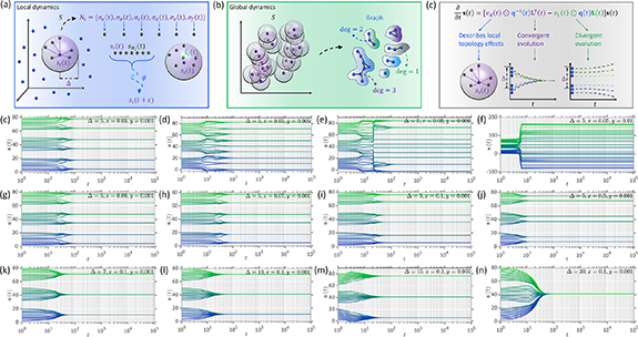
Figure 1. Conceptual illustrations of the Laplacian dynamics of convergent and divergent collective behaviors and the computational experiments with regular initialization. (a) On a local scale, the dynamics of each unit is determined by the interactions between it and its neighbors. (b) Based on the underlying graph structure, the local dynamics of every unit can be related to the global dynamics. (c) The joint dynamics on a global scale is shaped by local topology effects, the tendencies of convergent evolution, and the tendencies of divergent evolution. (d)–(l) The results of computational experiments with regular initialization and different parameter settings are visualized. A homogeneous system with uniform motions is defined on 30 units, whose states are defined as 1-dimensional to offer a clear vision. In the regular initialization, these units are divided equally into 3 groups. The distance between units within each group is set as 2 and the distance between adjacent groups is set as 10. The experiments run 105 iterations under each condition.
Download figure:
Standard image High-resolution imageThe localization of interaction rules is realized by constraining Ni , the neighbor set of unit σi , as a sub-set of units whose states are close to σi

where  denotes an arbitrary distance function and Δ is a parameter that determines the interaction range (see figure 1(a)). Please note that set Ni
evolves across time according to equation (2) as the unit state is time-dependent.
denotes an arbitrary distance function and Δ is a parameter that determines the interaction range (see figure 1(a)). Please note that set Ni
evolves across time according to equation (2) as the unit state is time-dependent.
A convergent evolution process is defined as a global pattern of the system, during which units become increasingly similar to each other in the state space. This process also corresponds to the case where the states of all units approach the global mean state. The non-triviality of this process lies in that each unit only interacts with its neighbors and, consequently, can never know the absolute coordinates of all units in the state space. Only the relative coordinate information obtained through interactions is available for units at each moment. For each unit σi , the relative coordinate of each of its neighbors in the state space is defined as

Given this information, unit σi can only approach the time-dependent local mean state

during convergent evolution. Note that  in the denominator of equation (4) is used to deal with the case with
  .
.
The above definitions have described the convergent evolution process of collective behaviors on a local scale. To study its non-trivial manifestation on a global scale, we need to relate equation (4) with specific global characteristics of the system.
3. Global dynamics of convergent evolution
We notice that equation (4) can be equivalently reformulated as

where  denotes the time-dependent adjacency matrix

In equation (6), notion  denotes the Kronecker delta function and
  is the Heaviside step function. By simple calculation, we can transform equation (4) as
where  denotes the degree in a graph defined by the adjacency matrix in equation (6).
If we consider the observable global state

where  denotes the transpose, we can reformulate equation (7) into a new form

based on vector 

We notice that vector  in equation (9) happens to coincide with the ith row of the degree matrix in graph theory, where the ith entity is the degree of unit i at moment t while all other entities are zeros. Meanwhile, vector
 ![$\left[\mathbf{A}_{i1}\left(t\right),\ldots,\mathbf{A}_{i\vert V\vert}\left(t\right)\right]$](https://content.cld.iop.org/journals/2632-072X/4/2/025013/revision2/jpcomplexacd6cbieqn17.gif) in equation (9) is known as the ith row of the time-dependent adjacency matrix. These observations remind us that
in equation (9) is known as the ith row of the time-dependent adjacency matrix. These observations remind us that ![$\left[\mathbf{A}_{i1}\left(t\right),\ldots,\mathbf{A}_{i\vert V\vert}\left(t\right)\right]-\mathbf{d}_{i}\left(t\right)$](https://content.cld.iop.org/journals/2632-072X/4/2/025013/revision2/jpcomplexacd6cbieqn18.gif) is actually the ith row of matrix
is actually the ith row of matrix  , where
  is the time-dependent Laplacian of the corresponding graph

Taken together, the ith row of the time-dependent Laplacian  can be naturally discovered in the formulation of dynamics when we analyze the state of unit i.
Given the above foundation, we can analyze the observable global state of the system in equation (8) applying the time-dependent Laplacian. Specifically, after defining the observable of all local mean states

and the observable of the inverse of the degrees of all units

using the diagonal  , we can eventually derive a global version of equation (4)

Please see figure 1(b) for illustrations. Equation (14) describes the states of all units in a unified manner while equation (9) serves as a special case of equation (14) where only the state of unit i is analyzed.
Now, let us consider the global dynamics characterized by equation (14). We define an abstract velocity matrix to quantify the intrinsic degrees of the willingness of units to exhibit convergent evolution in the state space

where 1 denotes an all-one row vector of an appropriate size that is applied to ensure the consistency of matrix dimensions. Under the assumption of time continuity, the dynamics for  to approach
  during convergent evolution is formalized as

where local topology effects are described by  (i.e. how the neighbors of a unit affect its evolution), and
  denotes the Schur product (or referred to as the element-wise product between matrices, i.e. we have
  if
if  for arbitrary matrices X, Y, and Z of the same size). In equation (16), the time-dependent Laplacian
  serves as a bridge to make the dynamic evolution of global system states incorporate with the local interactions among units described by graph topology.
4. Global dynamics of divergent evolution
Then we turn to analyze the divergent evolution processes of collective behaviors. At the first glance, one only needs to consider the intrinsic degrees of the willingness of units to exhibit divergent evolution

and assume that units depart from associated time-dependent local mean states by moving in a direction opposite to equation (16). Under this condition, the joint dynamics of convergent and divergent evolution is nothing more than a Newtonian motion in the state space, ![$\frac{\partial}{\partial t}\mathbf{s}\left(t\right) = -\left[\mathbf{v}_{\textrm c}\left(t\right)-\mathbf{v}_{\textrm d}\left(t\right)\right]\odot\mathbf{q}\left(t\right)\mathbf{L}\left(t\right)\mathbf{s}\left(t\right)$](https://content.cld.iop.org/journals/2632-072X/4/2/025013/revision2/jpcomplexacd6cbieqn30.gif) .
.
However, it is unreasonable for our framework to be so trivial because Newtonian mechanics may be impractical in the abstract state space. The information of the mentioned opposite direction can be unavailable in real cases. For instance, if the state space describes the preference of drinks, it is impossible to precisely define an opposite direction of preferring coffee, i.e. it is difficult for units to tell preferring which drink is opposite to preferring coffee. This is because the definition of an opposite drink of coffee is ill-posed, at least in most situations. To describe these non-negligible cases where Newtonian mechanics is unacceptable, we need to consider a weaker assumption.
Our idea arises from the relation between  and
and  , where
  denotes the Moore–Penrose pseudoinverse [34]. To understand their relation, let us consider an instance where the covariance matrix units is defined as
  . Two units are expected to evolve inversely (i.e. they have a negative covariance) if they are connected by an edge in the graph defined by equation (6). In this case, adjusting edges is equivalent to adjusting the differences (i.e. gradients) between units. Therefore, equation (16) can utilize
  in the derivative to minimize those differences. If we further consider the associate precision matrix
  , we can relate the partial correlation [35, 36] between units σi
and σj
with
, we can relate the partial correlation [35, 36] between units σi
and σj
with 

Based on equation (19), two units are expected to evolve consistently (i.e. have a positive partial correlation) if they correspond to a negative value in  (i.e. a positive value in
  ). In this case, adjusting edges is equivalent to controlling similarities between units. During divergent evolution, units are expected to minimize their similarities, which can be realized by the term
  in the derivative of the following dynamics

In equation (20), we use  , the inverse matrix of
  , to characterize local topology effects.
5. Joint global dynamics of convergent and divergent evolution
Now, we have the opportunity to define the joint global dynamics of convergent and divergent evolution based on equations (16) and (20). Specifically, the joint dynamics is given as

which is essentially a type of generalized Laplacian dynamics with more complicated details (see [37–39] for the elementary Laplacian dynamics). See figure 1(c) for illustrations. Although the idea underlying equation (21) is natural and simple, analyzing the dynamic properties of equation (21) is intricate because the competition between convergent and divergent evolution is characterized by the non-trivial interaction between  and
and  under the effects of local topology. To offer a clear vision, we primarily consider a special case of equation (21) in our subsequent analysis.
6. A special case on a homogeneous system with uniform motions
The considered special case of equation (21) is a homogeneous system of units that exhibits uniform motions in the state space. To create uniform motions (i.e. with constant velocities) and make the system homogeneous (here, being homogeneous refers to the case where all units share the same intrinsic properties), we need to define


where  are specific constants that we can manipulate (e.g. used as controlling factors). Equations (22) and (23) make all units share the same and uniform intrinsic willingness degrees, x or y, to exhibit convergent or divergent evolution.
Therefore, in a homogeneous system with uniform motions, equation (21) reduces to a simple form


which is easier to analyze. In computational experiments, we apply the following numerical iteration

to derive the results of equation (25). Note that equation (26) only serves as a simple illustration. One can also consider more complicated numerical approaches.
For the sake of visualization, we mainly consider a 1-dimensional state space in our work, yet a state space with higher dimensions can be directly analyzed without any modification. In figures 1(d)–(l), we present diverse instances of this homogeneous system with different parameter settings, where a regular initialization condition of the system is applied to offer a clear vision (i.e. initialized units are uniformly distributed and form clear cluster structures in the state space). As shown in figures 1(d)–(i), different ratios between x and y in equation (24), i.e. different ratios between the intrinsic willingness degrees of convergent and divergent evolution, create distinct trends of collective behaviors. A larger x can lead to convergent evolution while a larger y makes units divergent. As suggested by figures 1(j)–(l), the change of local interaction range controlled by a varying Δ in equation (2) leads to distinct final patterns in the state space after evolution. A larger local interaction range can amplify the trends of convergent and divergent evolution because more units are involved. These phenomena can also be observed in figure 2, where a random initialization condition is applied to the system (i.e. the initial states of units are randomly sampled following a specific distribution). These results provide qualitative illustrations of the global dynamics of collective behaviors and suggest how the dynamics is shaped by the competition between convergent and divergent evolution trends or by the local interaction range.

Figure 2. The computational experiments with random initialization. (a)–(c) The results of the computational experiments are derived based on a homogeneous system of 30 units with uniform motions in a 1-dimensional state space. In the random initialization, each unit is assigned with an initial coordinate in the state space that is randomly selected following a uniform distribution in ![$\left[0,100\right]$](https://content.cld.iop.org/journals/2632-072X/4/2/025013/revision2/jpcomplexacd6cbieqn46.gif) . The experiments run 105 iterations under each condition.
. The experiments run 105 iterations under each condition.
Download figure:
Standard image High-resolution imageTo quantitatively analyze the convergent and divergent evolution of collective behaviors, we study the properties of the eigenvalue spectrum of  . Specifically, we analyze the standardized moments of the eigenvalue spectrum to reflect the latent dynamics of the evolution process (note that the first and the second standardized moment are not considered because they are constant [40]). Meanwhile, we consider
  , the distance between state
  and its k-nearest state at moment t given a distance function
  in equation (2). We define the average k-nearest distance at moment t as

to characterize the global state of the system at moment t. In figure 3, these two kinds of metrics are calculated on three representative instances of the homogeneous system in equation (25). As shown in figure 3, distance  exhibits distinct changes during convergent and divergent evolution (we define
  as the Euclidean distance for convenience). Before the dynamics converges to its limit, the standardized moments of the eigenvalue spectrum dramatically increase during divergent evolution while decreasing during divergent evolution.

Figure 3. The eigenvalue spectrum of matrix  and the average k-distance in state space. (a)–(c) The observable of matrix
  is derived using the homogeneous systems generated in figures 1(f), (l) and 2(b), where we measure the mth standardized moments of the eigenvalue spectrum. The measured results of
  are marked by colors, where the color changes from blue to green as m increases. (d)–(f) The average k-distances in state space, where
  , are measured as the functions of time. The color changes from blue to green as k increases.
Download figure:
Standard image High-resolution imageThe results shown in figure 3 inspire us to distinguish between convergent and divergent phases using  , the relative ratio between the average k-nearest distances at moment 0 and moment t. This ratio is larger than one in the divergent phase while it is smaller than one in the convergent phase. In figure 4, we analyze the phase space of the homogeneous system in terms of
  under different conditions of x, y, and Δ. As shown in figures 4(a)–(f), convergent and divergent phases share a non-trivial and relatively blurry boundary on the plane of
  , which changes across different local interaction range conditions. Phase-transition-like phenomena can be observed if we consider
  as an order parameter and treat the ratio between the intrinsic willingness degrees of convergent and divergent evolution in equation (24),
  , as a control parameter in figures 4(g)–(l). A kind of phase-transition-like processes from the divergent phase to the convergent phase can be observed as
  increases, during which the collective behaviors of units experiences drastic changes. Specifically, before
  reaches a certain value, all units generally exhibit divergent evolution. In this phase, units tend to be further away from their neighbors as time goes by (i.e. become increasingly different). After
  exceeds a specific threshold, units change to exhibit convergent evolution. In this phase, units have stronger tendencies to approach to their neighbors in the state space (i.e. become increasingly similar).

Figure 4. The phase space of convergent and divergent evolution. (a)–(f) Given each condition of  , we generate a homogeneous system with uniform motions and regular initialization for every
 ![$\left(x,y\right)\in\left[0.001,0.2\right]^{2}$](https://content.cld.iop.org/journals/2632-072X/4/2/025013/revision2/jpcomplexacd6cbieqn58.gif) and run the experiment for 105 iterations. The generated results support the measurement of ratio
and run the experiment for 105 iterations. The generated results support the measurement of ratio  (k = 3). The heat maps of this ratio under all conditions are shown in (a)–(f), where different color maps are used to distinguish between different settings of Δ. (g)–(l) Ratio
  is shown as a function of
  under each experiment condition, where color maps are consistent with (a)–(f).
Download figure:
Standard image High-resolution imageHere we emphasize that these processes should be treated as phase-transition-like phenomena rather than strict phase transitions. It remains elusive whether these phenomena really arise from specific underlying phase transitions or from other unknown mechanisms with similar appearances. Diverse theoretical difficulties are met when we attempt to confirm the detailed properties of these phase-transition-like phenomena (e.g. the order of transition and scaling relation), which impede us from verifying the potential existence of the phase transition. Therefore, the existence of potential phase transition in the Laplacian dynamics of convergent and divergent collective behaviors remains as a hypothesis. Below, we summarize the main difficulties of studying this conjecture.
7. Mathematical challenges for studying homogeneous system with uniform motions
The main challenges for studying the observed phase-transition-like phenomena arise from the non-triviality of predicting the limiting behaviors of the homogeneous system (i.e. the classification of convergent and divergent phases depends on the limit state of the system after the evolution process converges).
Although the motions of units in the state space have been constrained as uniform, the homogeneous system in equation (25) is shaped by complicated local topology effects, which is in contrast to a more theoretically favorable case where local topology effects are completely excluded

In such an ideal case, we have the opportunity to express  , the eigenvalues of matrix
  , based on the eigenvalues
  of matrix

Meanwhile, matrix  shares the same group of eigenvectors,
  , as matrix
  . Equation (29) is derived from the fact that the eigenvalues and eigenvectors of matrix
  are
are  and
and  , respectively [41, 42]. The explicit eigen-decomposition of
  provides rich information about the evolution dynamics, making it possible to analyze equation (28) following the dynamic system theory [42]. However, this possibility vanishes due to the local topology effects in equation (25). To quantify these non-trivial effects, we can measure the cosine distance between the vector of eigenvalues of
  and that of
  (similarly, between the vector of eigenvalues of
  and that of
  ). Meanwhile, we can calculate the average cosine distance between the eigenvectors of
  and those of
  (similarly, between the eigenvectors of
  and those of
  ). These cosine distances reflect the local topology effects on the eigenvalues and eigenvectors of
  and
and  . In figures 5(a) and (b), we present an instance calculated on a representative homogeneous system, suggesting that these non-negligible local topology effects are volatile until the evolution dynamics converges. Therefore, equation (29) departs from the actual properties of equation (25) in most cases.

Figure 5. The non-trivial properties of the Laplacian dynamics of convergent and divergent collective behaviors. (a), (b) The local topology effects (LTE) on the eigenvalues and eigenvectors of  and
and  are shown as the functions of t based on the homogeneous system generated in figure 1(l) (also see the inserted sub-plot in figure (c)). (c) The deviation of
  from being commutative is measured by the proposed commutator error (CE), where the applied homogeneous system is shown in the inserted sub-plot for reference.
Download figure:
Standard image High-resolution image
Moreover, another challenge arises from that  in equation (25) is not commutative until the evolution dynamics converges to its limit. We can measure the deviation of
  from being commutative based on

where ![$\left[\cdot,\cdot\right]$](https://content.cld.iop.org/journals/2632-072X/4/2/025013/revision2/jpcomplexacd6cbieqn96.gif) denotes the commutator and
denotes the commutator and ![$\left[\cdot,\cdot\right]_{ij}$](https://content.cld.iop.org/journals/2632-072X/4/2/025013/revision2/jpcomplexacd6cbieqn97.gif) is the
is the  th element of the commutator. We refer to
  as the commutator error. In figure 5(c), we calculate an instance of
  by setting
  . The derived results suggest that
  becomes trivially commutative only after it arrives at its limit. The absence of a commutative
  in most cases makes it invalid to express the solution of equation (25) as
  , rejecting the possibility of simplifying equation (25).
In sum, the above properties create obstacles for theoretically analyzing the homogeneous system in equation (25). The situation becomes even more non-trivial if we relax the constraints on  and
and  to consider heterogeneous cases. These challenges may serve as valuable directions for future theoretical studies.
8. Discussion
In this study, we propose a minimal model to describe the convergent and divergent evolution of collective behaviors. Despite its mathematical simplicity, the model exhibits abundant non-trivial behaviors and suggests the potential existences of phase-transition-like phenomena between convergent and divergent evolution controlled by local interactions. The non-triviality of the proposed model may inspire new mathematical techniques in analyzing the physics of collective dynamics. Moreover, the simplicity of the proposed model in computational aspects enables it to serve as a foundation for developing large-scale numerical simulations of collective behaviors.
While the current work primarily focuses on the theoretical analysis of the proposed model, more explorations in model applications can be considered in future studies. The proposed model may find its place in studying the social dynamics of people and animals [1, 2, 8] (note that numerous animals, such as chimpanzees, have complex social behaviors). For instance, the state space can be used to describe opinions, where the Newtonian mechanics may be not applicable (i.e. opinions are usually vague and do not support a precise definition of the opposite direction) [8]. The Laplacian dynamics of convergent and divergent evolution of opinions can be used to model the emergence and collapse of consensus in social networks. In the divergent phase, units tend to differentiate their opinions to improve the uniqueness of their attitudes. In the convergent phase, units attempt to forge consensus and form a certain number of clusters where each cluster of units share a representative opinion. In somewhere between these two phases, units may seek common points while reserving differences in their opinions. In general cases where the intrinsic willingness degrees of convergent or divergent evolution are not constrained as homogeneous and constant but are allowed to vary (e.g. let  and
and  change across time or be correlated with unit states), the proposed model may be able to reproduce the intricate evolution of public opinions. A possible way to relate our model with existing models in opinion dynamics is to make
  and
and  time-dependent and correlated with the size of the neighbor set. As an illustration, one can let
  or
or  be positively correlated with
  for every unit σi
. Under this condition, the actual velocity of convergent or divergent evolution of a unit critically depends on the size of cluster where this unit belongs to, making it possible to describe social impacts (e.g. how convincing power depends on the size of social groups [8]) by our model. To this aim, one can apply our framework to study the opinion dynamics characterized by diverse classic models. In the case where opinions are discrete, one can discretize the state space and apply our model to study the cellular automata developed by Latané [43] and Nowak et al [44], whose statistical mechanics has been previously analyzed at the mean-field limit [45] but remains elusive in more general cases. Given the extensive applications of this cellular automata and its variants in studying social opinions [43, 44], learning [46], the effects of leaders on opinion formation [47–49], and the mitigation of social impacts due to population diversity [50] (see [51] for a review), our model may serve as an alternative choice for formalizing these collective behaviors apart from the mean-filed approximation. Except for the cellular automata mentioned above, the Sznajd dynamics [52–57] can also be analyzed applying our model, which suggests the possibility for our model to be used in studying opinion spreading under social impacts [52–54], voting [58], and the interaction of economics and opinions [54]. In the case where opinions are continuous, our model can also be defined on the dynamics generated by the Deffuant model [59], the Hegselmann–Krause model [60], and their density-based variants (see [61] for a review). In these models, an assumption referred to as the bounded confidence is applied, implying that units only have effective interactions with peers with similar opinions [61]. When the differences between opinions are not tolerable, interactions become non-effective [61]. This property can be naturally and equivalently described by the local interaction rule in our model. Apart from opinion dynamics, other topics in social dynamics (see a summary in [8]) may also be analyzed by our model, which remains for future explorations.
for every unit σi
. Under this condition, the actual velocity of convergent or divergent evolution of a unit critically depends on the size of cluster where this unit belongs to, making it possible to describe social impacts (e.g. how convincing power depends on the size of social groups [8]) by our model. To this aim, one can apply our framework to study the opinion dynamics characterized by diverse classic models. In the case where opinions are discrete, one can discretize the state space and apply our model to study the cellular automata developed by Latané [43] and Nowak et al [44], whose statistical mechanics has been previously analyzed at the mean-field limit [45] but remains elusive in more general cases. Given the extensive applications of this cellular automata and its variants in studying social opinions [43, 44], learning [46], the effects of leaders on opinion formation [47–49], and the mitigation of social impacts due to population diversity [50] (see [51] for a review), our model may serve as an alternative choice for formalizing these collective behaviors apart from the mean-filed approximation. Except for the cellular automata mentioned above, the Sznajd dynamics [52–57] can also be analyzed applying our model, which suggests the possibility for our model to be used in studying opinion spreading under social impacts [52–54], voting [58], and the interaction of economics and opinions [54]. In the case where opinions are continuous, our model can also be defined on the dynamics generated by the Deffuant model [59], the Hegselmann–Krause model [60], and their density-based variants (see [61] for a review). In these models, an assumption referred to as the bounded confidence is applied, implying that units only have effective interactions with peers with similar opinions [61]. When the differences between opinions are not tolerable, interactions become non-effective [61]. This property can be naturally and equivalently described by the local interaction rule in our model. Apart from opinion dynamics, other topics in social dynamics (see a summary in [8]) may also be analyzed by our model, which remains for future explorations.
Acknowledgments
This project is supported by the Artificial and General Intelligence Research Program of Guo Qiang Research Institute at Tsinghua University (2020GQG1017) as well as the Tsinghua University Initiative Scientific Research Program.
Data availability statement
All data that support the findings of this study are included within the article (and any supplementary files).