
A measured data correlation-based strain estimation technique for building structures using convolutional neural network
Abstract
A machine learning-based strain estimation method for structural members in a building is presented The relationship between the strain responses of structural members is determined using a convolutional neural network (CNN) For accurate strain estimation, correlation analysis is introduced to select the optimal CNN model among responses from multiple structural members. The optimal CNN model trained using the response of the structural member with a high degree of correlation with the response of the target structural member is utilized to estimate the strain of the target structural member The proposed correlation-based technique can also provide the next best CNN model in case of defects in the sensors used to construct the optimal CNN. Validity is examined through the application of the presented technique to a numerical study on a three-dimensional steel structure and an experimental study on a steel frame specimen.
1.Introduction
When subjected to strong loads associated with natural disasters that exceed the load levels considered in the design phase the structure suffers unexpected damage. If damage occurs to some components, the structure loses its expected structural function, undergoes greater damage due to the additional load, and may eventually collapse. Such damage may cause serious economic losses and result in casualties [1, 2]. Therefore, continuous building monitoring and maintenance are required to ensure the safety of a building structure. In this regard, structural health monitoring (SHM) techniques have been developed to identify structural behaviors and evaluate safety with precision [3, 4, 5]. In the SHM fields, various structural responses such as displacement, acceleration and strain are measured using sensors installed in the structure [6, 7, 8]. Structural health is currently evaluated based on the analysis of the measured structural response. The lateral displacement of a high-rise building can be measured using a device for displacement measurement with GPS, while the safety of a high-rise building is assessed via measured displacement under wind loads [10, 11, 12, 13]. Vibration in buildings can be measured using accelerometers attached to multiple floors of the building. Aside from the vibration under strong loads, the vibration under ambient excitation is also measured to determine the dynamic characteristics of a building structure, through which the building status can be evaluated [10, 11, 12, 13]. Strain sensors have been used in buildings to more directly evaluate the safety of structural members such as columns, beams and walls [14]. The stress of the members can be obtained from the measured strain response of the structural member, which can then be used to evaluate safety [15].
Various types of strain sensors such as long gage fiber optic sensor [6, 17], vibrating wire strain gage [18] and fiber Bragg grating sensors [19] have been developed and applied in structural safety assessment In the initial stage of their use after a building’s completion, strain measurement can be done without any complication, and the stress of the structural member can be evaluated based on the results. However, with the current technology, long-term structural health monitoring is difficult because the lifespan of the sensor is significantly shorter than that of the building [20]. There may be instances when it is not feasible to measure structural responses due to a temporary or permanent failure of the sensor during the monitoring process. Displacement and acceleration sensors can be replaced in case of a failure, but this is not possible with strain sensors, which are embedded in concrete. The strain sensor installed on the surface of a structural member can be replaced, but a newly installed strain sensor cannot reflect the stress that has already occurred in the structural member. In this case, the measured value may not be representative of the actual strain value of the structural member. Transmission of information on structural responses measured from the sensor attached to the structural member is generally done using a wireless communication system [21, 22]. In this case, the measured structural strain response may be lost due to problems with data transmission and temporary power supply [23, 24].
In response to situations where strain sensing is impossible or when strain data is lost, techniques for strain data prediction and recovery have been developed based on the measured strain response data in advance. Several researchers have proposed strain response prediction methods using correlation among strain responses measured from installed strain sensors. Chen et al. [25] utilized the correlation between the sensors for strain data recovery Using the nonparametric copulas technique, they investigated the interdependence between the response of the strain sensor installed at one location and the structural strain response measured from the sensor installed at another location which was then applied to predicting the lost strain response. Zhang and Luo [26] presented a technique for missing stress data recovery based on the correlation between the measured stress data. Using the regression technique, they analyzed and identified the correlation between multiple measurement points, through which they recovered the missing stress data of the steel structure. Skafte et al. [27] proposed a time history strain estimation method based on operational modal analysis. The vibration responses measured from structures, such as the acceleration response, are divided into high and low frequency parts. The high frequency part is decomposed into the modal coordinate and then strain responses are extracted by multiplying the modal coordinate with the strain mode shape. The low frequency part of the strain response is decomposed by Ritz-vectors, which are then are extracted from the finite element model by employing a load. Strain responses for low frequency are subsequently derived by multiplying the decomposed data with the strain Ritz-vector. The strain time history response was finally obtained by summing the strain responses corresponding to the two parts. The proposed method was applied to estimate the strain in an offshore structure. Bharadwaj et al. [28] presented a time history of strain response prediction technique using strain mode shapes obtained through highspeed image capture. The limited response measured using the strain sensor is expanded by the strain mode shape and is used to extract the full-field strain. The proposed technique was verified through time history strain response prediction of a composite spoiler. Wang and Ni [29] proposed a Bayesian modeling approach, which can probabilistically predict the dynamic strain response of a structure. The proposed Bayesian dynamic linear model predicts both stationary and non-stationary time history strain responses. The time-dependent strain response is also predicted by reflecting the long-term trend and seasonal change in the strain response to the proposed technique. The applicability of the proposed technique was examined using the strain response collected from an actual structure which is a cable-stayed bridge.
Machine learning techniques have been applied to various researches on data estimation and prediction [30, 31, 32, 33]. Those techniques have also been introduced to predict and recover strain data [34, 35]. Kromanis and Kripakaran [36] introduced a support vector machine (SVM) for long-term strain prediction of structures. The SVM was used to investigate the relationship between the temperature and temperature-induced strain response of concrete structures and predict the strain response using the relationship. A convolutional neural network (CNN) that not only facilitates processing big data because it hardly requires handcrafted work of input data, but also has high-accuracy prediction, recognition and classification performance [37, 38, 39, 40, 41], has been introduced recently in strain estimation research. With this development, studies intended to determine the correlation between strain and structural responses other than strain with CNN have been undertaken for strain estimation and recovery Gulgec et al. [42] presented a deep learning-based strain sensing technique by combining data measured using an accelerometer In the proposed technique, the collected acceleration response was set as input information of a deep neural network using long short-term memory and fully connected layers in order to estimate the time history of strain response. The strain sensing performance of the proposed technique was evaluated using the structural response measured from a steel beam-like structure for a relatively long period. Chen et al. [43] presented a long-term strain reconstruction method. In the method, a nonlinear deep learning model was employed to capture the long-term and short-term pattern of strain responses. In the deep learning model, strain data from one sensor, temperature data from one sensor, and air temperature data were set in the input and the target response is set as strain data from another strain sensor. The presented method was validated by using long-term measured data from a structure and reconstruction performances of the results were evaluated for multiple sensing scenarios.
This study presents a strain estimation technique for building structures based on correlation analysis. In the proposed technique, CNN, one of the machine learning techniques, is used to determine the relationship of strain responses of the structural members. The strain responses of adjacent members and ground acceleration are set as the CNN input, while the strain responses of target structural members subject to safety assessment are set as the CNN output. The CNN trained using the measured structural response data estimates the strain response of the target structural member. For accurate and efficient strain response prediction of the target structural member, the correlation analysis of measurement data from multiple strain sensors installed in the building’s structural members is introduced prior to CNN training. In the technique, Pearson correlation analysis is employed to select an optimal CNN The proposed strain estimation technique is applied to a numerical study on the American Society of Civil Engineers (ASCE) benchmark model and an experimental study with a shaking table test on a 3-story steel frame specimen Through application, the strain estimation performance of the optimal CNN model searched via the proposed technique is examined. The adequacy of the data types in the input map configuration of the proposed CNN is also investigated. In addition, the effectiveness of a method for selecting the optimal CNN based on the correlation analysis in the proposed technique is then verified. Strain estimation performance according to variations in input size in the CNN architecture is consequently confirmed.
The main contribution of the presented technique lies in the selection of the optimal CNN for estimating strain responses of the target member in a reasonable manner. To find the adjacent structural members representing the highest correlation with the target member, the correlation analysis of measured responses between adjacent and target members is employed. Through the correlation analysis, the adjacent members are found and their responses are used to train the optimal CNN model with the most accurate strain estimation performance. In addition, considering the defect of the sensors in the structural members, the prior correlation analysis results can also provide the next best CNN model. Using the alternative CNN model, the strain responses can be estimated with relatively high accuracy in a stable and prompt manner in case any defect in the sensors installed in the already identified adjacent members is found.
2.Methodology
The basic concept of the proposed strain estimation technique is based on the assumption that a structural member has a relationship with adjacent structural members in terms of the response to loading. To identify the relationship, the correlation between a specific structural member and many adjacent structural members is investigated. Through the established correlational relationship, the responses of multiple adjacent structural members are also used to estimate strain responses of specific target structural members.
The structural response relationship between a target structural member and adjacent members is made through the CNN, which is one of the machine learning techniques. Because there are numerous structural members, many CNNs can be formed to represent the relationships with many adjacent members to estimate the strain in a specific structural member Using the measured structural response subjected to various excitations, the CNN is trained to establish the relationship between structural members.
Figure 1.
Framework of the proposed approach.
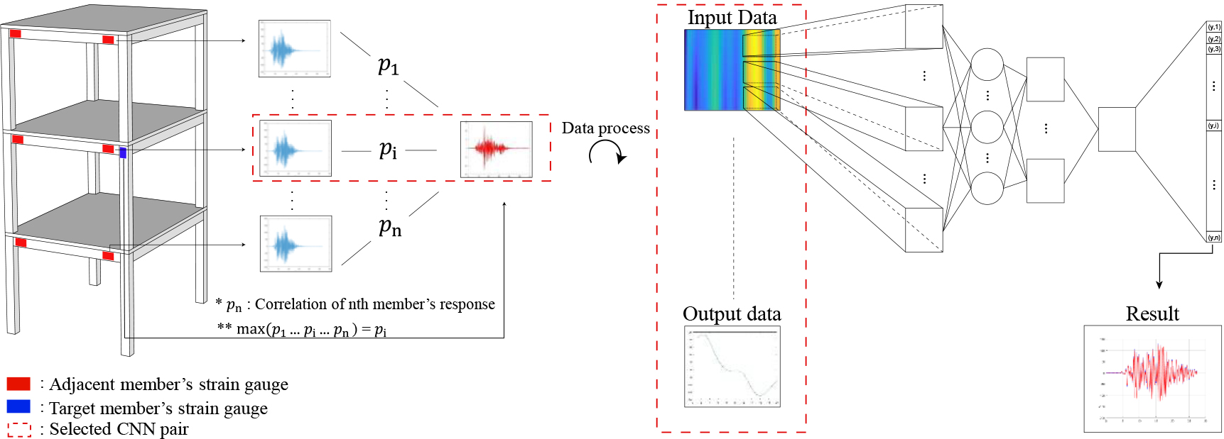
Although there are various types of relationships established between the structural response of a target structural member and the response of many adjacent structural members, there will be specific adjacent structural members that are most closely related to the structural response of the target structural member (member A). Accordingly, it is necessary to select a CNN with the closest correlation with the target member (member A) among many CNNs built between the target member (member A) and many adjacent members for more efficient strain response estimation. Thus, this technique includes the correlation-based selection of an optimal CNN for the strain estimation of the target member.
The CNN of the adjacent member that is most effective and has the closest correlation for estimating the strain response of a specific member is selected in this technique. To select the CNN, a correlation analysis between the measured structural response data of the target structural member and adjacent members is conducted. Based on the correlation analysis, the CNN between the target member and the adjacent member with the highest correlation is selected and adopted as the optimal CNN for use in estimating the strain response of the target member.
If there is a change in the monitoring system due to defective sensors, it may be impossible to use the optimal CNN based on the correlation. In this case, except for the defective CNN among many CNNs between the target structural member and many adjacent structural members, the next best CNN can be derived from the correlation analysis. This alternative CNN is employed to reliably estimate strain responses of the target structural member. The framework for the proposed approach is shown in Fig. 1.
2.1Structural response estimation using CNNs
In the proposed strain estimation technique, the relationship between the structural responses of the target structural member and many adjacent structures is determined by the CNN Consequently, many CNNs can be trained according to the number of members adjacent to the target member In this study, the strain response that can directly evaluate the safety of structural members was selected as the target structural response. The target load was also limited to seismic load, which is one of the dynamic loads that can cause serious damage to structures.
Table 1
Detailed information on the CNN layer and operator
| Layer | Size/Depth | Operator | Size |
|---|---|---|---|
| Input layer | 20 | Kernel 1 | 9 |
| Convolutional layer 1 | 12 | Subsampling 1 | 2 |
| Pooling layer 1 | 6 | Kernel 2 | 5 |
| Convolutional layer 2 | 2 | Subsampling 2 | 1 |
| Pooling layer 2 | 2 | ||
| Fully connected layer | 80 | ||
| Output layer | 20 |
Figure 2.
CNN architecture for strain estimation.
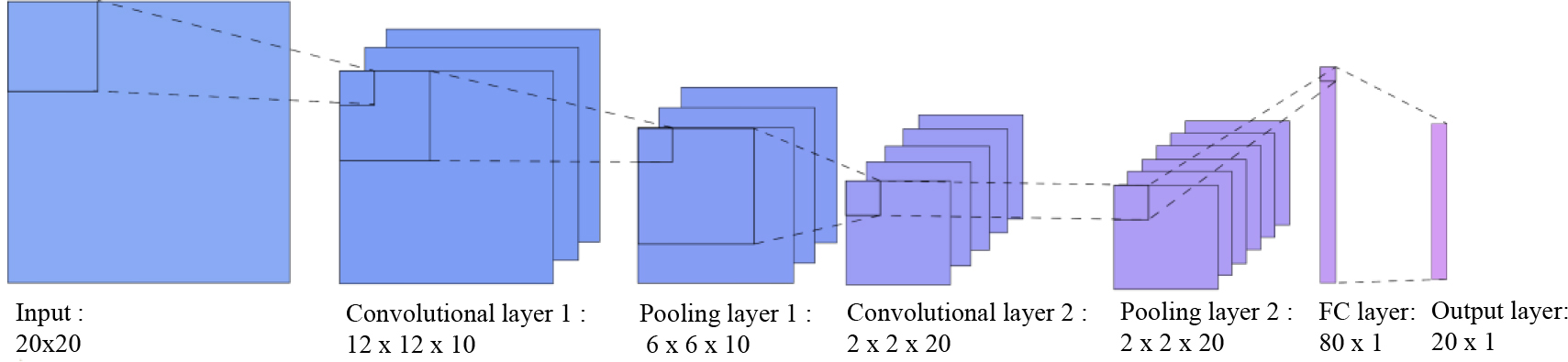
The strain response is measured and accumulated by strain sensors installed on the target structural member to be monitored and adjacent structural members under seismic loading. The obtained strain responses are used to build CNNs representing the relationships between the target member and adjacent members When monitoring of the target member is impossible, the strain of the target member is estimated using a CNN trained with the structural response of the member that is highly correlated with the target member. Accordingly, the strain response of the adjacent structural member highly correlated with the target member is set in the CNN input layer for strain estimation of the proposed technique. The strain response of the target member is set in the CNN output layer. There are two pairs of convolutional and pooling layers between the input layer and the output layer. Detailed information on layers and operators present in these layers are summarized in Table 1. A fully connected layer that exists between the second pooling layer and the output layer connects the two layers. The CNN architecture of the proposed technique with the input and output layers set is shown in Fig. 2 Ground acceleration (GM), which affects all structural members during an earthquake and is easier to measure than structural response, is additionally set in the CNN input layer In Section 3, a comparative analysis of the strain estimation performance of the member subject to monitoring due to the additional use of GM data is presented. To constitute input layer, the time series data of the strain responses of the adjacent structural member with the highest correlation with the target members are rearranged to a matrix form according to the time stamp. The GM time series data o are then rearranged to the matrix following the rearranged time series data of strain of the adjacent member. The remaining parts of the matrix are changed by the number of the adjacent members according to the correlation analysis and those remaining parts are filled by zero padding.
2.2Correlation-based activation strategy for optimal CNN selection
Because there are many structural members in a structure, the number of adjacent structural members that can correlate with the target structural member for monitoring is also significant. Accordingly, a number of CNNs can be formed for one target structural member. For a specific dynamic load, the structural response correlation of one target structural member and adjacent members is very complex depending on the location, size, structural role and service load. A process of finding the structural member most closely related to the target member is needed for accurate structural response prediction of the target structural member and safety assessment.
In this study, finding the most effective CNN among multiple CNNs defining the relationship of responses between the target member and adjacent members is referred to as the optimal CNN selection process. To find the most reliable and effective CNN among CNNs for adjacent members, correlation analysis between the strain response data is performed. Prior to the construction of a CNN, the correlation between the strain response of the target member and the strain response of the adjacent members is analyzed to find the member with the highest degree of correlation. The CNN between the strain response of the identified adjacent member and the strain response of the target member is set as the optimal CNN to estimate the strain in the target member.
In the present technique, the Pearson correlation coefficient method was introduced to analyze the structural response correlation between the target member and adjacent members. The Pearson correlation coefficient is a measure of the degree of linear correlation between two variables, with the correlation coefficient having a value ranging from
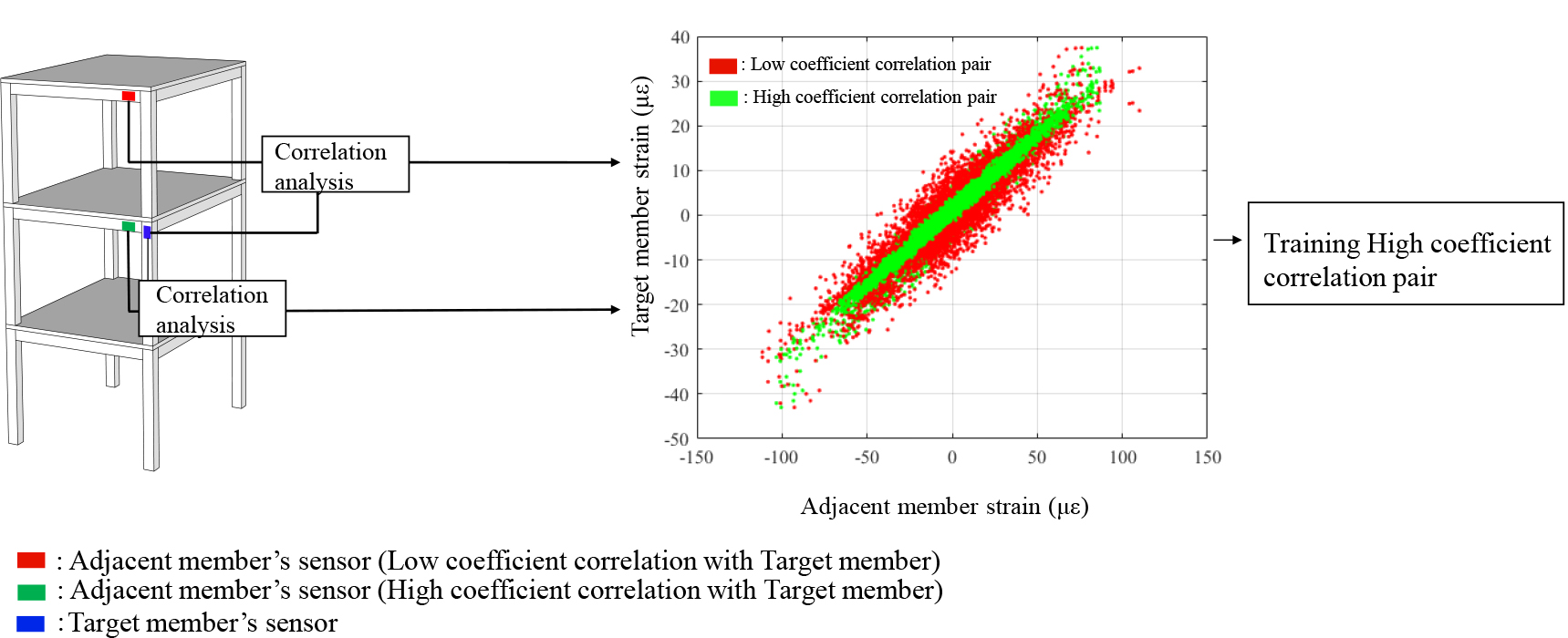
Figure 3.
Correlation coefficient between the target member and adjacent members for the CNN selection.
When the strain response of the target structural member to a specific seismic load is , and the strain response of the
(1)
where
3.Application
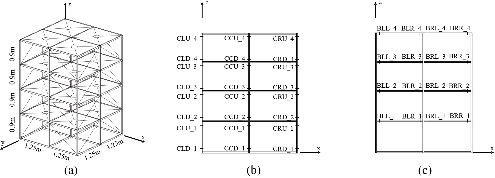
Figure 4.
Example structure (ASCE benchmark model): (a) perspective view; (b) sensor locations in column; and (c) sensor locations in beam.
3.1Numerical study
3.1.1Descriptions on example structure
The ASCE benchmark model was used to examine the effectiveness of the strain estimation technique based on the proposed measurement correlation-based activation strategy. The ASCE benchmark model shown in Fig. 4a is a 4-story 2-span by 2-span steel structure Each story is 0.9 m high, with a total height of 3.6 m and has a plan of 2.5 m by 2.5 m. The cross-sectional dimensions of columns and beams, which are major structural elements for applying the present research technique, are B100
Measurements of the structural strain responses of structural members in the target structure subjected to various earthquakes are needed to apply the proposed technique. In this section, it is assumed that the strain responses extracted through dynamic earthquake analyses on multiple seismic loads have been measured. To this end, the target structure was modeled using OpenSees [46], a nonlinear seismic analysis program, to carry out dynamic analysis of seismic loads. A total of 20 historical earthquakes were selected and used to perform seismic analysis. Detailed information on the earthquakes is given in the literature [47]. As shown in the reference, the structural responses to 18 earthquakes were used to train CNNs to define the relationship between the target member and adjacent members. After training, the structural response estimation performance of the optimal CNN was verified using the structural responses for the test datasets. The test datasets in this application were set as the remaining two earthquakes (19th and 20th earthquakes in the literature [47]) among the 20 earthquakes.
3.1.2Correlation analysis of strain
Figure 5.
Correlation coefficient of strain measurements from the example structure.
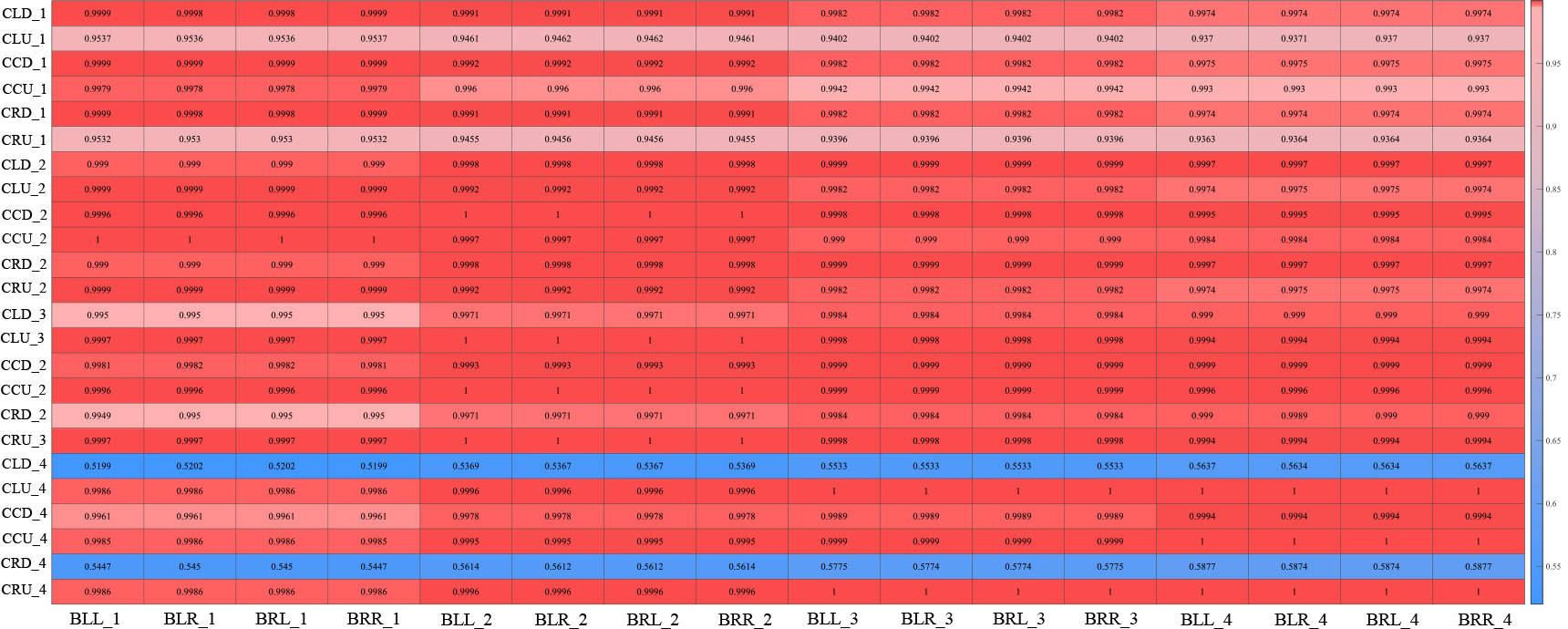
Figure 6.
Training results: (a) convergence curve and (b) comparison of strains between reference and estimated values.

Prior to examining the strain response estimation performance of the proposed technique, correlation analysis for optimal CNN selection was carried out. The structural members subject to monitoring were assumed to be the columns viewed from the side of the benchmark model, and the strain extraction locations where the strain is assumed to be measured in the columns are shown in Fig. 4b. The beam on the same elevation was selected as the adjacent member of the column. The locations of the strain response extraction, where the strain is assumed to be measured in the beam, are shown in Fig. 4c. The specific locations of the columns shown in Fig. 4b correspond to the members subject to monitoring. The correlation coefficients for the strain responses of target members (columns) with those of the beams was calculated using Eq. (1) as shown in Fig. 5. These strain responses to calculate the correlation coefficients were derived from dynamic analysis for the ASCE model subjected to an earthquake load. Using the correlation coefficients, the optimal CNN will be selected and the CNN will be utilized to estimate strain subjected to another earthquake load in the future. It can be confirmed that there is a specific tendency and correlation with adjacent beam members according to the location of the column subject to monitoring (floor, location in the member). For example, the first-floor column showed the highest degree of correlation with the first-floor beam. It was also confirmed that the strain response at the lower end of the second- and third-floor columns had the highest degree of correlation with the response of the second-floor beam. On the other hand, the strain response at the upper end of the second- and third-floor columns was highly correlated with the response of the first-floor beam. The strain response of the fourth-floor column showed the highest degree of correlation with the strain of the fourth-floor beam.
Based on the correlation analysis, it is possible to find the member with the highest degree of correlation using the strain response of the target member subject to monitoring. In this study, the column member is set as the target member. Structures other than the ASCE benchmark model, which have different structural characteristics from the present model, are expected to exhibit different trends from the correlation characteristics analyzed in this study. Therefore, correlation analysis using the strain response measured for each target structure is required for the application of the proposed technique. Although the adjacent member, which has the highest degree of correlation with the target member is selected as the optimal CNN model, training of CNNs to define the relationship between the responses of the other adjacent members and the target member is also needed to avoid unstable strain estimation associated with problems due to sensor failure in the adjacent member corresponding to the optimal CNN.
3.1.3Results of strain estimation
This section examines the strain estimation performance of the proposed technique. The upper part of the central column (CCU_1) on the first floor in Fig. 4b was selected as the structural member subject to monitoring. Accordingly, all beams in Fig. 4b present in the same elevation were selected as adjacent members to be used for the structural response prediction of the target member In addition, 18 earthquakes for training and structural responses were used to train CNNs to define the relationship between the strain responses of the target column member and adjacent beams Among these CNNs, the CNN trained by first-floor beam members (BLL_1 and BRR_1) representing the highest correlation coefficient with the target member was selected as the optimal CNN that exhibits the most accurate strain estimation of the target column member according to the degree of correlation analyzed in Section 3.1.2. Training of the optimal CNN was conducted stably, and this can be confirmed via the convergence curve of the loss function composed of the discrepancy between the CNN estimation output and the labeled data in the output layer during training in Fig. 6a. In addition, Fig. 6b shows the degree of agreement between the reference value and the estimated strain of the optimal CNN for two test earthquakes The trained optimal CNN showed root mean squared errors (RMSEs) of 4.8554 and 4.0656, respectively, for the training and test datasets, and mean squared errors (MSEs) of 2.3106 and 2.9470,
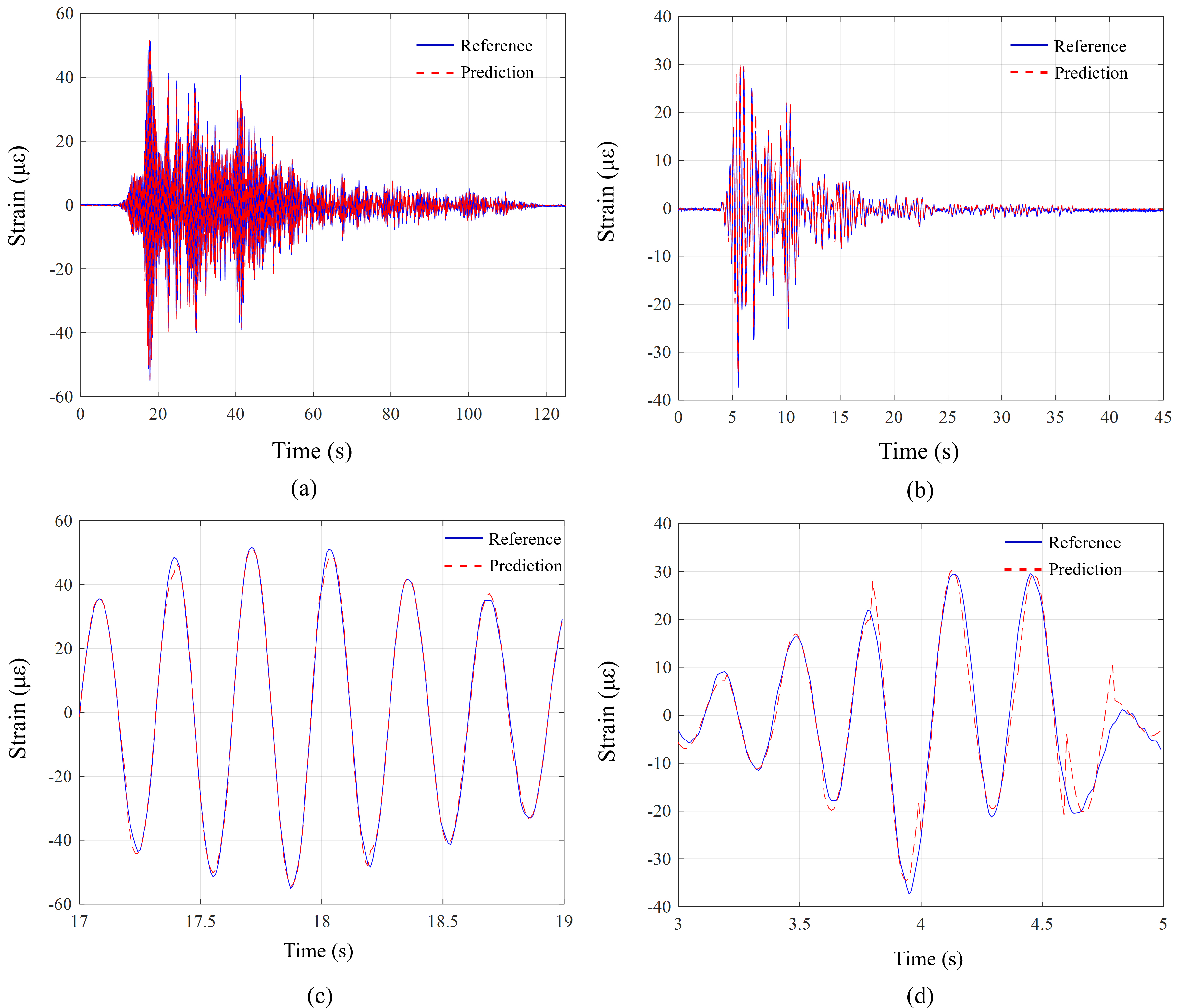
Figure 7.
Strain estimation results subjected to a test earthquake load.
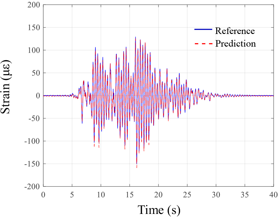
Figure 8.
Strain estimation results: (a) using only GM data and (b) using one beam strain with GM data.
respectively, for the training and test datasets. Figure 6 and error analysis results showed that the proposed technique accurately predicts the strain response of the column subject to monitoring only with the strain response of the adjacent member Fig. 7 shows the strain time history estimation results of the optimal CNN for one test earthquake, which confirmed that considerably accurate response estimation is possible. To investigate the effectiveness of the optimal CNN trained by data with the highest correlation coefficient (0.9979 of CC between CCU_1 and first-floor beam members), the CNNs were additionally trained by data with the lower correlation coefficient and their estimation performances were confirmed. A CNN was trained by data from CLU_1 and first-floor beam members. The correlation coefficient value between them is 0.9537. The CNN trained by data with 0.9537 of correlation coefficient showed RMSEs of 5.7554 and 5.2016. A CNN was additionally trained by data from CLD_4 and first-floor beam members. Their correlation coefficient is 0.5199. In this case with very low value of correlation coefficient, CNN could not be made, which means loss function was not converged during the CNN training. From these results, it is confirmed that the optimal CNN selected by the presented method has excellent estimation performance than other CNNs trained by data with lower correlation coefficients.
As mentioned in Section 2.1, the prediction performance of both the CNN model using the strain of the adjacent members and the CNN model using ground acceleration along with the strain of the adjacent members was analyzed in the CNN input data configuration. The strain estimation performance of the CNN using only ground acceleration data was investigated first. As shown in Fig. 8a if only the GM data is used without the strain of the adjacent member, strain estimation fails with a large RMSE of 47.28. On the other hand, when the GM data and the strain from one measurement location of an adjacent beam member are used together in the CNN input data the RMSE value is 7.36 which indicates that the strain of the target structural member is accurately predicted as shown in Fig. 8b. It can also be confirmed that the RMSE was reduced by 81% compared to the CNN model using only GM data. The above results showed that in applying the present technique, it is difficult to estimate strain of the member subject to monitoring only with the GM data. The strain response of the adjacent member should be used in combination to ensure reliable estimation performance.
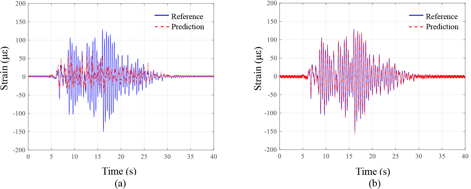
Figure 9.
Influence of GM data in the CNN input on strain estimation performance: (a) by two beam strain data; (b) by two beam strain data with GM data; (c) enlarged plot of (a); and (d) enlarged plot of (b).
This study investigated the influence of GM data added to the optimal CNN model on the strain estimation performance. Figure 9a shows the strain estimation results of the CNN trained using only the strain response of adjacent members as CNN input data, which is the same as in Fig. 7. Figure 9b shows the strain estimation results of the CNN trained using GM data in addition to the strain responses of the adjacent member to the CNN input data. Both predictions were found to estimate the strain response of the target column member with high accuracy and the difference is not significant When GM data was additionally used as shown in Fig. 9b, RMSE for the test dataset was 3.7853, which was about 6.89% lower in RMSE, compared to the case where GM data was not used as in Fig. 9a, RMSE: 4.0656 Therefore, it was confirmed that although the effect is not huge, the use of GM data in addition to the strain data of the adjacent members contributes to more accurate strain estimation of the target member In addition, comparison of the results between the case using one beam strain with GM data (Fig. 8b) and the case using two strains with GM data (Fig. 9b) showed the increase in the number of the strain data derived a more accurate CNN model.
3.2Experimental study
Figure 10.
(a) Experimental specimen and (b) sensor locations.
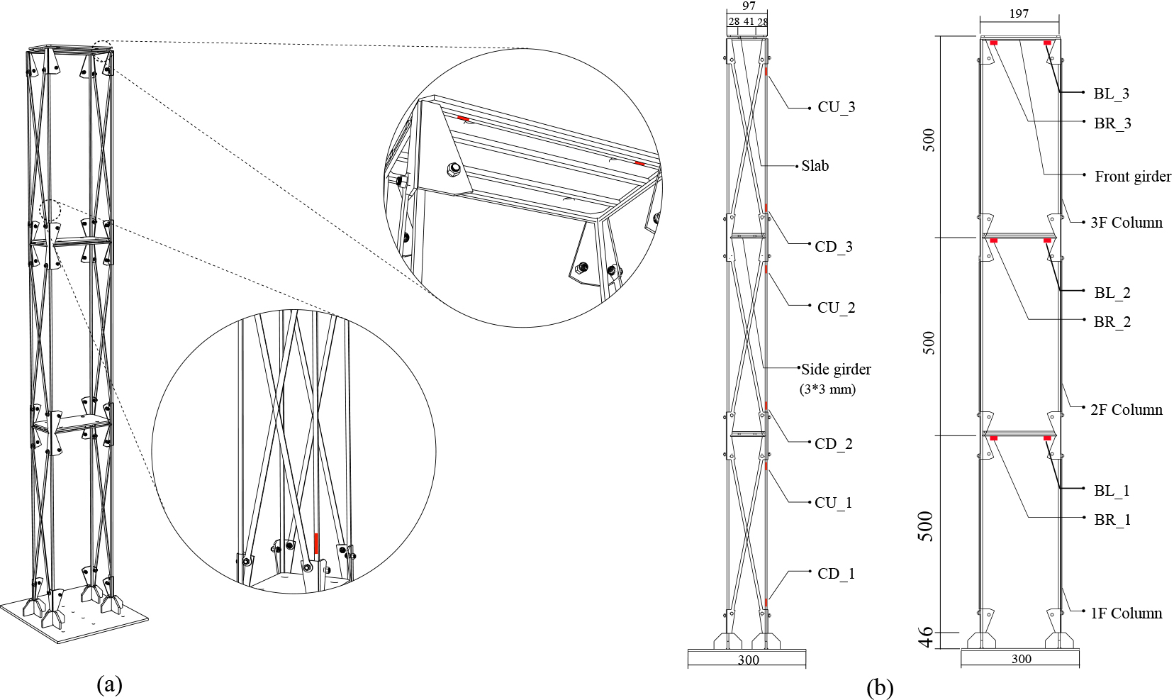
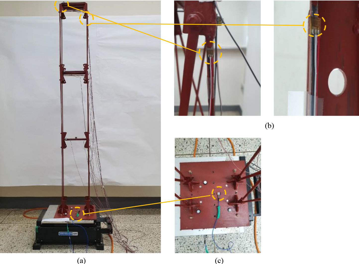
Figure 11.
Photo of experiment: (a) specimen on shaker; (b) strain sensor; and (c) accelerometer.
3.2.1Descriptions of specimen
In order to examine the practical applicability of the strain estimation technique proposed in this study, an experimental study using experimental models was carried out. The specimen used is a steel frame structure shown in Fig. 10a. The specimen consists of beams and columns comprising a total of three floors, with each floor measuring 0.5 m high. The length of the long side with no braces installed and the length of the short side with braces are shown in Fig. 10b. The specimen is installed on a shaking table, and the structural response to various seismic waves is measured. The experiment is performed with vibrations in one direction, which is the long side direction without braces. Braces were installed in the short side direction to restrain the torsion of the specimen. Through the shaking table test, the strain responses of the beam and column in the specimen were measured and used to validate the proposed technique. The locations of sensors installed in the beam and column for strain measurement are shown in Fig. 10b. Figure 11 shows photos of the specimen, strain sensor and accelerometer installed for ground acceleration measurement.
Figure 12.
Strain measurements of a column and beam on the 3rd floor subjected to a seismic wave.
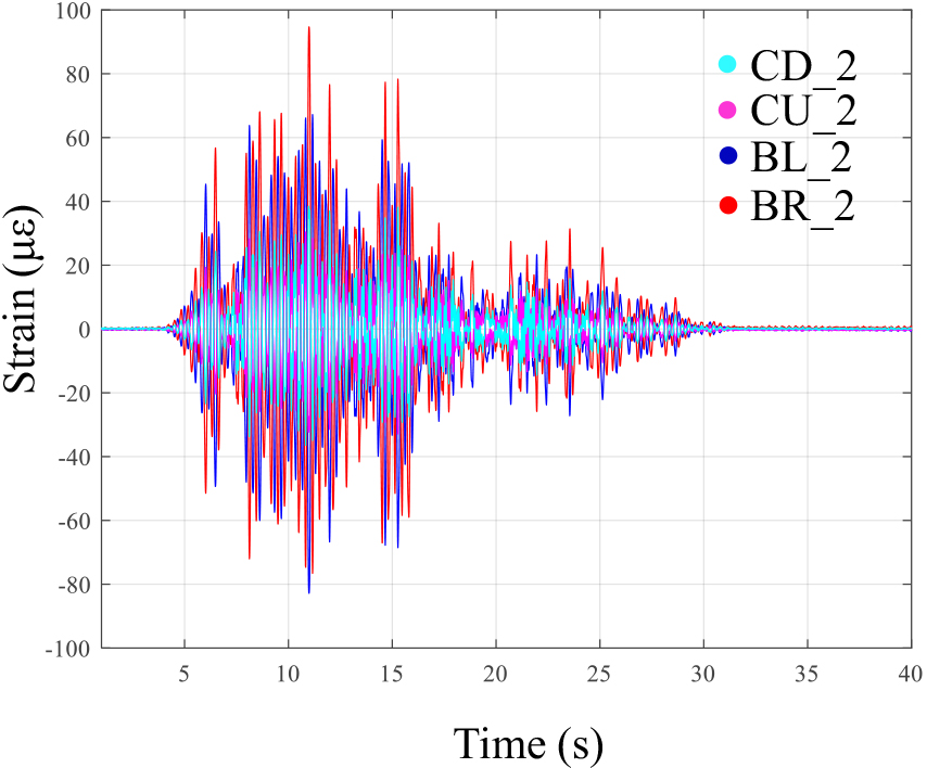
Strain measurement experiments were performed to verify the proposed technique. The shaking table test was conducted on a total of 20 seismic waves used in the simulation study. Information on the seismic waves can be found in the author’s research [47]. As an example, the structural strain response to a seismic wave measured in the beam and column in the third floor during the shaking table test is presented in Fig. 12.
Prior to examining the strain response prediction performance of the proposed technique, correlation analysis was performed to select the optimal CNN model for strain estimation. Pearson correlation analysis between beams and columns constituting the specimen was carried out, and the results are shown in Fig. 13. The strain responses measured from columns in each floor have high degrees of correlation with the strain responses measured from the adjacent beams as shown in Fig. 13. The strain measurement location used to build the optimal CNN model for strain estimation of a specific structural member is selected based on the results.
3.2.2Results of strain estimation
Figure 13.
Correlation coefficient of strain measurements from the experimental specimen.
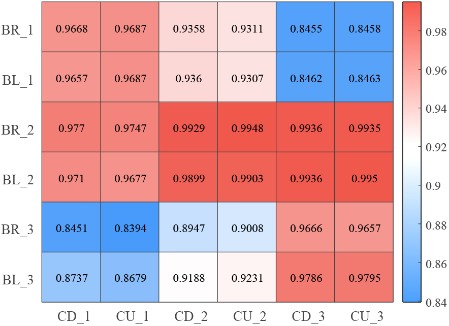
In the experimental study, the proposed technique using the measured strain response of the specimen was applied. The second-floor column (CU_2) in the specimen was selected as the target for strain estimation. The optimal CNN model selection based on correlation analysis was conducted to estimate the strain response of the second-floor beam. As shown in Fig. 13 the strain responses measured at the left and right ends of the second-floor beam (BR_2 and BL_2) with the highest degree of correlation with the strain response of the second-floor column were used to train the optimal CNN model The ground acceleration response was used in the input layer of the CNN model along with the strain response of the second-floor beam, while the strain response of the second-floor column was used in the output layer of the CNN model. The CNN architecture in this experimental study is identical to the one in the numerical study. Among the 20 earthquakes used in the shaking table test, 18 earthquakes were used to train the optimal CNN model The measured responses to two earthquakes, which were the 19th and 20th earthquakes in the literature [47]) and were not used in the CNN training, were used as test datasets to validate the trained CNN model.
Figure 14.
Optimal CNN training results for predicting strain of the 2nd floor column using strains of the 2nd floor beams: (a) convergence curve and (b) strain estimation results.
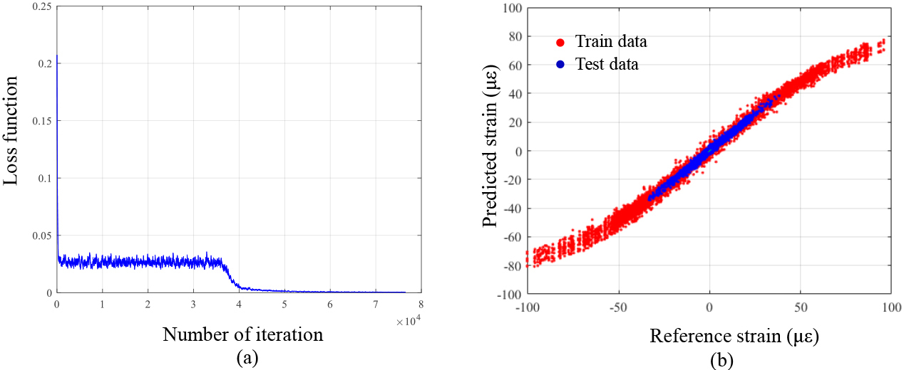
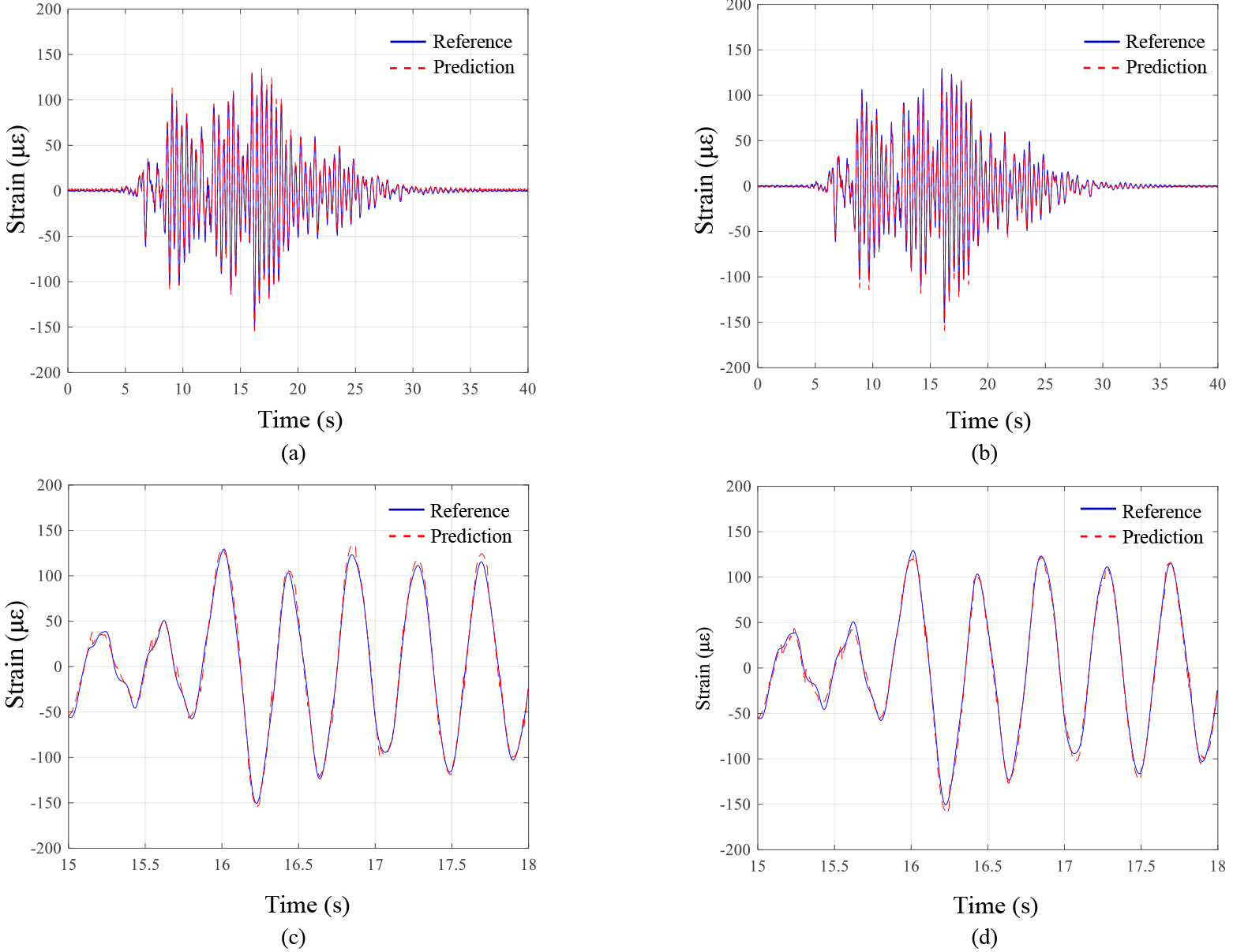
Figure 15.
Prediction of time series of strain of the 2nd floor column using the strain of the 2nd floor beam: (a) sub-jected to the 19th seismic wave; (b) subjected to the 20th seismic wave; (c) enlarged plot of Fig. 15a; and (d) enlarged plot of Fig. 15b.
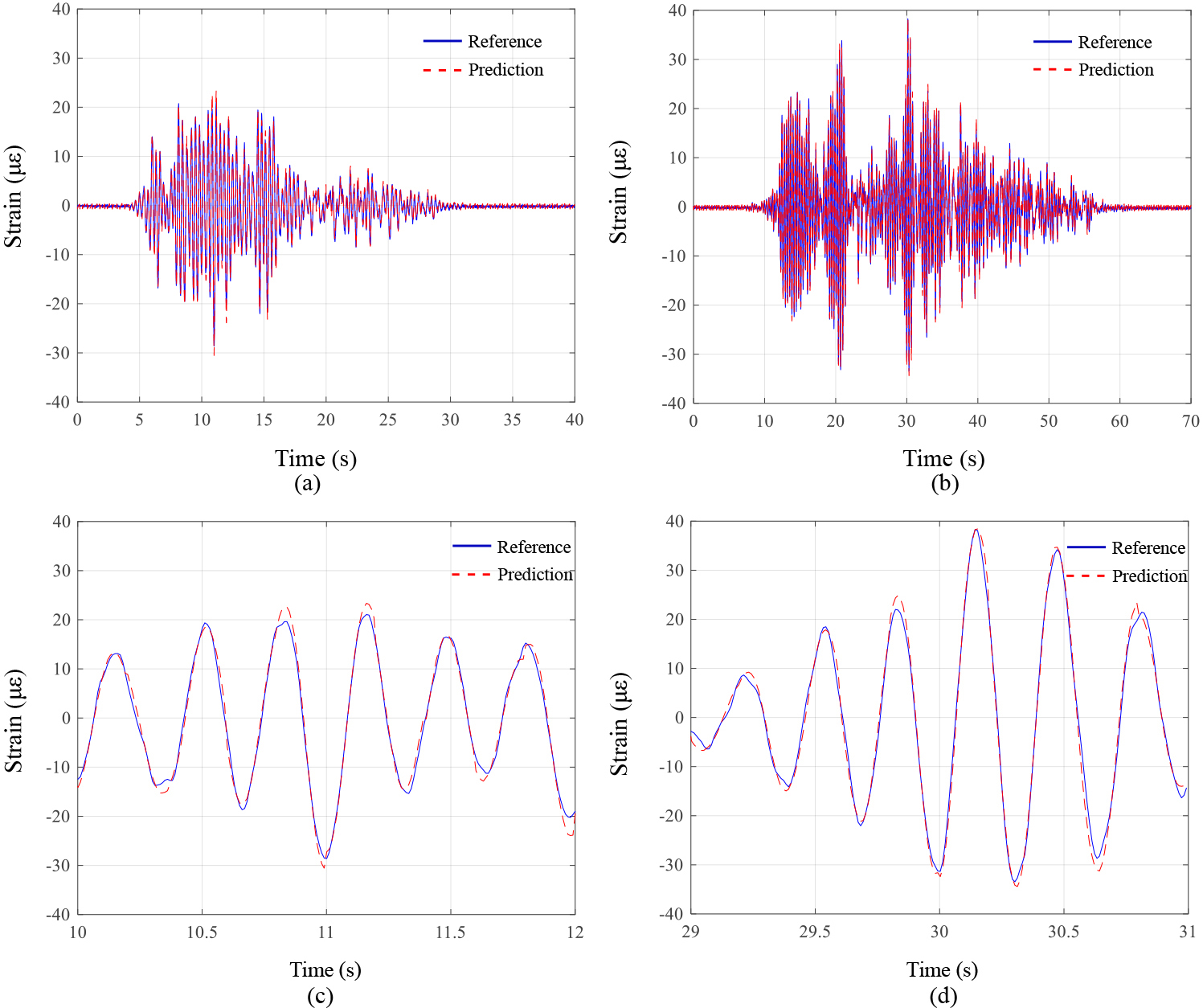
Figure 16.
Comparison of strain prediction according to the variation in correlation coefficient.
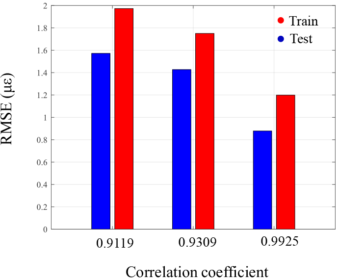
Figure 17.
Comparison of strain prediction according to the variation in the CNN input size: (a) RMSE and (b) computational cost.
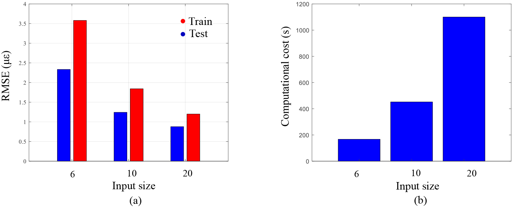
Figure 18.
Optimal CNN training results subjected to the 16th and 17th seismic waves (case 2): (a) convergence curve; (b) strain estimation results.
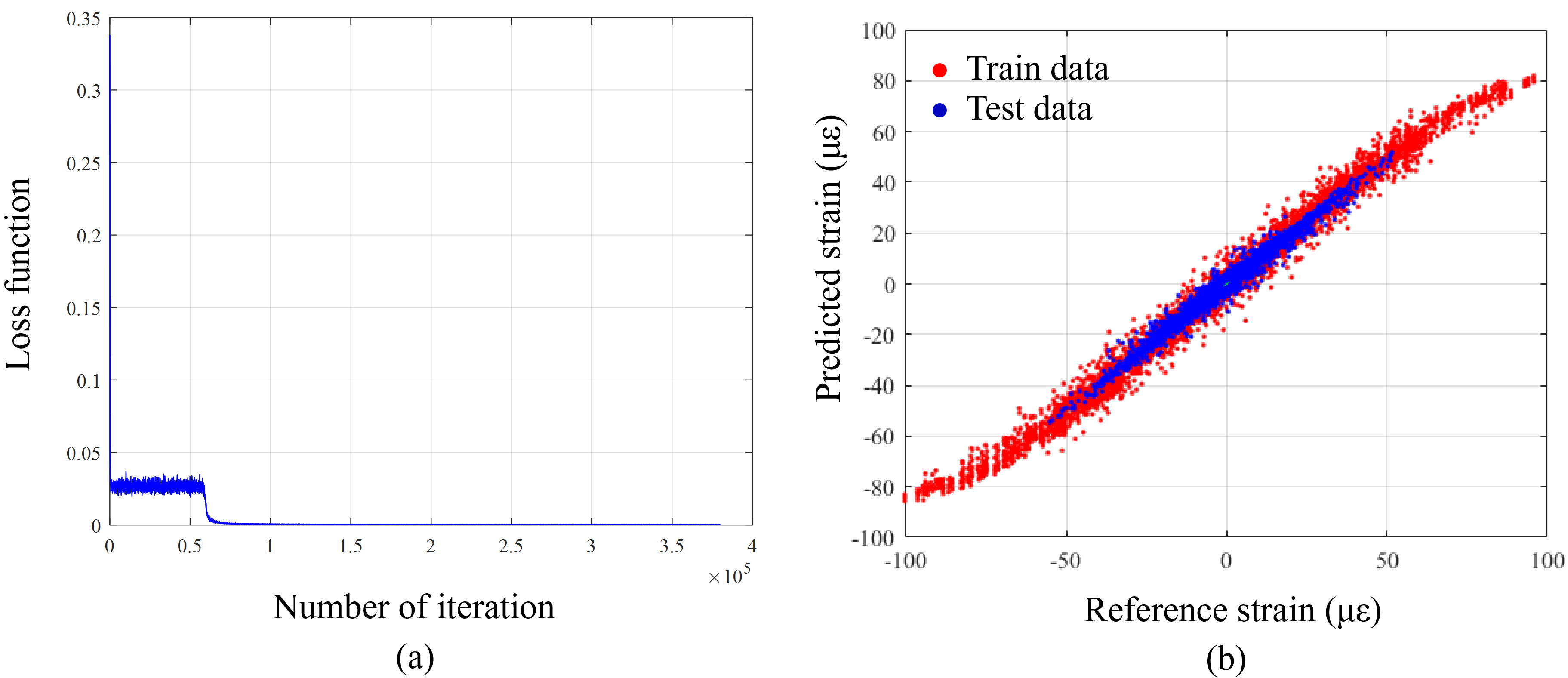
Figure 19.
Prediction of time series of strain of the 2nd floor column: (a) subjected to the 16th seismic wave; (b) subjected to the 17th seismic wave; (c) enlarged plot of Fig. 19(a); and (d) enlarged plot of Fig. 19(b).
The optimal CNN training results are shown in Fig. 14. Figure 14a shows the convergence curve of the loss function during CNN training. It was confirmed that the loss function decreased rapidly at the beginning of training and exhibited a rapid decrease once more at the middle of training, showing stable convergence. Figure 14b shows the strain estimation results for the training and test datasets of the trained optimal CNN model RMSE values were 1.1987 and 0.8785, respectively, for the training and test datasets, indicating that a CNN model with high estimation performance has been trained.
Figure 15 shows the results of the study that examined the prediction performance of the optimal CNN model in terms of the time history of the strain response. The estimation results for the time history of the strain of the second-floor column subjected to the 19th and 20th earthquakes, which were not used for CNN training, are given in Fig. 15a and 15b. The reference value and estimated values by the optimal CNN model showed high degrees of agreement. The RMSEs between the estimated and reference values were 0.7559 and 0.9471 for the 19th and the 20th earthquakes, respectively In order to examine the estimation results for a range with a relatively high amplitude among the time history of strain responses, an enlarged view of the section was examined. Figure 15c and 15d show enlarged views of the ranges with high amplitude of the response values for the 19th and 20th earthquakes. The optimal CNN model was capable of estimating the response accurately even in the range where a large deformation took place.
The proposed technique is essentially based on the optimal CNN selection based on correlation analysis. To confirm the validity of the present research technique for selecting the optimal CNN model through correlation coefficient analysis, a CNN model using responses with low degrees of correlation with the structural responses of the target structural member was trained, and its prediction performance was confirmed. The CNN model was trained using the strain response at the left and right ends of the third-floor beam (BR_3 and BL_3), which had a low degree of correlation with the response of the second-floor column (CU_2). Similar to the verification of the response prediction performance of the optimal CNN shown above, the strain prediction performance of the CNN model trained using the third-floor beam response was examined. Results showed RMSEs for the training dataset and the test dataset were 1.5720 and 1.9728, respectively, which were less accurate when compared to the optimal CNN model. This study confirmed the response prediction results of CNNs according to the correlation between the second-floor column strain data and all the beam strain data. Figure 16 shows the arithmetic mean of the correlation coefficient values between the responses at the left and right ends of the beam for each floor and the column on the second floor and RMSEs of corresponding CNNs. It was confirmed that higher degree of correlation results in greater strain estimation performance of the CNN This in turn verified the validity of the Pearson correlation analysis process for the optimal CNN model selection included in the proposed technique.
This study also examined the structural response prediction performance according to the variation in the CNN input size. The size at the CNN input layer of the measured data used in the above research results was 20
The above research results were limited to a dataset partitioning, which means 18 earthquakes including from 1st to 18th earthquakes in the literature [47] were selected for the training dataset while the remaining 2 earthquakes such as 19th and 20th earthquakes in the literature [47] were selected for the test dataset. This data constitution refers to case 1. In this part, the estimation performance of the presented method subjected to another data partitioning was investigated. In this case, 16th and 17th earthquakes in the literature [47] were selected to test datasets. Remaining earthquakes such as from the 1st to 15th earthquakes and from 18th to 20th earthquakes were selected for the training datasets. Another data constitution refers to case 2. The strain responses of the 2nd floor column (CU_2) and 2nd floor beams (BR_2 and BL_2), which have the highest correlation coefficients and used in the above examination (case 1) were used to train the optimal CNN. All conditions in this investigation were identical to the above case (case 1). The CNN was trained and the training results are shown in Fig. 18.
Figure 18a shows the convergence curve of the loss function. Figure 18b shows the estimation results for training and test datasets. RMSE values were 1.1269 and 1.1954, respectively, for the training and test datasets. Although the optimal CNN in this investigation estimated strain responses with relative accuracy, the RMSE values were slightly higher than those of the above estimation case (1.1987 and 0.8785, respectively, for the training and test datasets). It was regarded that the higher error stems from the response range for test datasets in case 2 was wider than the above case 1, which means more responses for test datasets in case 2 had nonlinearity than case 1. The estimation performance of the optimal CNN was also examined in terms of the time history of strain responses. Figure 19 showed the prediction results. It was confirmed that the optimal CNN efficiently predicted the time series responses subjected to the 16th and 17th earthquakes.
4.Conclusions
A correlation analysis-based strain estimation technique for building structures was presented. The relationship between the strain responses of several structural members in the structure was determined using a CNN model for strain estimation. The optimal CNN model for strain response estimation was selected based on the correlational analysis between responses measured from the structural members. The proposed technique was applied to the analytical study for strain estimation of the ASCE benchmark model Applicability of the proposed technique was also examined through a shaking table test on a 3-story steel frame specimen. Through analytical and experimental studies, the strain estimation performance of the proposed technique was validated. The RMSEs for test datasets in the experimental study were 0.8785 and 1.1954 for case 1 and case 2, respectively. The RMSE values correspond to 2.30% and 2.17% of the maximum strain responses of the target structural member for test datasets, demonstrating the precision of the presented method. The adequacy of the data types in the input map configuration of CNN in the technique, such as the utilization of ground acceleration responses and the number of response locations, was likewise verified. Furthermore, the validity of the correlation analysis method between the responses of structural members for the optimal CNN section was confirmed. The response estimation performance of the proposed technique according to the variation of the CNN input size was also examined.
As confirmed in the prediction results for case 2, the error for the test dataset was higher than case 1. The test dataset in case 2 had a wider strain response range than case 1, which indicates test datasets in case 2 had more nonlinearity than those in case 1. From this comparison, it was regarded that the presented method can be limited to the datasets including large nonlinearity. As the nonlinear data particularly including residual deformation can be extracted in case of occurring damage in the structure, the presented method can also be limited to the datasets from damaged structures. In future studies, some prediction methods for the datasets including nonlinearity will be focused based on the data driven approach with frequency domain data as well as time domain data [48]. In addition, the CNN architecture employed in the study was derived by modifying the author’s previous works [47] that dealt with time series of structural responses. Even if the used architecture in this study showed relatively accurate performance, there is still room for progress by investigating some methods to find the optimal architectures, which will be another research focus for the authors in the future. Furthermore, to improve the prediction capacity of the present method, the applicability of more powerful and sophisticated supervised machine learnings [49, 50, 51] will be investigated in the future works.
Acknowledgments
This work was supported by a National Research Foundation of Korea (NRF) grant funded by the Korean government (Ministry of Science, ICT & Future Planning, MSIP) (NRF-2018R1A5A1025137 and NRF-2022R1C1C1009871).
References
[1] | Amezquita-Sanchez JP, Adeli H. Synchrosqueezed wavelet transform-fractality model for locating, detecting, and quantifying damage in smart highrise building structures. Smart Mater. Struct. (2015) ; 24: : 065034. |
[2] | Pavlou D. A deterministic algorithm for nonlinear, fatigue-based structural health monitoring. Comput. Civ. Infrastruct. Eng. (2022) ; 37: (7): 809-31. |
[3] | Hormozabad SJ, Gutierrez Soto M, Adeli H. Integrating structural control, health monitoring, and energy harvesting for smart cities. Expert Syst. (2021) ; 38: : e12845. |
[4] | Yang HTY, Shan J, Randall CJ, Hansma PK, Shi W. Integration of health monitoring and control of building structures during earthquakes J. Eng. Mech. (2014) ; 140: : 04014013. |
[5] | Xu J, Liu H, Han Q. Blockchain technology and smart contract for civil structural health monitoring system. Comput. Civ. Infrastruct. Eng. (2021) ; 36: (10): 1288-1305. |
[6] | Jhao J, Hu F, Xu Y, Zuo W, Zhong J, Li H. Structure-PoseNet for identification of dense dynamic displacement and 3D poses of structures using a monocular camera. Comput. Civ. Infrastruct. Eng. (2022) ; 37: (6): 704-25. |
[7] | Nasimi R, Moreu F. A methodology for measuring the total displacements of structures using a laser-camera system. Comput. Civ. Infrastruct. Eng. (2021) ; 36: (4): 421-37. |
[8] | Ngeljaratan L, Moustafa MA, Pekcan G. A compressive sensing method for processing and improving vision-based target-tracking signals for structural health monitoring. Comput. Civ. Infrastruct. Eng. (2021) ; 36: (9): 1203-23. |
[9] | Sun J, Peng B, Wang CC, Chen K, Zhong B, Wu J. Building displacement measurement and analysis based on UAV images. Autom. Constr. (2022) ; 140: : 104367. |
[10] | Rafiei MH, A novel machine learning-based algorithm to detect damage in high-rise building structure Struct. Design Tall Spec. (2017) ; 26: : e1400. |
[11] | Li Z, Park HS, Adeli H. New method for modal identification and health monitoring of superhighrise building structures using discretized synchrosqueezed wavelet and hilbert transforms, Struct. Design Tall Spec. (2017) ; 26: (3): e1312. |
[12] | Amezquita-Sanchez JP, Park HS, Adeli H. A novel methodology for modal parameters identification of large smart structures using MUSIC, empirical wavelet transform, and Hilbert transform. Eng. Str. (2017) ; 147: : 148-59. |
[13] | Perez-Ramirez CA, Amezquita-Sanchez JP, Adeli H, Valtierra-Rodriguez M, Camarena-Martinez D, Rene Romero-Troncoso RJ. New methodology for modal parameters identification of smart civil sructures using ambient vibrations and synchrosqueezed wavelet. Eng. Appl. Artif. Intell. (2016) ; 24: : 1-16. |
[14] | Zhang Q, Zhang J. Internal force monitoring and estimation of a long-span ring beam using long-gauge strain sensing. Comput. Civ. Infrastruct. Eng. (2021) ; 36: (1): 109-24. |
[15] | Yan M, Tan X, Mahjoubi S, Bao Y. Strain transfer effect on measurements with distributed fiber optic sensors. Autom. Constr. (2022) ; 139: : 104262. |
[16] | Park HS, Jung SM, Lee HM, Kwon YH, Seo JH. Analytical models for assessment of the safety of multi-span steel beams based on average strains from long gage optic sensors. Sens. Actuator A Phys. (2007) ; 137: (1): 6-12. |
[17] | Hampshire TA, Adeli H. Monitoring the behavior of steel structures using distributed optical fiber sensors. J. Constr. Steel Res. (2000) ; 53: (3): 267-81. |
[18] | Lee HM, Choi SW, Jung D, Park HS. Analytical model for estimation of maximum normal stress in steel beam-columns based on wireless measurement of average strains from vibrating wire strain gages. Comput. Civ. Infrastruct. Eng. (2013) ; 28: (9): 707-17. |
[19] | Choi SW, Lee J, Oh BK, Park HS, Analytical models for estimation of the maximum strain of beam structures based on optical fiber Bragg grating sensors. J. Civ. Eng. Manag. (2016) ; 22: (1); 86-91. |
[20] | Lu W, Teng J, Li C, Cui Y. Reconstruction to sensor measurements based on a correlation model of monitoring data. Appl. Sci. (2017) ; 7: (3): 234. |
[21] | Amezquita-Sanchez JP, Valtierra-Rodriguez M, Adeli H. Wireless smart sensors for monitoring the health condition of civil infrastructure. Sci. Iran. (2018) ; 25: (6): 2913-25. |
[22] | Shajihan SAV, Hoang T, Mechitov K, Spencer BF. Wireless smart vision system for synchronized displacement monitoring of railroad bridges. Comput. Civ. Infrastruct. Eng. (2022) ; 37: (9): 1070-88. |
[23] | Avci O, Abdeljaber O, Kiranyaz S, Hussein M, Inman DJ. Wireless and real-time structural damage detection: A novel decentralized method for wireless sensor networks. J. Sound Vib. (2018) ; 424: : 158-72. |
[24] | Yu Y, Han F, Bao Y, Ou J. A study on data loss compensation of WiFi-based wireless sensor networks for structural health monitoring. IEEE Sens. J. (2016) ; 16: (10): 3811-18. |
[25] | Chen Z, Li H, Bao Y. Analyzing and modeling inter-sensor relationships for strain monitoring data and missing data imputation: a copula and functional data-analytic approach. Struct. Health Monit. (2019) ; 18: (4): 1168-88. |
[26] | Zhang Z, Luo Y. Restoring method for missing data of spatial structural stress monitoring based on correlation. Mech. Syst. Signal Process. (2017) ; 91: : 266-77. |
[27] | Skafte A, Kristoffersen J, Vestermark J, Tygesen UT, Brincker R. Experimental study of strain prediction on wave induced structures using modal decomposition and quasi static Ritz vectors. Eng. Struct. (2017) ; 136: : 261-76. |
[28] | Bharadwaj K, Sheidaei A, Afshar A, Baqersad J, Full-field strain prediction using mode shapes measured with digital image correlation. Measurement. (2019) ; 139: : 326-33. |
[29] | Wang YW, Ni YQ. Bayesian dynamic forecasting of structural strain response using structural health monitoring data. Struct. Control and Health Monit. (2020) ; 27: (8): e2575. |
[30] | Rafiei MH, Adeli H. A novel machine learning model for estimation of sale prices of real estate units. J. Constr. Eng. Manag. (2016) ; 142: (2): 04015066. |
[31] | Rafiei MH, Khushefati WH, Demirboga R, Adeli H. Supervised deep restricted boltzmann machine for estimation of concrete compressive strength. ACI Mater. J. (2017) ; 114: (2): 237-44. |
[32] | Adeli H. Neural networks in civil engineering: 1989–2000. FEMa: a finite element machine for fast learning. Comput. Civ. Infrastruct. Eng. (2001) ; 16: (2): 126-42. |
[33] | Nogay HS, Adeli H. Machine learning for the diagnosis of autism spectrum disorder using brain imaging. Reviews in the Neurosciences (2020) ; 31: (8): 825-41. |
[34] | Perez-Ramirez CA, Amezquita-Sanchez JP, Valtierra-Rodriguez M, Adeli H, Dominguez-Gonzalez A, Romero-Troncoso RJ, Osornio-Rios RA. Recurrent neural network model with Bayesian training and mutual information for response prediction of large buildings. (2019) ; 178: : 603-15. |
[35] | Oh BK, Kim KJ, Kim Y, Park HS, Adeli H. Evolutionary learning-based sustainable strain sensing model for structural health monitoring of high-rise buildings. Appl. Soft Comput. (2017) ; 58: : 576-85. |
[36] | Kromanis R, Kripakaran P. Support vector regression for anomaly detection from measurement histories. Adv. Eng. Inform. (2013) ; 27: : 486-95. |
[37] | Wang F, Song G, Mo YL. Shear loading detection of through-bolts in bridge structures using a percussion-based one-dimensional memory-augmented convolutional neural network. Comput. Civ. Infrastruct. Eng. (2021) ; 36: (3): 289-301. |
[38] | Xue Y, Jiang P, Neri F, Liang J. A multiobjective evolutionary approach based on graph-in-graph for neural architecture search of convolutional neural networks. Int. J. Neural Syst. (2021) ; 31: (9): 2150035. |
[39] | Peng P, Xie L, Wei H. A deep Fourier neural network for seizure prediction using convolutional neural network and ratios of spectral power. Int. J. Neural Syst. (2021) ; 31: (8): 2150022. |
[40] | Sarlo R. Toward a general unsupervised novelty detection framework in structural health monitoring, Comput. Civ. Infrastruct. Eng. (2022) ; 37: (9): 1128-45. |
[41] | Sajedi SM, Liang X. Deep Generative Bayesian Optimization for Sensor Placement in Structural Health Monitoring. Comput. Civ. Infrastruct. Eng. (2022) ; 37: (9): 1109-27. |
[42] | Gulgec NS, Takac M, Pakzad SN. Structural sensing with deep learning: Strain estimation from acceleration data for fatigue assessment. Comput. Civ. Infrastruct. Eng. (2020) ; 35: (12): 1349-64. |
[43] | Chen C, Tang L, Lu Y, Wang Y, Liu Z, Liu Y, Zhou L, Jiang Z, Yang B. Reconstruction of long-term strain data for structural health monitoring with a hybrid deep-learning and autoregressive model considering thermal effects. Eng. Struct. (2023) ; 285: : 116063. |
[44] | Johnson EA, Lam HF, Katafygiotis LS, Beck JL. Phase I IASC-ASCE structural health monitoring benchmark problem using simulated data. J. Eng. Mech. (2004) ; 130: (1): 3-15. |
[45] | Abdeljaber O, Avci O, Kiranyaz MS, Boashash B, Sodano H, Inman DJ. 1-D CNNS for structural damage detection: Verification on a structural health monitoring benchmark data. Neurocomputing. (2018) ; 275: : 1308-17. |
[46] | Pacific Earthquake Engineering Research Center (PEER), OpenSees: Open System for Earthquake Engineering Simulation, University of California, Berkeley, CA. |
[47] | Oh BK, Park Y, Park HS. Seismic response prediction method for building structures using convolutional neural network. Struct. Control Health Monitor. (2020) ; 27: (5): e2519. |
[48] | Amezquita-Sanchez JP, Adeli H, A new MUSIC-Empirical wavelet transform methodology for time-frequency analysis of noisy nonlinear and non-stationary signals. Digit. Signal Process. (2015) ; 45: : 55-68. |
[49] | Rafiei MH, Adeli H. A new neural dynamic classification algorithm, IEEE Transactions on Neural Networks and Learning Systems. IEEE T. Neur. Net. Lear. (2017) ; 28: (12): 3074-83. |
[50] | Pereira DR, Piteri MA, Souza AN, Papa J, Adeli H. FEMa: A finite element machine for fast learning, Neural. Comput. Appl. (2020) ; 32: (10): 6393-04. |
[51] | Alam KMR, Siddique N, Adeli H. A dynamic ensemble learning algorithm for neural networks, Neural. Comput. Appl. (2020) ; 32: (10): 8675-90. |

