


The European Study Group with Industry that motivated the work in this manuscript is one of many such that Graeme Hocking regularly attends, in Limerick and around the world, often as Moderator, and always as an enthusiastic expert. We are pleased to be able to contribute this research paper to a special edition honouring Professor Hocking’s significant global contributions to industrial mathematics over many years.
1 Introduction
The use of low-powered microwaves to automatically detect moisture content of powder or bulk solids in real time on a conveyor belt is key for the pricing and control of a number of industrial processes, including ore, coal, bauxite, grains, seeds, pelleted biomass and pharmaceuticals. However, the technology in use does not always reflect a good understanding of the effects of varying setups and conditions on analyser reliability.
We present an example of microwave use in the bauxite industry, and show how it benefits from the improved understanding that applied mathematics provides. Our example comes from a challenge that was brought to the 128th European Study Group with Industry (ESGI) in 2017 at the University of Limerick in Ireland. Bauxite electromagnetic measurements taken by an automatic microwave analyser during offload from a ship to an alumina factory were provided to the Study Group, and have provided the guiding impetus for our modelling efforts. The measurements show that while phase shift data from the analyser provide a useful indication of moisture content, signal attenuation data do not look helpful [Reference McGuinness, Bohun, Cregan, Lee, Dewynne, O’Keeffe, Vo, McKibbin, Wake and Saeki12]. The algorithms used in the analyser are based on linear regression models using both signal strength and phase shift. However, the signal attenuation recorded by the analyser and reported by McGuinness et al. [Reference McGuinness, Bohun, Cregan, Lee, Dewynne, O’Keeffe, Vo, McKibbin, Wake and Saeki12] is strongly nonlinear when plotted against bauxite height (depth). It has been speculated [Reference McGuinness, Bohun, Cregan, Lee, Dewynne, O’Keeffe, Vo, McKibbin, Wake and Saeki12] that internal reflections and wave interference might account for the highly oscillatory behaviour seen in attenuation data from the analyser.
This effect of reflections of microwaves is avoided in applications where measurements are taken across material flowing down a circular cross-section, so that the average thickness of the material is constant and there is a curved interface between material and air. Then thickness can be ignored, while density variations have a significant effect on measurements and moisture content inference [Reference Nelson and Trabelsi15].
We present a new mathematical model of microwave travel through a layer of bauxite with air gaps above and below. The meaning of the word model is broad, and in [Reference Viana21], for example, it is applied to the use of a simple linear regression model to infer bauxite moisture content. Moisture content is taken to be proportional to phase shift divided by total mass, and to attenuation divided by total mass. Density and height (depth) of bauxite both affect total mass, which may also be measured directly on a conveyor belt. However, Viana [Reference Viana21] found that using belt tonnage scales to measure mass led to unreliable and inaccurate analyser values for moisture content, when using the analyser in an alumina plant in Brazil. Instead, they obtained more reliable results if they used measurements of material height instead of mass, thereby assuming constant material porosity.
Viana [Reference Viana21] uses the same regression formula as the one used in the microwave analyser that provided our data from the ESGI, in which the moisture content M (mass of water per unit mass of moist bauxite mixture) is given by
 $$ \begin{align} M = c_0 + c_1 \frac{\Delta \phi}{h} + c_2 \frac{L}{h} , \end{align} $$
where the constants
 $c_0$
,
$c_0$
,
 $c_1$
and
$c_1$
and
 $c_2$
are fitted during calibration to the moisture content of laboratory samples,
$c_2$
are fitted during calibration to the moisture content of laboratory samples,
 $\Delta \phi $
is the phase shift (radians) in the complex valued electric field
$\Delta \phi $
is the phase shift (radians) in the complex valued electric field
 $E(h)$
signal at the receiving antenna when bauxite height is h, and L is the signal attenuation, given in dB by
$E(h)$
signal at the receiving antenna when bauxite height is h, and L is the signal attenuation, given in dB by
 $$ \begin{align} L = -20 \log _{10} \bigg | \frac{E(h)}{E(0)} \bigg |. \end{align} $$
This form for attenuation is also referred to as the electromagnetic shielding efficiency [Reference Vojtech, Neruda and Hajek22] of the bauxite material. The phase shift is the difference in radians between the phase or argument of the complex number
 $E(h)$
and the phase or argument of
$E(h)$
and the phase or argument of
 $E(0)$
(recorded when the conveyor belt is empty).
$E(0)$
(recorded when the conveyor belt is empty).
Such a simple model is noted to require careful and frequent calibration of the analyser [Reference Viana21], and careful treatment of the lab samples used to calibrate. Special care is needed to ensure that sample times match analyser times [Reference McGuinness, Bohun, Cregan, Lee, Dewynne, O’Keeffe, Vo, McKibbin, Wake and Saeki12].
Rearranging the regression formula (1.1) and assuming constant moisture content then requires that phase shift divided by h is constant, and that attenuation divided by h is constant. That is, if moisture content does not change much, then phase shift and attenuation must both be proportional to or linear in h. There is some support in Figure 1 for measured phase shifts being linear in bauxite height, but it is clear that attenuation is highly oscillatory and a linear approximation is going to perform poorly [Reference McGuinness, Bohun, Cregan, Lee, Dewynne, O’Keeffe, Vo, McKibbin, Wake and Saeki12].

Figure 1 Microwave analyser data recorded while unloading bauxite from the ship Maia. The phase shift
 $\Delta \phi $
(radians) and signal strength (
$\Delta \phi $
(radians) and signal strength (
 $-L$
, the negative of attenuation; in arbitrary units for these data) are plotted against bauxite height.
$-L$
, the negative of attenuation; in arbitrary units for these data) are plotted against bauxite height.
1.1 Maxwell’s equations
The regression formula (1.1) used by the microwave analyser may be justified by considering a more sophisticated kind of model for microwave propagation in bauxite. Maxwell’s equations for electromagnetic propagation in a stationary linear isotropic conducting dielectric material may be written in the form [Reference Lorrain, Corson and Lorrain10]
 $$ \begin{align} \nabla \cdot \mathbf{E} &= \rho_f/\epsilon , \end{align} $$
 $$ \begin{align}\nabla \cdot \mathbf{B} &= 0 , \end{align} $$
 $$ \begin{align}\nabla \times \mathbf{E} &= - \frac{\partial \mathbf{B}}{\partial t}, \end{align} $$
 $$ \begin{align} \nabla \times \mathbf{H} &= \epsilon \frac{\partial \mathbf{E}}{\partial t} + \mathbf{J}_f + \frac{\partial \mathbf{P}}{\partial t}, \end{align} $$
where
 $\mathbf {E}$
is the electric field intensity,
$\mathbf {E}$
is the electric field intensity,
 $\mathbf {P}$
is the polarization field of the dielectric,
$\mathbf {P}$
is the polarization field of the dielectric,
 $\mathbf {H}$
the magnetic field intensity,
$\mathbf {H}$
the magnetic field intensity,
 $\mathbf {B} = \mu _0(\mathbf {H}+\mathbf {M}) = \mu \mathbf {H}$
is the magnetic induction,
$\mathbf {B} = \mu _0(\mathbf {H}+\mathbf {M}) = \mu \mathbf {H}$
is the magnetic induction,
 $\mathbf {J}_f$
is the free current density,
$\mathbf {J}_f$
is the free current density,
 $\mathbf {M}$
is the magnetization and
$\mathbf {M}$
is the magnetization and
 $\rho _f$
the free charge density. The permittivity of free space (vacuum or air) is
$\rho _f$
the free charge density. The permittivity of free space (vacuum or air) is
 $\epsilon _0 = 8.85 \times 10^{-12}$
F/m and the permeability of free space is
$\epsilon _0 = 8.85 \times 10^{-12}$
F/m and the permeability of free space is
 $\mu _0 = 4\pi \times 10^{-7}$
H/m which corresponds to the propagation speed (of light)
$\mu _0 = 4\pi \times 10^{-7}$
H/m which corresponds to the propagation speed (of light)
 $c = (\epsilon _0\mu _0)^{-1/2} \approx 3\times 10^8$
m/s.
$c = (\epsilon _0\mu _0)^{-1/2} \approx 3\times 10^8$
m/s.
Boundary conditions at the interfaces between bauxite and air invoke continuity of normal and tangential electric and magnetic fields
 $$ \begin{align*} [\epsilon \mathbf{E} \cdot \mathbf{n} ] _- ^+ = 0 , \; \; [\epsilon \mathbf{H} \cdot \mathbf{n} ] _- ^+ = 0 , \; \; [ \mathbf{E} \times \mathbf{n} ] _- ^+ = 0 , \; \; [ \mathbf{H} \times \mathbf{n} ] _- ^+ = 0 ,\end{align*} $$
where
 $\mathbf {n} $
is the unit normal to the interface, and the notation
$\mathbf {n} $
is the unit normal to the interface, and the notation
 $ [f]_-^+ = f^+ - f_-$
means the change in f across the interface.
$ [f]_-^+ = f^+ - f_-$
means the change in f across the interface.
We treat the bauxite as a conducting dielectric porous medium, a material which is a mixture of solid, liquid and air. This mixture is considered to have an effective scalar conductivity
 $\sigma _b$
and an effective scalar permittivity
$\sigma _b$
and an effective scalar permittivity
 $\epsilon _b$
that vary with moisture content, bauxite type and air content.
$\epsilon _b$
that vary with moisture content, bauxite type and air content.
Polarization is taken to be in the same direction as
 $\mathbf {E}$
and proportional to it, so that
$\mathbf {E}$
and proportional to it, so that
 $\mathbf {P}=\epsilon _0\chi _e\mathbf {E}$
. The permittivity of the bauxite is written as
$\mathbf {P}=\epsilon _0\chi _e\mathbf {E}$
. The permittivity of the bauxite is written as
 $\epsilon _b =\epsilon _r \epsilon _0 = \epsilon _0 (1 + \chi _e) $
and the permeability of the bauxite is
$\epsilon _b =\epsilon _r \epsilon _0 = \epsilon _0 (1 + \chi _e) $
and the permeability of the bauxite is
 $\mu _b = \mu _r \mu _0 = \mu _0 (1+ \chi _m)$
. Note that
$\mu _b = \mu _r \mu _0 = \mu _0 (1+ \chi _m)$
. Note that
 $\mathbf {J}_f = \sigma \mathbf {E}$
.
$\mathbf {J}_f = \sigma \mathbf {E}$
.
Bauxite is usually considered to be nonmagnetic. However, it may contain maghemite, so that magnetization
 $\mathbf {M} = \chi _m \mathbf {H}$
may not be zero [Reference Kondrat’ev, Rostovtsev and Baksheeva7, Reference Mullins13, Reference Taylor, Eggleton, Foster, Tilley, Le Gleuher and Morgan17]. In soil science, a mass susceptibility or specific magnetic susceptibility is often calculated, which equals
$\mathbf {M} = \chi _m \mathbf {H}$
may not be zero [Reference Kondrat’ev, Rostovtsev and Baksheeva7, Reference Mullins13, Reference Taylor, Eggleton, Foster, Tilley, Le Gleuher and Morgan17]. In soil science, a mass susceptibility or specific magnetic susceptibility is often calculated, which equals
 $\chi _m/\rho $
, where
$\chi _m/\rho $
, where
 $\rho $
is the bulk density of the soil. This mass susceptibility needs to be multiplied by bulk density (typically approximately 1200 kg/m
$\rho $
is the bulk density of the soil. This mass susceptibility needs to be multiplied by bulk density (typically approximately 1200 kg/m
 $^3$
for mined bauxite) to obtain
$^3$
for mined bauxite) to obtain
 $\chi _m$
.
$\chi _m$
.
Bauxites with high iron content [Reference Kondrat’ev, Rostovtsev and Baksheeva7] have measured values
 $\chi _m \approx 3\times 10^{-4}$
. Maghemite has mass susceptibility around
$\chi _m \approx 3\times 10^{-4}$
. Maghemite has mass susceptibility around
 $9\times 10^{-4}$
m
$9\times 10^{-4}$
m
 $^3$
/kg [Reference Mullins13], so that its bulk magnetic susceptibility is
$^3$
/kg [Reference Mullins13], so that its bulk magnetic susceptibility is
 $\chi _m \approx 1$
. Weipa pisolith bauxite from Australia may contain up to 15% maghemite by mass [Reference Taylor, Eggleton, Foster, Tilley, Le Gleuher and Morgan17] suggesting
$\chi _m \approx 1$
. Weipa pisolith bauxite from Australia may contain up to 15% maghemite by mass [Reference Taylor, Eggleton, Foster, Tilley, Le Gleuher and Morgan17] suggesting
 $\chi _m \approx 0.15 n \approx 0.06$
for this bauxite if porosity
$\chi _m \approx 0.15 n \approx 0.06$
for this bauxite if porosity
 $n = 0.4$
.
$n = 0.4$
.
Hence,
 $\mu _r = 1 + \chi _m$
is likely to be close to one for bauxite, and we will use
$\mu _r = 1 + \chi _m$
is likely to be close to one for bauxite, and we will use
 $\mu _b = \mu _0$
. Magnetization is also taken to be zero in the region representing the receiving antenna in the four-layer model, so that magnetic susceptibilities in air and in the antenna are set to
$\mu _b = \mu _0$
. Magnetization is also taken to be zero in the region representing the receiving antenna in the four-layer model, so that magnetic susceptibilities in air and in the antenna are set to
 $\mu = \mu _0$
in the following.
$\mu = \mu _0$
in the following.
Our data are obtained at the operating frequency
 $f= 0.9$
GHz. At this frequency, water has
$f= 0.9$
GHz. At this frequency, water has
 $\epsilon _r \approx 80$
and
$\epsilon _r \approx 80$
and
 $\sigma \approx $
0.5–50 mS/m depending on how potable it is. Seawater has
$\sigma \approx $
0.5–50 mS/m depending on how potable it is. Seawater has
 $\epsilon _r \approx 80$
and
$\epsilon _r \approx 80$
and
 $\sigma \approx $
5000 mS/m. Properties for damp soil provide some guidance as to anticipated values for bauxite. Measured permittivity results reviewed in [Reference Dobson and Ulaby5] give for dryness near 0.02 (by volume, dry basis),
$\sigma \approx $
5000 mS/m. Properties for damp soil provide some guidance as to anticipated values for bauxite. Measured permittivity results reviewed in [Reference Dobson and Ulaby5] give for dryness near 0.02 (by volume, dry basis),
 $\epsilon _r \approx $
3 and
$\epsilon _r \approx $
3 and
 $\sigma \approx $
2 mS/m for nearly dry silts, while for dryness near 0.4 (by volume, dry basis),
$\sigma \approx $
2 mS/m for nearly dry silts, while for dryness near 0.4 (by volume, dry basis),
 $\epsilon _r \approx $
24 and
$\epsilon _r \approx $
24 and
 $\sigma \approx $
40 mS/m for very wet silts.
$\sigma \approx $
40 mS/m for very wet silts.
1.2 Differential equations
Taking the curl of (1.3c) and using
 $$ \begin{align*}\mathbf{\nabla \times \nabla \times E} = - \mathbf{\nabla ^2 E} + \mathbf{\nabla (\nabla \cdot E)} \end{align*} $$
gives
 $$ \begin{align*} \mathbf{\nabla ^2 E} - \mathbf{\nabla (\nabla \cdot E)} = \frac{\partial}{\partial t} \bigg ( \mu \epsilon \frac{\partial \mathbf{E}}{\partial t} + \mu \mathbf{J}_f + \mu \frac{\partial \mathbf{P}}{\partial t} \bigg ), \end{align*} $$
and in the absence of free charges and using (1.3a), this becomes a wave equation for the electric field, which for constant material properties is [Reference Lorrain, Corson and Lorrain10, Section 27.8]
 $$ \begin{align} \mathbf{\nabla ^2 E} - \mu \epsilon \frac{\partial^2 \mathbf{E}}{\partial t^2} - \mu \sigma \frac{\partial \mathbf{E}}{\partial t} = 0 \;. \end{align} $$
The same equation can be derived for the magnetic field strength
 $\mathbf {H}$
, with
$\mathbf {H}$
, with
 $\mathbf {H}$
replacing
$\mathbf {H}$
replacing
 $\mathbf {E}$
.
$\mathbf {E}$
.
1.3 Simple model
A simple model that motivates the regression formula used in the microwave analyser considers transmission of microwaves that travel through a thickness h of bauxite at a single frequency
 $\omega = 2 \pi f$
before detection at the receiving antenna. Without loss of generality, we consider a polarized signal with fixed directions in which field strengths vary. Choosing origin at the base of the bauxite and axes aligned appropriately, we have solutions
$\omega = 2 \pi f$
before detection at the receiving antenna. Without loss of generality, we consider a polarized signal with fixed directions in which field strengths vary. Choosing origin at the base of the bauxite and axes aligned appropriately, we have solutions
 $$ \begin{align*} \mathbf{H} & = ( 0, H(x)e^{-i\omega t}, 0 ), \\ \mathbf{E} &= ( 0, 0, E(x) e^{-i \omega t} ) , \end{align*} $$
where
 $i^2 = -1$
. Equation (1.4) gives
$i^2 = -1$
. Equation (1.4) gives
 $$ \begin{align} \frac{\partial ^2 E}{\partial x^2} =-\mu_b \omega^2 \epsilon_b E -i\mu_b\omega \sigma_b E. \end{align} $$
The general solution is the complex-valued function of x
 $$ \begin{align} E = E_+ e^{ i k_b x} + E_- e^{- i k_b x} \end{align} $$
with arbitrary constants
 $E_\pm $
. Substitution of this solution into (1.5) requires that the wavenumber
$E_\pm $
. Substitution of this solution into (1.5) requires that the wavenumber
 $k_b$
in the bauxite satisfies the equation
$k_b$
in the bauxite satisfies the equation
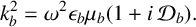 $$ \begin{align*} k_b ^2 = \omega^2\epsilon_b \mu_b (1 + i \, {\cal D}_b ). \end{align*} $$
The dissipation
 ${\cal D}_b = \sigma _b/(\omega \epsilon _b)$
is the magnitude of the conduction current density divided by the magnitude of the displacement current density [Reference Lorrain, Corson and Lorrain10] in bauxite.
${\cal D}_b = \sigma _b/(\omega \epsilon _b)$
is the magnitude of the conduction current density divided by the magnitude of the displacement current density [Reference Lorrain, Corson and Lorrain10] in bauxite.
The real part of
 $k_b$
may be written in the form [Reference Lorrain, Corson and Lorrain10, Section 11.3.1]
$k_b$
may be written in the form [Reference Lorrain, Corson and Lorrain10, Section 11.3.1]
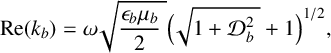 $$ \begin{align*} \operatorname{Re} (k_b) = \omega \sqrt{ \frac{\epsilon_b \mu_b }{2} \; } \Big ( \sqrt{1 + {\cal D}_b^2 \; } + 1 \Big )^{1/2} ,\end{align*} $$
while the imaginary part is
 $$ \begin{align*} \operatorname{Im} (k_b) = \omega \sqrt{ \frac{\epsilon_b \mu_b }{2} \; } \Big ( \sqrt{1 + {\cal D}_b^2 \; } - 1 \Big )^{1/2} .\end{align*} $$
The choices of plus or minus in (1.6) correspond to waves travelling in the positive and negative x directions when combined with the time dependence
 $e^{-i \omega t}$
. The wave travelling upwards in the bauxite is attenuated as it moves away from origin, so that its amplitude reduces as x increases above zero. The other wave grows in magnitude as x increases. The usual assumption in this simple model is that
$e^{-i \omega t}$
. The wave travelling upwards in the bauxite is attenuated as it moves away from origin, so that its amplitude reduces as x increases above zero. The other wave grows in magnitude as x increases. The usual assumption in this simple model is that
 $E_- = 0$
so that the electric field
$E_- = 0$
so that the electric field
 $E(x)$
does not grow without limit as x increases. This is a modelling choice to consider the bauxite to be of infinite height, and to use
$E(x)$
does not grow without limit as x increases. This is a modelling choice to consider the bauxite to be of infinite height, and to use
 $E(h)$
with h the current measured height of the bauxite as a measure of the electric field at the receiving antenna. It is also a choice that does not allow any signal reflection at interfaces, for example, between bauxite and air.
$E(h)$
with h the current measured height of the bauxite as a measure of the electric field at the receiving antenna. It is also a choice that does not allow any signal reflection at interfaces, for example, between bauxite and air.
Attenuation (reduction in electric wave amplitude with h) is then given in decibels by (1.2) for this simple model as
 $$ \begin{align*} L_s = -20 \log _{10} \bigg | \frac{E(h)}{E(0)} \bigg | = -20 \log _{10} e^{- \operatorname{Im} (k_b) h} = 20 \log _{10} (e) \operatorname{Im} (k_b) h. \end{align*} $$
For silts, dissipation
 ${\cal D} \approx 0.01$
so anticipating that dissipation is also much less than one for bauxite, it follows that
${\cal D} \approx 0.01$
so anticipating that dissipation is also much less than one for bauxite, it follows that
 $\operatorname {Im} (k_b) \approx \sqrt { \epsilon _b \mu _b}\; {\cal D}_b \omega /2$
and the attenuation is approximated for the simple model as
$\operatorname {Im} (k_b) \approx \sqrt { \epsilon _b \mu _b}\; {\cal D}_b \omega /2$
and the attenuation is approximated for the simple model as
 $$ \begin{align} L_s \approx 10 \log _{10} (e) \bigg ( \sigma_b \sqrt{ \frac{ \mu_b}{\epsilon_b}\,}\, \bigg ) h. \end{align} $$
The coefficient of h in (1.7) depends on moisture content through the effects of moisture on conductivity
 $\sigma _b$
and permittivity
$\sigma _b$
and permittivity
 $\epsilon _b$
. These effects may be nonlinear, but for small enough variations in moisture content, they will be approximately linear in moisture content. Furthermore, if moisture is almost constant, (1.7) says that attenuation is linear in h, which is wildly at odds with the data obtained for attenuation or signal strength from the microwave analyser and plotted in Figure 1. This inconsistency between measured signal strength and linear model results raises an issue with the formula used by the microwave analyser to infer moisture content from attenuation.
$\epsilon _b$
. These effects may be nonlinear, but for small enough variations in moisture content, they will be approximately linear in moisture content. Furthermore, if moisture is almost constant, (1.7) says that attenuation is linear in h, which is wildly at odds with the data obtained for attenuation or signal strength from the microwave analyser and plotted in Figure 1. This inconsistency between measured signal strength and linear model results raises an issue with the formula used by the microwave analyser to infer moisture content from attenuation.
The phase shift predicted by this simple model for small dissipation is
 $$ \begin{align*} \Delta \theta = \arg \bigg (\frac{E(h)}{E(0)} \bigg ) = \operatorname{Re} (k_b) h \approx \omega \sqrt{ \epsilon_b \mu_b \,} \,h. \end{align*} $$
This prediction of a linear dependence of phase shift on bauxite height h, with slope varying with moisture content, is consistent with the appearance of phase shift versus h seen from the data in Figure 1. It is also consistent with the formula used by the microwave analyser to predict moisture content.
These observations led the ESGI to recommend only using phase shift to infer moisture content. However, they left unresolved the question of why the attenuation data oscillate dramatically with h, beyond speculating that wave interference due to multiple internal reflections in the bauxite might be causing the issue.
1.4 Reflections
Our aim is an improved model of the travelling electromagnetic waves in the microwave analyser between transmitting and receiving antenna, as they pass through intervening air and bauxite regions. We will use the differential equations (1.5) arising from Maxwell’s equations to describe these waves.
The literature on travelling microwaves in granular material often leverages an equivalence to transmission line theory [Reference Collier4], and the branch relevant to the present application is referred to as free-space measurement of dielectric properties, in which plane microwaves are transmitted across an air gap to pass through a sample of known thickness and density before crossing another air gap to a receiving antenna [Reference Kraszewski and Kulinski8, Reference Nelson14, Reference Trabelsi and Nelson18].
Engineering electromagnetics texts such as that of Ulaby [Reference Ulaby20] show the equivalence of travelling electromagnetic waves in free space and in homogeneous media to the waves in transmission line theory, including the case of propagation through a slab [Reference Ulaby20, page 318]. However, the analysis is typically restricted to considerations like the critical thickness that makes a slab transparent.
There is good work on reflections within a single slab from the perspective of the shielding efficiency of planar materials [Reference Vojtech, Neruda and Hajek22]. In that paper, transmission through a slab of material of given thickness is modelled, with air above and below. Continuity conditions at the two interfaces are applied to solutions to correctly recover transmission and reflection terms. If we used their slab model, we would account for all reflections inside the bauxite. This would yield damped oscillations in signal strength versus h, with one wavelength that depended on bauxite properties. However, undamped reflections between bauxite and upper receiving antenna are also expected to occur within an air region which has a thickness that varies with bauxite height h. A model that combines the effects of reflection in bauxite and reflection in the overlying air gap may yield solutions that look more like our signal strength data in Figure 1, which exhibits two or more different wavelengths when plotted against h. Hence, we develop a model that allows for reflections in both the bauxite and the overlying air gap.
In the remainder of this paper, we present a new four-layer model, air–bauxite–air– antenna, that captures the effects of multiple reflections within and above the bauxite. Using this model, we solve the four resulting coupled second-order differential equations for electric field strength and associated boundary or continuity conditions for all reflection and transmission coefficients, to find an expression for the electric signal at the receiving antenna. In this way, we capture the effects of an infinite number of reflections within the variable bauxite and air layers. We will also need to use ancillary models that relate bauxite mixture properties to moisture content. Our solution provides improved matches to our signal strength data, increases our understanding of the analyser behaviour and leads to recommendations for improved moisture measurements of conveyor materials using microwave technology.
2 Four-layer model
We now develop a four-layer model, in which microwaves transmitted by the lower antenna travel through an air gap below the bauxite layer, then through a bauxite layer of variable height h, to cross another air gap before detection by a receiving antenna. The geometry is illustrated with the four numbered regions in order of increasing x, air, bauxite, air and conductor, in Figure 2, with microwaves assumed to travel in the x-direction normal to planar air/bauxite and air/antenna interfaces. Changes in bauxite height occur on a time scale of seconds, much slower than the speed of the microwaves.

Figure 2 Sketch of four-layer model, showing regions 1–4. The bauxite layer extends from
 $x=0$
to the variable height
$x=0$
to the variable height
 $x=h$
, and the air layer between bauxite and upper antenna extends from
$x=h$
, and the air layer between bauxite and upper antenna extends from
 $x=h$
to a fixed location
$x=h$
to a fixed location
 $x=D$
.
$x=D$
.
We assume the fields incident upon the base of the bauxite are free space plane waves. The transmitting antenna emits a combination of electric and magnetic fields that vary with distance in the near-field in a complicated fashion, which decrease with an inverse dependence on distance that changes from cubic to quadratic to linear, at distances much less than
 $\lambda /(2 \pi )$
from the antenna, where
$\lambda /(2 \pi )$
from the antenna, where
 $\lambda $
is the wavelength of the microwave radiation in air. The electromagnetic fields are close to free space propagation fields with constant amplitudes in the far-field at distances greater than
$\lambda $
is the wavelength of the microwave radiation in air. The electromagnetic fields are close to free space propagation fields with constant amplitudes in the far-field at distances greater than
 $\lambda /(2 \pi )$
[Reference Lorrain, Corson and Lorrain10]. For the frequency
$\lambda /(2 \pi )$
[Reference Lorrain, Corson and Lorrain10]. For the frequency
 $f=$
900 MHz used in the analyser, the wavelength is approximately 333 mm, using
$f=$
900 MHz used in the analyser, the wavelength is approximately 333 mm, using
 $\lambda = c/f$
, where the speed of light is
$\lambda = c/f$
, where the speed of light is
 $c \approx 3\times 10^8$
m/s.
$c \approx 3\times 10^8$
m/s.
Then a far-field assumption is plausible when the bauxite begins at distances at or greater than approximately 55 mm from the transmitting antenna. This requirement is taken to be met by the analyser setup, as the distances from antenna wires to the base of the conveyor belt are at least 45 mm, and in practice appear to be close to 100 mm.
Then, in region 1, we have plane wave solutions
 $$ \begin{align*} \mathbf{H}_1 & = ( 0, H_1(x)e^{-i\omega t}, 0 ), \\ \mathbf{E}_1 &= ( 0, 0, E_1(x) e^{-i \omega t} ), \end{align*} $$
where
 $E_1(x)$
satisfies the differential equation
$E_1(x)$
satisfies the differential equation
 $$ \begin{align} \frac{\partial ^2 E_1}{\partial x^2} =-\mu_0 \omega^2 \epsilon_0 E_1 , \end{align} $$
and
 $H_1$
satisfies the same equation as
$H_1$
satisfies the same equation as
 $E_1$
. Fundamental solutions take the form
$E_1$
. Fundamental solutions take the form
 $$ \begin{align*}e^{\pm ikx} ,\\[-24pt] \end{align*} $$
and substitution into (2.1) gives
 $$ \begin{align*} k^2 = \omega^2 \epsilon_0 \mu_0 = \frac{\omega^2}{c^2} , \end{align*} $$
where k is the wavenumber in free space or air, for which
 $k=2\pi /\lambda $
and
$k=2\pi /\lambda $
and
 $\lambda $
is the wavelength in free space. Without loss of generality, we choose
$\lambda $
is the wavelength in free space. Without loss of generality, we choose
 $k=\omega /c = \omega \sqrt {\epsilon _0 \mu _0 }$
. The impedance
$k=\omega /c = \omega \sqrt {\epsilon _0 \mu _0 }$
. The impedance
 $Z_0 = \mu _0 \omega /k = k/(\omega \epsilon _0) = \sqrt {\mu _0/\epsilon _0} \approx 377$
ohms will be a useful combination of parameter values.
$Z_0 = \mu _0 \omega /k = k/(\omega \epsilon _0) = \sqrt {\mu _0/\epsilon _0} \approx 377$
ohms will be a useful combination of parameter values.
The general solution is a linear combination of the two fundamental solutions. One (
 $e^{ikx}$
) corresponds to a wave travelling in the positive x-direction, and is called the incident wave. The other is a reflected wave travelling in the negative x-direction in region 1.
$e^{ikx}$
) corresponds to a wave travelling in the positive x-direction, and is called the incident wave. The other is a reflected wave travelling in the negative x-direction in region 1.
The wave in the air in region 1 where
 $x \leqslant 0 $
that is incident upon the bauxite is given by
$x \leqslant 0 $
that is incident upon the bauxite is given by
 $$ \begin{align}\begin{aligned} \mathbf{H}_i &= ( 0, e^{ikx-i\omega t}, 0 ),\\ \mathbf{E}_i &= ( 0, 0, - Z_0 e^{ikx-i \omega t} ). \end{aligned}\end{align} $$
Without loss of generality, we take the amplitude of the incident magnetic field
 $\mathbf {H}_i$
to be one in value. Other terms are in essence normalized by it. The amplitude of the electric field in (2.2) follows from Maxwell’s equation (1.3d). In region 1, there are no polarisers and the free current density is zero, so (1.3d) may be written in the form
$\mathbf {H}_i$
to be one in value. Other terms are in essence normalized by it. The amplitude of the electric field in (2.2) follows from Maxwell’s equation (1.3d). In region 1, there are no polarisers and the free current density is zero, so (1.3d) may be written in the form
 $\nabla \times \mathbf {H} = -i \omega \epsilon _0 \mathbf {E}$
, and this leads to the
$\nabla \times \mathbf {H} = -i \omega \epsilon _0 \mathbf {E}$
, and this leads to the
 $Z_0$
term in (2.2). In region 1, the reflected wave is of unknown amplitude R, and is given by
$Z_0$
term in (2.2). In region 1, the reflected wave is of unknown amplitude R, and is given by
 $$ \begin{align*} \mathbf{H}_r &= ( 0, Re^{-ikx-i\omega t}, 0 ), \\ \mathbf{E}_r &= ( 0, 0, R Z_0 e^{-ikx-i\omega t} ). \end{align*} $$
In region 2, where
 $0 \leqslant x \leqslant h$
, the waves are travelling through the bauxite mixture with fields described as in Section 1.3 by
$0 \leqslant x \leqslant h$
, the waves are travelling through the bauxite mixture with fields described as in Section 1.3 by
 $$ \begin{align*} \mathbf{H} = ( 0, H(x), 0 ) e^{-i\omega t} , \quad \mathbf{E} = ( 0, 0, E(x) ) e^{-i \omega t} , \end{align*} $$
with solutions for
 $E(x)$
 $$ \begin{align} E = E_+ e^{ i k_b x} + E_- e^{- i k_b x}. \end{align} $$
The amplitudes
 $E_+$
and
$E_+$
and
 $E_-$
of the upwards and downwards travelling waves will be determined by applying boundary conditions. Note that this approach allows for reflections at air/bauxite interfaces, in contrast to the approach taken in Section 1.3.
$E_-$
of the upwards and downwards travelling waves will be determined by applying boundary conditions. Note that this approach allows for reflections at air/bauxite interfaces, in contrast to the approach taken in Section 1.3.
In the air in region 3, where
 $h \leqslant x \leqslant D$
, there is a transmitted wave travelling upwards of unknown amplitude T given by
$h \leqslant x \leqslant D$
, there is a transmitted wave travelling upwards of unknown amplitude T given by
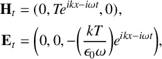 $$ \begin{align*} \mathbf{H}_t &= ( 0, Te^{ikx-i\omega t}, 0 ) , \\ \mathbf{E}_t &= \bigg ( 0, 0, - \bigg (\frac{kT}{\epsilon_0 \omega}\bigg )e^{ikx-i \omega t} \bigg ) , \end{align*} $$
and a reflected wave coming back from the receiving antenna, of unknown amplitude
 $R_2$
:
$R_2$
:
 $$ \begin{align*} \mathbf{H}_{r2} &= ( 0, R_2 e^{-ikx-i\omega t}, 0 ) , \\ \mathbf{E}_{r2} &= \bigg ( 0, 0, \bigg (\frac{kR_2 }{\epsilon_0 \omega}\bigg )e^{-ikx-i \omega t} \bigg ). \end{align*} $$
In region 4, the receiving antenna will be modelled as a semi-infinite material with relatively high electrical conductivity, with the analyser signal that provides our data assumed to be drawn from an antenna that is at the surface of that material at
 $x=D$
. In the antenna region
$x=D$
. In the antenna region
 $x \geqslant D$
, we have the fields
$x \geqslant D$
, we have the fields
 $$ \begin{align*} \mathbf{H}_a & = (0,H_a(x) , 0) e^{-i \omega t} , \\ \mathbf{E}_a & =(0,0, E_a(x) ) e^{-i \omega t}. \end{align*} $$
In the antenna, (1.5) applies but with the effective properties of the antenna material indicated by subscripts a, so that
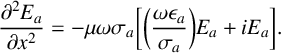 $$ \begin{align} \frac{\partial ^2 E_a}{\partial x^2} =-\mu \omega \sigma_a \bigg [ \bigg (\frac{\omega \epsilon_a}{\sigma_a} \bigg ) E_a + i E_a \bigg ]. \end{align} $$
The general solution to (2.4) can be written as
 $$ \begin{align*} E_a = A_+ e^{ i k_a (x-D)} + A_- e^{- i k_a (x-D)}. \end{align*} $$
Substitution of this solution into (2.4) requires that the wavenumber
 $k_a$
in the antenna satisfies the equation
$k_a$
in the antenna satisfies the equation
 $$ \begin{align*} k_a ^2 = \omega^2\epsilon_a \mu \bigg (1 + i \frac{\sigma_a}{\omega \epsilon_a} \bigg ) , \end{align*} $$
and the constants
 $A_\pm $
are to be determined. The electromagnetic properties of the receiving antenna are not known to us. They could be chosen to be those of an almost lossless 50 ohm transmission line. Choosing the root
$A_\pm $
are to be determined. The electromagnetic properties of the receiving antenna are not known to us. They could be chosen to be those of an almost lossless 50 ohm transmission line. Choosing the root
 $k_a$
without loss of generality to be the one with positive imaginary part, vanishing of
$k_a$
without loss of generality to be the one with positive imaginary part, vanishing of
 $E_a$
as
$E_a$
as
 $x \to \infty $
requires that
$x \to \infty $
requires that
 $A_- = 0$
.
$A_- = 0$
.
There are three unknown transmission and reflection coefficients R, T and
 $R_2$
, plus two unknown amplitudes
$R_2$
, plus two unknown amplitudes
 $E_+$
and
$E_+$
and
 $E_-$
in the bauxite, and the remaining unknown coefficient
$E_-$
in the bauxite, and the remaining unknown coefficient
 $A_+$
in the receiving antenna. These six unknown constants are provided by three pairs of boundary conditions which give six linear equations that are to be solved simultaneously.
$A_+$
in the receiving antenna. These six unknown constants are provided by three pairs of boundary conditions which give six linear equations that are to be solved simultaneously.
The pair at
 $x=0$
is given as follows. Continuity of the tangential component of
$x=0$
is given as follows. Continuity of the tangential component of
 $\mathbf {H}$
gives
$\mathbf {H}$
gives
 $ H(0) = 1+R $
. In the bauxite, Maxwell’s equation (1.3c) gives
$ H(0) = 1+R $
. In the bauxite, Maxwell’s equation (1.3c) gives
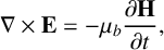 $$ \begin{align*}\nabla \times \mathbf{E} = - \mu_b \frac{\partial \mathbf{H}}{\partial t}, \end{align*} $$
so that
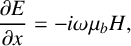 $$ \begin{align} \frac{\partial E}{\partial x} = -i \omega \mu_b H , \end{align} $$
and then
 $$ \begin{align} \frac{\partial E}{\partial x} = -i \mu_b \omega (1+R). \end{align} $$
Continuity of the tangential component of
 $\mathbf {E}$
directly gives
$\mathbf {E}$
directly gives
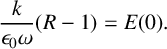 $$ \begin{align} \frac{k}{\epsilon_0 \omega}(R-1) = E(0). \end{align} $$
The pair at
 $x=h$
is given in a similar manner. Continuity of
$x=h$
is given in a similar manner. Continuity of
 $\mathbf {H} \times \mathbf {n}$
gives
$\mathbf {H} \times \mathbf {n}$
gives
 $H(h)= T e^{ikh} + R_2 e^{-ikh} $
, so that (2.5) yields
$H(h)= T e^{ikh} + R_2 e^{-ikh} $
, so that (2.5) yields
 $$ \begin{align} \frac{\partial E}{\partial x} = -i \mu_b \omega ( T e^{ikh} + R_2 e^{-ikh} ) , \end{align} $$
and continuity of
 $\mathbf {E} \times \mathbf {n}$
yields
$\mathbf {E} \times \mathbf {n}$
yields
 $$ \begin{align} E(h) = - \bigg ( \frac{k}{\epsilon_0 \omega} \bigg ) ( Te^{ikh} - R_2 e^{-ikh} ). \end{align} $$
At the antenna
 $x=D$
, continuity of
$x=D$
, continuity of
 $\mathbf {H} \times \mathbf {n}$
gives
$\mathbf {H} \times \mathbf {n}$
gives
 $H_a= T e^{ikD} + R_2 e^{-ikD} $
, so that (2.5) (but using antenna properties) gives
$H_a= T e^{ikD} + R_2 e^{-ikD} $
, so that (2.5) (but using antenna properties) gives
 $$ \begin{align} \frac{\partial E_a}{\partial x} = -i \mu_0 \omega ( Te^{ikD} + R_2 e^{-ikD} ) , \end{align} $$
and continuity of
 $\mathbf {E} \times \mathbf {n}$
gives
$\mathbf {E} \times \mathbf {n}$
gives
 $$ \begin{align} E_a (D) = - \bigg ( \frac{k}{\epsilon_0 \omega} \bigg ) ( Te^{ikD} - R_2 e^{-ikD} ). \end{align} $$
It is helpful to set up the boundary conditions as a matrix problem to be solved for the six unknowns
 $E_+$
,
$E_+$
,
 $E_-$
, R, T,
$E_-$
, R, T,
 $R_2$
and
$R_2$
and
 $A_+$
. We are particularly interested in finding
$A_+$
. We are particularly interested in finding
 $A_+$
, giving us the signal in the receiving antenna. Equations (2.6) and (2.7) give
$A_+$
, giving us the signal in the receiving antenna. Equations (2.6) and (2.7) give
 $$ \begin{align} E_+ + E_- - Z_0 R &= - Z_0 , \end{align} $$
 $$ \begin{align} E_+ - E_- + Z_b R &= - Z_b , \end{align} $$
where
 $Z_b = \mu _b \omega / k_b $
is the impedance of the bauxite mixture. Equations (2.8) and (2.9) together with (2.3) give
$Z_b = \mu _b \omega / k_b $
is the impedance of the bauxite mixture. Equations (2.8) and (2.9) together with (2.3) give
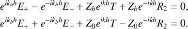 $$ \begin{align*} e^{ik_b h} E_+ - e^{-ik_b h}E_- + Z_b e^{ikh} T + Z_b e^{-ikh} R_2 &= 0 , \\ e^{ik_b h} E_+ + e^{-ik_b h}E_- + Z_0 e^{ikh} T - Z_0 e^{-ikh} R_2 &= 0. \end{align*} $$
Equations (2.10) and (2.11) together with
 $E_a = A_+ e^{ i k_a (x-D)} $
give
$E_a = A_+ e^{ i k_a (x-D)} $
give
 $$ \begin{align} Z_a e^{ik D}T + Z_a e^{-ik D}R_2 + A_+ &= 0 , \end{align} $$
 $$ \begin{align} Z_0 e^{ik D}T - Z_0 e^{-ik D}R_2 + A_+ &= 0 , \end{align} $$
where
 $Z_a = \mu _0 \omega / k_a$
is the impedance of the region representing the receiving antenna. Then (2.12)–(2.15) can be written in matrix form:
$Z_a = \mu _0 \omega / k_a$
is the impedance of the region representing the receiving antenna. Then (2.12)–(2.15) can be written in matrix form:
 $$ \begin{align*} \left ( \begin{array}{cccccc} 1, & 1, & -Z_0, & 0, & 0, & 0 \\ 1, & -1, & Z_b, & 0, & 0, & 0 \\ e^{i k_b h} , & -e^{-i k_b h} , & 0,& Z_b e^{i k h} , & Z_b e^{-i k h} , & 0\\ e^{i k_b h} , & e^{-i k_b h} , & 0,& Z_0 e^{i k h} , & -Z_0 e^{-i k h} , & 0\\ 0,&0,&0,&Z_a e^{i k D} , & Z_a e^{-i k D}, & 1 \\ 0,&0,&0,&Z_0 e^{i k D} , & -Z_0 e^{-i k D}, & 1 \\ \end{array} \right ) \left ( \begin{array}{c} E_+\\ E_- \\ R \\ T \\ R_2 \\ A_+ \end{array} \right ) = \left ( \begin{array}{c } -Z_0\\ -Z_b \\ 0 \\ 0 \\ 0 \\ 0 \end{array} \right ) , \end{align*} $$
and represented as the augmented matrix
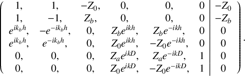 $$ \begin{align*} \left ( \begin{array}{cccccc|c} 1, & 1, & -Z_0, & 0, & 0, & 0 & -Z_0\\ 1, & -1, & Z_b, & 0, & 0, & 0 & -Z_b\\ e^{i k_b h} , & -e^{-i k_b h} , & 0,& Z_b e^{i k h} , & Z_b e^{-i k h} , & 0& 0\\ e^{i k_b h} , & e^{-i k_b h} , & 0,& Z_0 e^{i k h} , & -Z_0 e^{-i k h} , & 0& 0\\ 0,&0,&0,&Z_a e^{i k D} , & Z_a e^{-i k D}, & 1 & 0\\ 0,&0,&0,&Z_0 e^{i k D} , & -Z_0 e^{-i k D}, & 1 & 0 \end{array} \right ). \end{align*} $$
Gauss–Jordan row reduction gives an upper triangular augmented matrix which allows to read off the solutions
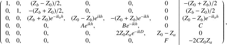 $$ \begin{align*} \left ( \begin{array}{cccccc|c} 1, & 0, & (Z_b-Z_0)/2, & 0, & 0, & 0 & -(Z_0+Z_b)/2\\ 0, & 1, & -(Z_b+Z_0)/2, & 0, & 0, & 0 & (Z_b-Z_0)/2\\ 0 , & 0 , & (Z_b + Z_0)e^{-ik_bh},& (Z_0-Z_b) e^{i k h} , & -(Z_0+Z_b) e^{-i k h} , & 0& (Z_0-Z_b)e^{-ik_bh}\\ 0 , & 0 , & 0,& Ae^{ikh} , & B e^{-i k h} , & 0& C\\ 0,&0,&0,&0 , & 2Z_0 Z_a e^{-i k D}, & Z_0-Z_a & 0\\ 0,&0,&0,&0 , & 0, & F & -2C Z_0 Z_a \end{array} \right ) , \end{align*} $$
where
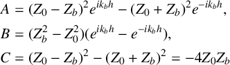 $$ \begin{align*} A &= (Z_0-Z_b)^2 e^{i k_b h} - (Z_0+Z_b)^2 e^{-i k_b h} , \\ B &= (Z_b^2 - Z_0^2) (e^{i k_b h} - e^{-i k_b h} ) , \\ C & = (Z_0-Z_b)^2 - (Z_0 + Z_b)^2 = -4 Z_0 Z_b \end{align*} $$
and
 $$ \begin{align*}F = B (Z_0 - Z_a) e^{ik(D-h)} + A (Z_0+Z_a) e^{-ik(D-h)} .\end{align*} $$
It follows that the signal at the surface of the receiving antenna is
 $$ \begin{align} A_+ = -\frac{ 2C Z_0 Z_a}{F}. \end{align} $$
Note that F depends on
 $k(D-h)$
, and through A and B, it depends also on
$k(D-h)$
, and through A and B, it depends also on
 $k_b h$
, giving two different wavelengths versus h, one determined by free-space properties in the real part of k and the other by bauxite properties in the real part of
$k_b h$
, giving two different wavelengths versus h, one determined by free-space properties in the real part of k and the other by bauxite properties in the real part of
 $k_b$
.
$k_b$
.
The other unknowns can now be computed by back-substitution, for example, row 5 now gives
 $$ \begin{align*}2 Z_0 Z_a e^{-i k D}R_2 + (Z_0-Z_a)A_+ = 0,\end{align*} $$
so that
 $$ \begin{align*} R_2 = \frac{ C}{F} (Z_0-Z_a) e^{i k D}. \end{align*} $$
A simple way to obtain (2.16) for
 $A_+$
(and all of the other unknowns) is to use MATLAB’s command
$A_+$
(and all of the other unknowns) is to use MATLAB’s command
syms Z0 Za Zb k kb h D
to set up symbols for each term in the matrix, then use the rref command on the augmented symbolic matrix to return the reduced row echelon form using Gauss–Jordan elimination with partial pivoting. The returned solution components are in symbolic form, and are expanded-out versions of what is obtained by hand above. They provided us with a useful check against errors in our hand calculations.
Other forms for
 $A_+$
are
$A_+$
are
 $$ \begin{align*} A_+ = \frac{ 8 Z_0^2 Z_a Z_b \; e^{ikD} e^{ikh} e^{ik_b h}}{F_2} , \end{align*} $$
where
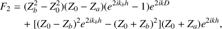 $$ \begin{align} F_2 &= (Z_b^2 - Z_0^2)(Z_0-Z_a) ( e^{2ik_b h} - 1 ) e^{2ikD} \nonumber \\ & \quad+ [ (Z_0-Z_b)^2 e^{2i k_b h} - (Z_0+Z_b)^2 ](Z_0 + Z_a) e^{2ikh} , \end{align} $$
and
 $$ \begin{align*} A_+ = \frac{ 2 (1-R_\infty) Z_0Z_a}{(Z_0+Z_a)F_3} , \end{align*} $$
where
 $$ \begin{align*} F_3 = R_a R_\infty ( e^{-ik_b h} - e^{ik_b h} ) e^{ik(D-h)} + ( R_\infty ^2 e^{i k_b h} - e^{-i k_b h} ) e^{-ik(D-h)} \end{align*} $$
and
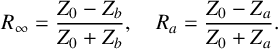 $$ \begin{align}R_\infty = \frac{Z_0-Z_b}{Z_0+Z_b} , \quad R_a = \frac{Z_0-Z_a}{Z_0+Z_a}. \end{align} $$
The term labelled
 $R_\infty $
is the reflection coefficient that would apply at
$R_\infty $
is the reflection coefficient that would apply at
 $x=0$
if the bauxite height
$x=0$
if the bauxite height
 $h \to \infty $
. This standard result can be seen in our four-layer model if we set
$h \to \infty $
. This standard result can be seen in our four-layer model if we set
 $E_-$
to zero (so that there is no reflection from
$E_-$
to zero (so that there is no reflection from
 $x=h$
, or that
$x=h$
, or that
 $|E| \to 0$
in the bauxite as
$|E| \to 0$
in the bauxite as
 $h \to \infty $
), so that (2.12) and (2.13) become, after replacing R with
$h \to \infty $
), so that (2.12) and (2.13) become, after replacing R with
 $R_\infty $
,
$R_\infty $
,
 $$ \begin{align*} E_+ - Z_0 R_\infty = - Z_0 , \quad E_+ + Z_b R_\infty = - Z_b. \end{align*} $$
Now
 $E_+$
can be eliminated to give the form (2.18) for
$E_+$
can be eliminated to give the form (2.18) for
 $R_\infty $
.
$R_\infty $
.
As the bauxite height
 $h \to 0$
, it follows that
$h \to 0$
, it follows that
 $A \to C$
and
$A \to C$
and
 $B \to 0$
and
$B \to 0$
and
 $F \to C(Z_0+Z_a) e^{-ikD}$
. Then in the absence of bauxite, the magnitude of the received signal becomes, using (2.16),
$F \to C(Z_0+Z_a) e^{-ikD}$
. Then in the absence of bauxite, the magnitude of the received signal becomes, using (2.16),
 $$ \begin{align} |A_+| \to \bigg |\frac{2 Z_0 Z_a }{ Z_0+Z_a} \bigg | , \quad h \to 0. \end{align} $$
We see in (2.19) that, in general, the magnitude
 $ |A_+|$
of the received signal does not simplify to the magnitude of the transmitted electric field (
$ |A_+|$
of the received signal does not simplify to the magnitude of the transmitted electric field (
 $Z_0$
) as
$Z_0$
) as
 $h \to 0$
. This is due to the mismatch between the free-space impedance
$h \to 0$
. This is due to the mismatch between the free-space impedance
 $Z_0$
used for the transmitted wave in region 1, and the impedance
$Z_0$
used for the transmitted wave in region 1, and the impedance
 $Z_a$
of the receiving antenna. The detected power tends to the transmitted power (and attenuation tends to zero, or
$Z_a$
of the receiving antenna. The detected power tends to the transmitted power (and attenuation tends to zero, or
 $|Z_0/A_+|$
tends to one) as
$|Z_0/A_+|$
tends to one) as
 $h \to 0$
only in the unrealistic case that the impedance
$h \to 0$
only in the unrealistic case that the impedance
 $Z_a$
of the receiving antenna is matched to
$Z_a$
of the receiving antenna is matched to
 $Z_0$
.
$Z_0$
.
The impact of bauxite and its attendant moisture on the analyser setup is naturally measured by using, say (2.16), to provide the zero bauxite value for the response of the receiving antenna as the reference signal,
 $$ \begin{align*}A_+ ^0 = \lim _{h \to 0} A_+ = - \bigg ( \frac{2 Z_0 Z_a}{Z_0+Z_a}\bigg ) e^{ikD} ,\end{align*} $$
which captures the instrumental effect of mismatched impedances between transmitting and receiving antennae. Then using (2.16) again, the dependence of
 $A_+$
on h relative to the zero bauxite value
$A_+$
on h relative to the zero bauxite value
 $A_+ ^0$
is given by
$A_+ ^0$
is given by
 $$ \begin{align*} A^0_{\tt4L} = 20 \log_{10} \bigg | \frac{A_+ ^0}{A_+} \bigg | = 20 \log_{10} \bigg | \frac{F}{C(Z_0+Z_a)} \bigg |. \end{align*} $$
This provides the decibel measure of attenuation due to the presence of bauxite mixture on the belt, and is zero in the limit
 $h \to 0$
.
$h \to 0$
.
The attenuation then depends on bauxite thickness h via exponents involving
 $ikh$
and
$ikh$
and
 $ik_b h$
, that is, combinations of sinusoids with magnitudes that have wavelengths
$ik_b h$
, that is, combinations of sinusoids with magnitudes that have wavelengths
 $ \pi /k \approx $
166 mm and
$ \pi /k \approx $
166 mm and
 $\pi / \operatorname {Re}(k_b) \approx $
30–80 mm (using damp silt properties).
$\pi / \operatorname {Re}(k_b) \approx $
30–80 mm (using damp silt properties).
The terms appearing in (2.17), which forms part of the detected electric field
 $A_+$
, involve
$A_+$
, involve
 $e^{2ik_bh}$
and
$e^{2ik_bh}$
and
 $e^{2ikh}$
, indicating that reflections cause the observed oscillations to have half the wavelengths of travelling waves without reflections present.
$e^{2ikh}$
, indicating that reflections cause the observed oscillations to have half the wavelengths of travelling waves without reflections present.
That is, our four-layer model predicts wavelengths of 83 mm and 15–40 mm, consistent with what is seen in the graph of signal strength data versus h in Figure 1. The longer wavelength is associated with reflections occurring in region 3 above the bauxite, while the shorter is associated with reflections occurring inside the bauxite in region 2.
A simple physical explanation that ignores attenuation for reflections within the bauxite slab causing constructive interference effects with wavelengths that are half of those of the travelling wave can be made. The first and largest reflected wave travels a distance
 $3h$
compared with a nonreflected wave travelling a distance h. Adding sinusoids
$3h$
compared with a nonreflected wave travelling a distance h. Adding sinusoids
 $\sin (kh) +\sin ({3kh})$
gives a term depending on
$\sin (kh) +\sin ({3kh})$
gives a term depending on
 $2kh$
from the sin sum formula, that is, half the wavelength of a
$2kh$
from the sin sum formula, that is, half the wavelength of a
 $kh$
term.
$kh$
term.
The signal strength data from the analyser are to be compared with our four-layer model prediction,
 $$ \begin{align*} SS = -A^0_{\tt4L} = - 20 \log_{10} \bigg | \frac{A_+ ^0}{A_+} \bigg | = 20 \log_{10} \bigg | \frac{A_+ }{A_+^0} \bigg | , \end{align*} $$
and the phase shift data derived from analyser output [Reference McGuinness, Bohun, Cregan, Lee, Dewynne, O’Keeffe, Vo, McKibbin, Wake and Saeki12] are to be compared with our model
 $$ \begin{align*} \Delta \phi = {\tt angle} \bigg ( \frac{A_+ }{A_+^0} \bigg ) .\end{align*} $$
Important parameters are the distance D between the upper antenna and the unloaded conveyor belt, the permittivity
 $\epsilon _r$
and the electric conductivity
$\epsilon _r$
and the electric conductivity
 $\sigma _b$
of the bauxite mixture. We now compare the behaviour of our four-layer model to the data from the microwave analyser.
$\sigma _b$
of the bauxite mixture. We now compare the behaviour of our four-layer model to the data from the microwave analyser.
3 Results
We examine the effects of three important parameters D,
 $\epsilon _r$
and
$\epsilon _r$
and
 $\sigma $
on the solution to our model, while comparing with data.
$\sigma $
on the solution to our model, while comparing with data.
3.1 Distance
 $\boldsymbol {D}$

The ranges of D values investigated were chosen after studying technical drawings of the microwave analyser, which give the distance between the inner surfaces of the antenna housings as approximately 600 mm. The housings are each 120 mm thick. The drawings do not reveal the exact structure of the antennae, or where inside the housings the wires are, so there is some uncertainty in the correct value for D. We have compared model results to data to help determine an accurate value for D, and we found they are sensitive to changes in D of just a few millimetres.
We noticed that for a signal strength, smaller D values matched data from smaller bauxite heights, while larger D values did better at larger heights, suggesting conveyor belt sag might be affecting the data. Conveyor belt sag affects measured bauxite height since the ultrasound sensor is mounted above the bauxite looking down on it, so any sag means the true bauxite height is larger than measured. Sag also increases the distance D from the bottom of the bauxite to the receiving antenna, making it a function of h. We found improved matches to signal strength data when we adjusted original data heights
 $h_0$
to a true height h using
$h_0$
to a true height h using
 $$ \begin{align*} h = h_0 + {\tt sag}, \end{align*} $$
and we used in our model
 $$ \begin{align*} D = D_0 + {\tt sag}, \end{align*} $$
where
 $D_0$
is the distance from empty belt to receiving antenna, and where
$D_0$
is the distance from empty belt to receiving antenna, and where
 $$ \begin{align*} {\tt sag} = \frac{S_m}{\pi} ( \arctan ((h-h_0)/S_e) + \arctan (h_0/S_e) ) \end{align*} $$
with maximum sag
 $S_m = 0.1$
m, centre of sag
$S_m = 0.1$
m, centre of sag
 $h_0=0.25$
m and extent
$h_0=0.25$
m and extent
 $S_e=0.05$
m. The resulting sag values and adjusted height values are illustrated in Figure 3.
$S_e=0.05$
m. The resulting sag values and adjusted height values are illustrated in Figure 3.

Figure 3 Conveyor belt sag used to improve matches between data and our four-layer model. The effect of the sag on measured bauxite heights is illustrated in the right-hand plot. The dashed line indicates zero sag values and the solid line shows height values corrected for sag.
We compute signal strength and phase shift for a range of values for the distance
 $D_0$
and, as illustrated in Figure 4, the model signal strength is very sensitive to this distance, as it strongly affects the interference effect in region 3 between bauxite and receiving antenna. Changes of just 5 mm in
$D_0$
and, as illustrated in Figure 4, the model signal strength is very sensitive to this distance, as it strongly affects the interference effect in region 3 between bauxite and receiving antenna. Changes of just 5 mm in
 $D_0$
have a significant effect on signal strength when plotted against h. Good matches to signal strength are seen with 70 mm maximum belt sag but the phase shift data do not give a good match to the model when this much belt sag is used. We also see that phase shift is much less sensitive to changes in
$D_0$
have a significant effect on signal strength when plotted against h. Good matches to signal strength are seen with 70 mm maximum belt sag but the phase shift data do not give a good match to the model when this much belt sag is used. We also see that phase shift is much less sensitive to changes in
 $D_0$
.
$D_0$
.

Figure 4 Comparisons of our four-layer model results with microwave analyser data, for varying values of the distance
 $D_0$
(mm) between empty belt and receiving antenna. The
$D_0$
(mm) between empty belt and receiving antenna. The
 $D_0$
values generating model results (lines) are listed in the legend and data are represented by dots. Antenna properties are taken to be
$D_0$
values generating model results (lines) are listed in the legend and data are represented by dots. Antenna properties are taken to be
 $\epsilon _a=\epsilon _0$
and
$\epsilon _a=\epsilon _0$
and
 $\sigma _a=50$
S/m, and bauxite properties are
$\sigma _a=50$
S/m, and bauxite properties are
 $\epsilon _r =6.5$
and
$\epsilon _r =6.5$
and
 $\sigma _b=30$
mS/m. Belt sag maximum is 70 mm.
$\sigma _b=30$
mS/m. Belt sag maximum is 70 mm.
Reducing the belt sag to have a maximum of 40 mm (and reducing
 $\epsilon _r$
to a value of 6.2) leads to a better overall match, as illustrated in Figure 5, but at the expense of the signal strength match. The alignment of phase shifts at higher h values indicates that belt sag is better set to zero. The data acquired at smaller h values are relatively noisy, and are subject to timing issues as the bauxite height typically only passes briefly through these value, with approximately six values recorded each time the belt goes between unloaded and the typical full load of 200–250 mm height. So we set zero sag for the remaining model simulations in this paper, and we will use
$\epsilon _r$
to a value of 6.2) leads to a better overall match, as illustrated in Figure 5, but at the expense of the signal strength match. The alignment of phase shifts at higher h values indicates that belt sag is better set to zero. The data acquired at smaller h values are relatively noisy, and are subject to timing issues as the bauxite height typically only passes briefly through these value, with approximately six values recorded each time the belt goes between unloaded and the typical full load of 200–250 mm height. So we set zero sag for the remaining model simulations in this paper, and we will use
 $D_0 = 0.615$
.
$D_0 = 0.615$
.

Figure 5 Comparisons of our four-layer model results with microwave analyser data for varying values of the distance
 $D_0$
(mm) between empty belt and receiving antenna. The
$D_0$
(mm) between empty belt and receiving antenna. The
 $D_0$
values generating model results (lines) are listed in the legend and data are represented by dots. Antenna properties are taken to be
$D_0$
values generating model results (lines) are listed in the legend and data are represented by dots. Antenna properties are taken to be
 $\epsilon _a=\epsilon _0$
and
$\epsilon _a=\epsilon _0$
and
 $\sigma _a=50$
S/m, and bauxite properties are
$\sigma _a=50$
S/m, and bauxite properties are
 $\epsilon _r =6.2$
and
$\epsilon _r =6.2$
and
 $\sigma _b=30$
mS/m. Belt sag maximum is 40 mm.
$\sigma _b=30$
mS/m. Belt sag maximum is 40 mm.
3.2 Inferring permittivity and conductivity
We now explore implications of the four-layer model for inferring the permittivity and the electrical conductivity of the bauxite mixture from the signal strengths, phase shifts and bauxite heights provided by the microwave analyser.
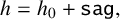
Four-layer model responses are illustrated for varying bauxite relative permittivities in Figures 6 and 7, with fixed
 $D=0.615$
m. The signal strength curves cross each other in multiple locations, in contrast to the phase shifts which look much more useful for inferring bauxite permittivity.
$D=0.615$
m. The signal strength curves cross each other in multiple locations, in contrast to the phase shifts which look much more useful for inferring bauxite permittivity.

Figure 6 Comparisons of our four-layer model results with microwave analyser data for varying values of the bauxite mixture permittivity. The
 $\epsilon _r$
values generating model results (lines) are listed in the legend and data are represented by dots. Antenna properties are taken to be
$\epsilon _r$
values generating model results (lines) are listed in the legend and data are represented by dots. Antenna properties are taken to be
 $\epsilon _a=\epsilon _0$
and
$\epsilon _a=\epsilon _0$
and
 $\sigma _a=50$
S/m, and bauxite conductivity is fixed at
$\sigma _a=50$
S/m, and bauxite conductivity is fixed at
 $\sigma _b=35$
mS/m. The distance
$\sigma _b=35$
mS/m. The distance
 $D=0.615$
m is fixed. Belt sag is zero. Signal strengths are in dB. Phase shifts are in radians.
$D=0.615$
m is fixed. Belt sag is zero. Signal strengths are in dB. Phase shifts are in radians.

Figure 7 Four-layer model results with varying values of the bauxite mixture permittivity. A simpler line style and more finely spaced permittivity values are used to make clearer the appearance of the surface, that is,
 $\epsilon _r$
as a function of signal strength and h, through its level curves. Other parameter values are the same as in Figure 6.
$\epsilon _r$
as a function of signal strength and h, through its level curves. Other parameter values are the same as in Figure 6.
The crossings of the curves of constant permittivity in the signal strength plots are indicative of noninvertible graphs of permittivity versus signal strength at given h values. That is, folds in the surface indicate where there is more than one permittivity value giving a particular value of signal strength (given h), so that the signal data cannot in general be used to infer permittivity.
This may be clearer in the visualization of the signal strength as a function of h and
 $\epsilon _r$
shown in the waterfall plot in Figure 8. Here are plotted curves of constant h, which reveal that sometimes a single data value for signal strength
$\epsilon _r$
shown in the waterfall plot in Figure 8. Here are plotted curves of constant h, which reveal that sometimes a single data value for signal strength
 $SS$
may be obtained by more than one choice of
$SS$
may be obtained by more than one choice of
 $\epsilon _r$
. This becomes clear when considering
$\epsilon _r$
. This becomes clear when considering
 $SS$
–
$SS$
–
 $\epsilon _r$
planes at a given h value, featuring curves that fail the horizontal line test for invertibility. For example, there are two choices for
$\epsilon _r$
planes at a given h value, featuring curves that fail the horizontal line test for invertibility. For example, there are two choices for
 $\epsilon _r$
near
$\epsilon _r$
near
 $h=150$
giving
$h=150$
giving
 $SS = -2$
, or three choices for
$SS = -2$
, or three choices for
 $\epsilon _r$
near
$\epsilon _r$
near
 $h=250$
giving
$h=250$
giving
 $SS = -7$
. However, model phase shifts are invertible, and do provide a single value of permittivity – at any given h, a value for phase shift is clearly associated with just one bauxite permittivity value.
$SS = -7$
. However, model phase shifts are invertible, and do provide a single value of permittivity – at any given h, a value for phase shift is clearly associated with just one bauxite permittivity value.

Figure 8 Four-layer model signal strength (
 $SS$
, in dB) results visualized as waterfall plots using two different view points. They show
$SS$
, in dB) results visualized as waterfall plots using two different view points. They show
 $SS$
as a surface, a function of h(mm) and bauxite mixture permittivity
$SS$
as a surface, a function of h(mm) and bauxite mixture permittivity
 $\epsilon _r$
. Antenna properties are taken to be
$\epsilon _r$
. Antenna properties are taken to be
 $\epsilon _a=\epsilon _0$
and
$\epsilon _a=\epsilon _0$
and
 $\sigma _a=50$
S/m, and bauxite conductivity is fixed at
$\sigma _a=50$
S/m, and bauxite conductivity is fixed at
 $\sigma _b=35$
mS/m.
$\sigma _b=35$
mS/m.
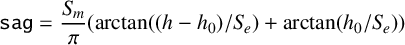
The four-layer model responses as the bauxite mixture electric conductivity is varied are illustrated in Figure 9, with fixed
 $D=0.615$
m. The signal strength curves now look much more useful for inferring bauxite conductivity, if permittivity is constant. The phase shifts however are very insensitive to conductivity, and on close inspection, they also cross over each other as h varies.
$D=0.615$
m. The signal strength curves now look much more useful for inferring bauxite conductivity, if permittivity is constant. The phase shifts however are very insensitive to conductivity, and on close inspection, they also cross over each other as h varies.

Figure 9 Four-layer model results with varying values of the bauxite mixture conductivity. The
 $\sigma _b$
values generating model results (lines) are listed in the legend with units mS/m. Antenna properties are taken to be
$\sigma _b$
values generating model results (lines) are listed in the legend with units mS/m. Antenna properties are taken to be
 $\epsilon _a=\epsilon _0$
and
$\epsilon _a=\epsilon _0$
and
 $\sigma _a=50$
S/m, and bauxite relative permittivity is fixed at
$\sigma _a=50$
S/m, and bauxite relative permittivity is fixed at
 $\epsilon _r=7.5$
.
$\epsilon _r=7.5$
.
Recalling that measurements on silts [Reference Dobson and Ulaby5] have both relative permittivity and conductivity of the mixture increasing with moisture content, it remains unclear whether either signal strength or phase shift can be used to infer moisture content without further analysis of the relationships between moisture content and electromagnetic mixture properties. The broad implications of the modelling here are that the effects of reflections could be very unhelpful for inferring moisture content.
Changing the spacing of the antenna does not improve things at current microwave analyser settings – variations of bauxite height as the conveyor goes between empty and full are of the same order as the wavelength of the microwaves in air. Deciding to only use measurements taken near a fully loaded conveyor belt does not help, as changes in bauxite moisture at any given value of h are always dominated by reflection, overwhelming the inference of electromagnetic properties and thence moisture content.
4 Frequency reduction
Reducing the microwave operating frequency is one possible approach to improving the usefulness of the analyser, with encouraging results from our model as illustrated in Figures 10 and 11, where frequency is one-tenth of the usual analyser operating frequency. The longer wavelength of more than 3 m now means there is less interference from reflected waves over the relatively smaller distances h and
 $D-h$
.
$D-h$
.
Figure 10 Four-layer model results with frequency lowered to 0.09 GHz. The
 $\epsilon _r$
values generating signal strengths and phase shifts (lines) are listed in the legend. Antenna properties are taken to be
$\epsilon _r$
values generating signal strengths and phase shifts (lines) are listed in the legend. Antenna properties are taken to be
 $\epsilon _a=\epsilon _0$
and
$\epsilon _a=\epsilon _0$
and
 $\sigma _a=50$
S/m, and bauxite electrical conductivity is fixed at
$\sigma _a=50$
S/m, and bauxite electrical conductivity is fixed at
 $\sigma =35$
mS/m. Sag is zero.
$\sigma =35$
mS/m. Sag is zero.
Figure 11 Four-layer model results with frequency lowered to 0.09 GHz. The
 $\sigma $
values generating model results (lines) are listed in the legend. Antenna properties are taken to be
$\sigma $
values generating model results (lines) are listed in the legend. Antenna properties are taken to be
 $\epsilon _a=\epsilon _0$
and
$\epsilon _a=\epsilon _0$
and
 $\sigma _a=50$
S/m, and bauxite relative permittivity is fixed at
$\sigma _a=50$
S/m, and bauxite relative permittivity is fixed at
 $\epsilon _r=7.5$
. Sag is zero.
$\epsilon _r=7.5$
. Sag is zero.
Then signal strength variations are nicely correlated to changes in electrical conductivity, and would be expected to provide accurate predictions of conductivity using linear correlations. However, phase shifts have relatively small changes when conductivity is varied, and are not invertible for some values of h.
However, signal strength varies little with permittivity and is not invertible, while phase shifts have a very regular dependence on permittivity, implying that they can be calibrated with a linear approach to accurately predict the permittivity of a bauxite mixture. The usefulness of this approach remains to be seen for inferring moisture content, but it has been to some degree successful in reducing reflection effects on some of the data.
5 Conclusions
Time-domain gating techniques [Reference Collier4, Reference Kraszewski, Trabelsi and Nelson9, Reference Tu, Qin, Li, Ma, Zhang, Gao, Gao, Long, Guo, Qiu, Li, Wu and Zhao19] derive from reflectometry techniques for detecting discontinuities in a conducting or dielectric medium, and can be designed to avoid the effects of multiple internal reflections. They have been used since the 1960’s, and are standard in some network analysers. They are known to improve results when detecting grain moisture content using free space microwave measurements [Reference Kraszewski, Trabelsi and Nelson9]. These gating techniques allow the extraction of the very first travelling wave received when the lower antenna begins transmission. Then reflections do not have time to affect the received signal, and we expect that a linear calibration approach, as outlined at the beginning of this paper, will be more effective in combination with gating. Our four-layer model results will not apply, since the boundary conditions at
 $x=h$
and
$x=h$
and
 $x=D$
will not have time to take effect.
$x=D$
will not have time to take effect.
However, the time taken between a pulse first reaching the upper antenna and the first reflection from that antenna then reflecting off the top of the bauxite and back through the air in region 3 is approximately 2 ns, which is the only time for two oscillations at the transmitted frequency of 0.1 GHz. So time-domain gating techniques might have difficulty removing the first reflection in region 3, and will require the transmitter to initiate the signal in less than a nanosecond.
Bauxite surface roughness and slope can lead to significant errors in our modelling and present challenging prospects for improving our approach. Dobson and Ulaby [Reference Dobson and Ulaby5] recommended using variable frequencies in the context of active microwave radiation to detect the moisture content of soils by remote sensing.
We have assumed a well-mixed effective medium for the mixture of bauxite, water and air on the conveyor belt. Our four-layer model accounts for attenuation within the bauxite layer, and for interference due to reflections at air/bauxite and air/antenna interfaces. We have not considered the possibility of internal reflections within the bauxite layer arising from possible variations in moisture content with depth, giving additional internal layering effects. Interesting questions remain including the possibility of using an effective bauxite height that may be different from that measured by the ultrasound device and that may allow better matches to signal strength data.
Our four-layer model has successfully reproduced many of the signal strength details that puzzled participants in the 2017 Study Group, and is a big improvement on the semi-infinite linear model. Despite not matching every detail of signal strength and phase shift seen in the data, the four-layer model provides useful insight into microwave analyser behaviour. An important insight is that interference due to reflections in the region between bauxite and receiving antenna is responsible for the large oscillations seen in signal strength when plotted against bauxite height. These are superposed upon, and dominate, the expected shorter wavelength oscillations due to reflections within a layer of bauxite ore. We find that simply reducing the frequency of operation can significantly reduce these reflection effects.
The next step in this modelling is to carefully consider the connection between moisture content and the electromagnetic properties of the bauxite mixture. A large amount of effort and research has gone into the properties of grains and soils [Reference Chelidze and Gueguen1–Reference Chen and Or3, Reference Dobson and Ulaby5, Reference Hanai6, Reference Kraszewski, Trabelsi and Nelson9, Reference Lorrain, Corson and Lorrain10, Reference Sihvola16]. This work is based on the original research of Maxwell [Reference Maxwell11], plus work by Wagner, Bruggeman, Clausius and Mossotti. Our model will then allow to connect ore porosity, saturation and height to signal strength and phase shift. One very interesting outcome will be to see whether the dependence of signal strength and phase shift upon moisture content is invertible or not.
Acknowledgements
We are grateful to John and Hilary Ockendon (Mathematical Institute, University of Oxford) for conversations about solving Maxwell’s equations with sufficient boundary conditions to find values for reflection coefficients, during work on a slab model for electromagnetic shielding at a subsequent Study Group in India that led directly to our approach here. Mark McGuinness is grateful to the MACSI group in the Department of Mathematics and Statistics for hosting the original Study Group that led to this work, and for their continued support.


 Open access