Bilateral Pricing of Ride-Hailing Platforms Considering Cross-Group Network Effect and Congestion Effect

Abstract

The pricing of ride-hailing platforms (e.g., Didi Rider and Uber) is heavily and simultaneously influenced by the cross-group network effect and congestion effect. To analyze the bilateral pricing of ride-hailing platforms under the influence of these two effects, in this paper we construct a game-theoretic model under four different scenarios and analyze the equilibrium outcomes. The results show that: (1) when both passengers and drivers are sensitive to hassle costs, if the cross-group network effect on the passenger side is higher than that on the driver side, then the platform’s pricing on both sides increases with the increase in the congestion effect, otherwise the prices on both sides of the platform decrease with the increase in the congestion effect; (2) when passengers are sensitive to hassle costs and drivers are sensitive to price, if the ratio for passengers’ and drivers’ different perceptions of price and hassle cost is greater than a certain threshold, then the platform’s pricing on the passenger side increases with the increase in the congestion effect and the platform’s pricing on the driver side decreases with the increase in the congestion effect, otherwise the platform’s pricing on the passenger side decreases with the increase in the congestion effect and the platform’s pricing on the drivers’ side increases with the increase in the congestion effect; (3) when passengers are sensitive to price and drivers are sensitive to hassle costs, if the ratio for passengers’ and drivers’ different perceptions of price and hassle costs is greater than a certain threshold, then the platform’s pricing on the passenger side decreases with the increase in the congestion effect and the platform’s pricing on the drivers’ side increases with the increase in the congestion effect, otherwise the platform’s pricing on the passenger side increases with the increase of the congestion effect and the platform’s pricing on the driver side decreases with the increase in the congestion effect; (4) when both passengers and drivers are price-sensitive, if the cross-group network effect on the passengers’ side is larger than that on the drivers’ side, then the platform should decrease its pricing on both sides with the increase in the congestion effect, otherwise, if the cross-group network effect on the passengers’ side is less than that on the drivers’ side, the platform should increase its pricing on both sides with the increase in the congestion effect; (5) the platform is able to generate the highest profit in each scenario, and the results of the profit comparison between the four scenarios depends on the cross-group network effects and the congestion effects on both the passengers’ and the drivers’ sides.

1. Introduction

With the widespread use of mobile internet, smartphones and Internet of Things technologies, the sharing economy has developed rapidly in recent years. Typical examples are the ride-hailing platforms represented by Uber, Lyft, and Didi. These platforms play the role of intermediaries, effectively matching drivers on the supply side with passengers on the demand side, with the typical characteristics of two-sided markets. One of the main characteristics of two-sided markets is the cross-group network effect, which means that the benefit of one group joining a platform depends on the size of the other group joining the platform [1]. However, for ride-hailing platforms, the impact of user size on matching supply and demand is twofold: expanding user size on one side has a positive effect on users on the other side; for example, expanding the size of the passenger group makes it easier for drivers to receive orders, while expanding the size of the driver group makes it easier for passengers to find a ride, a phenomenon known as the cross-group network effect. However, if there are more passengers in the same area at the same time, it is less likely that an individual passenger will find a ride, and if there are more drivers then it is less likely that an individual driver will find a fare, a phenomenon known as the congestion effect. For example, in regions with high prior public transportation use, Uber has been associated with a higher congestion effect on weekdays of up to 8.451% and on weekends of up to 8.841% (https://www.psu.edu/news/research/story/ride-hailing-services-may-not-always-increase-traffic-congestion-study-finds/, accessed on 14 September 2023). Another example of the effect of driver overload is that the efforts of 119 drivers from a particular company reduced the number of orders completed within a day by 20.68% on a day-to-day basis and by 29.14% on a week-to-week basis (https://cpu.baidu.com/pc/1022/275122716/detail/82913100122153381/news?chk=1, accessed on accessed on 15 September 2023). In general, the cross-group network effect and the congestion effect often exist simultaneously for ride-hailing platforms. However, there are few studies that have considered both the cross-group network effect and the congestion effect in the pricing decisions of ride-hailing platforms.

In addition, passengers have different preferences for ride-hailing services, which can be interpreted as hassle costs, such as waiting time to board the vehicle, the environment inside the vehicle, road conditions, the driving habits of the driver, and so on. At the same time, drivers have different types of hassle costs incurred in the process of providing a ride, such as waiting time for passengers to board, road conditions, etc. In reality, passengers and drivers have different perceptions of price and hassle costs. For example, they may be more concerned with the price they have to pay, or more concerned with the hassle costs. To this end, in this paper we consider both the cross-group network effect and the congestion effect in the context of the different preferences of passengers and drivers, then investigate the optimal pricing decision of ride-hailing platforms in order to provide ideas for such platforms to improve matching efficiency and reduce operating costs.

Motivated by the above discussions, we aim to address the following research questions (RQs):

RQ 1: What is the optimal pricing of the ride-hailing platform, taking into account cross-group network effects and congestion effects simultaneously?

RQ 2: In which scenario is the platform most profitable, taking into account cross-group network effects and congestion effects simultaneously?

To address these research questions, we construct a game-theoretic model and use it to analyse the bilateral pricing of ride-hailing platforms under the influence of the cross-group network effect and the congestion effect. In general, this study complements the existing literature on the strategies of ride-hailing platforms in two ways. First, we provide a new perspective on the pricing strategies of ride-hailing platforms while considering both cross-group network effects and congestion effects. While many scholars have considered the two-sided matching and pricing strategies of ride-hailing platforms, they have seldom considered the mixed influence of the cross-group network effect and congestion effect on platforms’ optimal pricing. Second, there is little research investigating the differences in price and hassle cost perceptions between passengers and drivers [2]. Our results show that the congestion effect has inconsistent influences on the optimal pricing of ride-hailing platforms in half of the scenarios, highlighting the importance of differences in price and hassle cost perceptions between passengers and drivers.

The rest of this paper is structured as follows. In Section 2, we review the relevant literature. We then present the game model in Section 3 and discuss the equilibrium analysis in Section 4. Next, in Section 5, we compare the profits for different scenarios. Finally, we conclude the paper in Section 6, discussing managerial implications and suggesting directions for future research.

2. Literature Review

The literature related to this paper includes three main streams in operations: (1) pricing of ride-hailing platforms; (2) influence of cross-group network effects on platforms’ competitive strategies; and (3) influence of congestion effects on the pricing of ride-hailing platforms.

2.1. Pricing of Ride-Hailing Platforms

The study of ride-hailing platforms mainly focuses on monopoly pricing [3,4], competitive strategies of ride-hailing platforms [5,6,7,8,9,10,11], compatibility strategies of ride-hailing platforms [12,13,14,15], bundling strategies of ride-hailing platforms [16,17,18,19,20,21], regulation strategies of ride-hailing platforms [22], and two-sided matching in ride-hailing platforms [23]. As the research on pricing in ride-hailing platforms is more relevant to our study, we primarily review the research in this area. Zhong et al. [11] studied price competition in the ride-hailing and taxi markets. Hu et al. [24] used a time perspective on surge pricing for ride-hailing platforms. Huang et al. [25] investigated the use of deep reinforcement learning for trajectory pricing on ride-hailing platforms. Xu et al. [20] examined ride-hailing platforms’ bundling strategies on the basis of pricing and service levels. However, there has been little research considering the differences in price and hassle cost perceptions between passengers and drivers.

2.2. Influence of Cross-Group Network Effects on Platforms’ Competitive Strategies

The cross-group network effect is a key factor in platforms’ competitive strategies, and many scholars have focused on this area [1,26,27,28,29]. With regard to the impact of cross-group network effects for ride-hailing platforms, Gupta et al. [30] built a system dynamics model that allowed the two-sided positive network externalities and the same-sided negative externalities to be captured together in the same framework. In addition, Belleflamme and Peitz [31] explored the allocative effects of switching from single homing to multi-homing. Their results challenge the conventional wisdom that the possibility of multi-homing hurts the side that can multi-home while benefiting the other side. Furthermore, Sun et al. [32] took into account both trip details and driver location while assuming that drivers and customers both maximise utility. Hong et al. [33] examined the preferences of ride-hailing drivers when offered contract and platform design options in terms of flexibility, financial security, and information features. Sun and Ertz [34] used the system dynamics modelling framework to forecast the growth of ride-hailing platforms in terms of a number of key performance indicators, including profit and the influence of various micro, macro, internal, and external factors on growth. Jiao et al. [35] presented a new practical framework based on deep reinforcement learning and decision-time planning for real-world vehicle repositioning on ride-hailing platforms. Li and Liu [36] investigated the en route matching problem (i.e., a driver currently serving passengers can be informed to pick up passengers travelling in the same direction) considering boundedly rational users who accept rideshares at a reasonable travel cost. Hu et al. [24] In the present paper, we investigate surge pricing on ride-hailing platforms from a temporal perspective, highlighting strategic behaviour by riders and drivers along with the response of drivers. However, there has been little research considering the pricing decisions of ride-hailing platforms while taking into account both cross-group network effects and congestion effects.

2.3. Influence of Congestion Effects on the Pricing of Ride-Hailing Platforms

As research on the congestion effect in the pricing of ride-hailing platforms is more relevant to our study, we review the related research here. For example, Zhong et al. [11] suggested that the government should adopt pertinent supervisory policies to maximize the overall social welfare and profit based on the actual situation it is in when faced with congestion traffic. Agarwal et al. [37] studied how the absence of ride-hailing services affected congestion levels in three major cities in India, a market where most ride-hailing drivers participate full time. Their results showed that periods of ride-hailing unavailability due to driver strikes see a discernible drop in travel time in all three cities. These effects are largest for the most congested regions during the busiest hours. Vignon et al. [38] showed that while a monopolist controlling both firms will tend to internalize part of its congestion externality, congestion can become quite severe in a duopoly setting. Zhong et al. [39] explored the role of surcharge policies for a ride-hailing service platform’s profit, consumer surplus, and driver surplus considering heterogeneous congestion-sensitive customers and reservation rates of local and long-distance drivers. Naumov and Keith [40] estimated consumer preferences for the attributes of ride-hailing services and used them to explore how ride prices affect the revenue of ride-hailing platforms as well as the total vehicle miles traveled (VMT) by the ride-hailing fleet. However, few scholars have considered the pricing decisions of ride-hailing platforms while taking into account both inter-group network effects and congestion effects.

2.4. Comparison and Discussion

In general, the above-mentioned studies provide methodological and ideological references for the development of this thesis. However, less research has been conducted to consider the pricing decisions of ride-hailing platforms under the combined effect of cross-group network effect and congestion effect; in particular, the results of theoretical studies on the different perceptions of price and hassle cost between passengers and drivers are relatively few and need to be enriched. However, in the ride-hailing market, the cross-group network effect and the congestion effect always exist simultaneously. In addition, the differences in price and hassle cost perceptions between passengers and drivers have serious effect on the pricing of ride-hailing platforms. Therefore, in this paper we construct a game-theoretic model to analyse the pricing decisions of ride-hailing platforms under the simultaneous effect of the cross-group network effect and congestion effect by considering the different perceptions of price and hassle cost between passengers and drivers.

3. Model

Consider a monopolistic platform in the market with passengers (denoted as x) on one side and drivers (denoted as y) on the other side. Passengers book rides through the platform, which sends orders to drivers while matching users on both sides. The platform charges fees ${\phi }_x$ and ${\phi }_y$, respectively, to passengers and drivers for successful matches. Let the number of users on the passenger and driver sides be $n_x$ and $n_y$, respectively, and let the cross-group network effects for the two sides be ${\alpha }_x$ and ${\alpha }_y$; the cross-group network effect coefficient on the utility of both is positive. Considering the congestion effect within the passenger and driver groups, we define ${\beta }_x$ and ${\beta }_y$ as the respective congestion effect coefficients on the passenger and driver sides, which have a negative effect on their utilities. Passengers in the market are heterogeneous; without loss of generality, it is assumed that passengers’ preference ${\theta }_x$ distributed over $\left[0,1\right]$, i.e., their preferences for ride-hailing services, are differentiated, and can be interpreted as the hassle costs incurred by passengers (for example, the waiting time before boarding, environment inside the vehicle, road conditions, driver’s driving habits). At the same time, drivers are heterogeneous, and it is assumed that drivers’ preferences ${\theta }_y$ are evenly distributed over $\left[0,1\right]$, i.e., drivers have different types of hassle costs incurred in the process of providing a ride (for example, waiting time for passengers to board, road conditions). Therefore, the passenger and driver utility functions are constructed as follows.

$$\left\{\begin{array}{c}{U}_x=V+{\alpha }_x{n}_y-{\beta }_x{n}_x-A_x{\phi }_x-B_x{\theta }_x,\hfill \\ U_y=V+{\alpha }_y{n}_x-{\beta }_y{n}_y-A_y{\phi }_y-B_y{\theta }_y.\hfill \end{array}\right.$$

(1)

In Equation (1), V represents the basic value and satisfaction that a passenger achieves by using the service and the basic benefit that a driver receives by providing a ride. For both passengers and drivers, the presence of cross-group network effects results in an increase in their respective utility; the strengths of these increases are positively correlated with the other group’s size, with coefficients of ${\alpha }_x$ and ${\alpha }_y$. Considering the congestion effect at both ends of the platform, larger respective group sizes are negatively correlated with individual utility for both passengers and drivers, with the correlation coefficients expressed as ${\beta }_x$ and ${\beta }_y$. Further, the effects of price on passenger and driver utility are expressed as $A_x$ and $A_y$, respectively, and the effects of preference heterogeneity on passenger and driver utility are expressed as $B_x$ and $B_y$, respectively.

Drawing on the study of Bordalo et al. [41], we consider that passengers and drivers have different perceptions of price and hassle cost. In reality, passengers and drivers have different perceptions of price and hassle cost, i.e., they may be more concerned with the purchase price or more concerned with hassle costs. For ease of analysis, the parameter $\delta$ is introduced for passengers to indicate their price sensitivity. Let $\left(A_x,B_x\right)=\left(\frac{2}{1+\delta },\frac{2\delta }{1+\delta }\right)$. For $\delta \in \left[0,1\right]$, there is always $A_i\ge B_i$ that holds, i.e., passengers are more price conscious. For passengers more sensitive to hassle costs, the parameter setting is instead $\left(A_x,B_x\right)=\left(\frac{2\delta }{1+\delta },\frac{2}{1+\delta }\right)$. When $\delta =1$, the coefficients $\frac{2}{1+\delta }$ and $\frac{2\delta }{1+\delta }$ are both equal to 1, indicating the passenger (driver) is rational; if $\delta$ is smaller, the difference in the sensitivity of the passenger or driver to price or hassle cost is greater.

In turn, the utility of passengers is expressed in Equation (2).

$$\left\{\begin{array}{c}{U}_x=V+{\alpha }_x{n}_y-{\beta }_x{n}_x-\frac{2\delta {\phi }_x}{1+\delta }-\frac{2{\theta }_x}{1+\delta },ifpassengersarehasslecostsensitive,\hfill \\ U_x=V+{\alpha }_x{n}_y-{\beta }_x{n}_x-\frac{2{\phi }_x}{1+\delta }-\frac{2\delta {\theta }_x}{1+\delta },ifpassengersarepricesensitive.\hfill \end{array}\right.$$

(2)

When drivers are more sensitive to price, we let $\left(A_y,B_y\right)=\left(\frac{2}{1+\delta },\frac{2\delta }{1+\delta }\right)$. When drivers are sensitive to hassle cost, the parameter is set to $\left(A_y,B_y\right)=\left(\frac{2\delta }{1+\delta },\frac{2}{1+\delta }\right)$. Further, the utility of drivers is shown in Equation (3).

$$\left\{\begin{array}{c}{U}_y=V+{\alpha }_y{n}_x-{\beta }_y{n}_y-\frac{2\delta {\phi }_y}{1+\delta }-\frac{2{\theta }_y}{1+\delta },ifdriversarehasslecostsensitive,\hfill \\ U_y=V+{\alpha }_y{n}_x-{\beta }_y{n}_y-\frac{2{\phi }_y}{1+\delta }-\frac{2\delta {\theta }_y}{1+\delta },ifdriversarepricesensitive.\hfill \end{array}\right.$$

(3)

4. Equilibrium Analysis

According to the above model for the types of passengers and drivers, four scenarios are studied: (1) passengers and drivers are both more sensitive to hassle costs (SS scenario); (2) passengers are more sensitive to hassle cost and drivers are more sensitive to price (SP scenario); (3) passengers are more sensitive to price and drivers are more sensitive to hassle cost (PS scenario); and (4) passengers and drivers are both more sensitive to price (PP scenario).

4.1. SS Scenario

When both passengers and drivers are more sensitive to hassle costs (SS scenario), the utility functions are as shown in Equation (4).

$$\left\{\begin{array}{c}{U}_x=V+{\alpha }_x{n}_y-{\beta }_x{n}_x-\frac{2\delta {\phi }_x}{1+\delta }-\frac{2{\theta }_x}{1+\delta },\hfill \\ U_y=V+{\alpha }_y{n}_x-{\beta }_y{n}_y-\frac{2\delta {\phi }_y}{1+\delta }-\frac{2{\theta }_y}{1+\delta }.\hfill \end{array}\right.$$

(4)

Let ${\theta }_x^{*}$ and ${\theta }_y^{*}$ be the indifferent points for passengers and drivers participating in the two ride-hailing platforms and those not participating in the two ride-hailing platforms, respectively; we can derive that

$$\left\{\begin{array}{c}{\theta }_x^{*}=\frac{\left[\left(1+\delta \right)\left(V+{\alpha }_x{n}_y-{\beta }_x{n}_x\right)-2\delta {\phi }_x\right]}{2},\hfill \\ {\theta }_y^{*}=\frac{\left[\left(1+\delta \right)\left(V+{\alpha }_y{n}_x-{\beta }_y{n}_y\right)-2\delta {\phi }_y\right]}{2}.\hfill \end{array}\right.$$

(5)

When $0\le {\theta }_x\le {\theta }_x^{*}$ and $0\le {\theta }_y\le {\theta }_y^{*}$, the passenger and driver participate in the ride-hailing platforms; the number of participants on both sides can be expressed as $n_x={\theta }_x^{*}$ and $n_y={\theta }_y^{*}$. Using $n_x={\theta }_x^{*}$ and $n_y={\theta }_y^{*}$ in Equation (5), the demand functions of the ride-hailing platforms can be expressed as

$$\left\{\begin{array}{c}{n}_x=\frac{\left[\left(1+\delta \right)\left(V+{\alpha }_x{n}_y-{\beta }_x{n}_x\right)-2\delta {\phi }_x\right]}{2},\hfill \\ n_y=\frac{\left[\left(1+\delta \right)\left(V+{\alpha }_y{n}_x-{\beta }_y{n}_y\right)-2\delta {\phi }_y\right]}{2}.\hfill \end{array}\right.$$

(6)

Solving the two expressions in Equation (6) together provides the following demand functions:

$$\left\{\begin{array}{c}{n}_x=\frac{\left[2+\left(1+\delta \right){\beta }_y\right]\left[-V\left(1+\delta \right)+2\delta {\phi }_x\right]+\left(1+\delta \right){\alpha }_x\left[-V\left(1+\delta \right)+2\delta {\phi }_y\right]}{{\left(1+\delta \right)}^2{\alpha }_x{\alpha }_y-\left[2+\left(1+\delta \right){\beta }_x\right]\left[2+\left(1+\delta \right){\beta }_y\right]},\hfill \\ n_y=\frac{\left[2+\left(1+\delta \right){\beta }_x\right]\left[-V\left(1+\delta \right)+2\delta {\phi }_y\right]+\left(1+\delta \right){\alpha }_y\left[-V\left(1+\delta \right)+2\delta {\phi }_x\right]}{{\left(1+\delta \right)}^2{\alpha }_x{\alpha }_y-\left[2+\left(1+\delta \right){\beta }_x\right]\left[2+\left(1+\delta \right){\beta }_y\right]}.\hfill \end{array}\right.$$

(7)

In turn, the profit functions of the two ride-hailing platforms can be expressed by Equation (8):

$$max{\Pi }^{SS}\left({\phi }_x,{\phi }_y\right)={\phi }_x{n}_x+{\phi }_y{n}_y.$$

(8)

Solving Equation (8) leads to

Table 1. Equilibrium outcomes in the SS scenario.

Prices	$\begin{array}{c}\hfill {\phi }_x^{SS*}=\frac{V\left(1+\delta \right)\left\{{\left(1+\delta \right)}^2{\alpha }_y^2+\left(1+\delta \right){\alpha }_x\left[-2+\left(1+\delta \right){\alpha }_y-\left(1+\delta \right){\beta }_x\right]+\left(1+\delta \right){\alpha }_y\left[2+\left(1+\delta \right){\beta }_x\right]-2\left[2+\left(1+\delta \right){\beta }_x\right]\left[2+\left(1+\delta \right){\beta }_y\right]\right\}}{2\delta \left\{{\left(1+\delta \right)}^2{\alpha }_x^2+2{\left(1+\delta \right)}^2{\alpha }_x{\alpha }_y+{\left(1+\delta \right)}^2{\alpha }_y^2-4\left[2+\left(1+\delta \right){\beta }_x\right]\left[2+\left(1+\delta \right){\beta }_y\right]\right\}}\hfill \\ \hfill {\phi }_y^{SS*}=\frac{V\left(1+\delta \right)\left\{{\left(1+\delta \right)}^2{\alpha }_x^2+\left(1+\delta \right){\alpha }_y\left[-2+\left(1+\delta \right){\alpha }_x-\left(1+\delta \right){\beta }_y\right]+\left(1+\delta \right){\alpha }_x\left[2+\left(1+\delta \right){\beta }_y\right]-2\left[2+\left(1+\delta \right){\beta }_y\right]\left[2+\left(1+\delta \right){\beta }_x\right]\right\}}{2\delta \left\{{\left(1+\delta \right)}^2{\alpha }_x^2+2{\left(1+\delta \right)}^2{\alpha }_x{\alpha }_y+{\left(1+\delta \right)}^2{\alpha }_y^2-4\left[2+\left(1+\delta \right){\beta }_x\right]\left[2+\left(1+\delta \right){\beta }_y\right]\right\}}\hfill \end{array}$
Demands	$\begin{array}{c}\hfill n_x^{SS*}=\frac{-V\left(1+\delta \right)\left[4+\left(1+\delta \right){\alpha }_x+\left(1+\delta \right){\alpha }_y+2\left(1+\delta \right){\beta }_y\right]}{{\left(1+\delta \right)}^2{\alpha }_x^2+2{\left(1+\delta \right)}^2{\alpha }_x{\alpha }_y+{\left(1+\delta \right)}^2{\alpha }_y^2-4\left[2+\left(1+\delta \right){\beta }_x\right]\left[2+\left(1+\delta \right){\beta }_y\right]}\hfill \\ \hfill n_y^{SS*}=\frac{-V\left(1+\delta \right)\left[4+\left(1+\delta \right){\alpha }_x+\left(1+\delta \right){\alpha }_y+2\left(1+\delta \right){\beta }_x\right]}{{\left(1+\delta \right)}^2{\alpha }_x^2+2{\left(1+\delta \right)}^2{\alpha }_x{\alpha }_y+{\left(1+\delta \right)}^2{\alpha }_y^2-4\left[2+\left(1+\delta \right){\beta }_x\right]\left[2+\left(1+\delta \right){\beta }_y\right]}\hfill \end{array}$
Profits	${\Pi }^{SS*}=\frac{V^2{\left(1+\delta \right)}^2\left[4+\left(1+\delta \right){\alpha }_x+{\alpha }_y+{\beta }_x+{\beta }_y+\delta \left({\alpha }_y+{\beta }_x+{\beta }_y\right)\right]}{-2\delta \left\{{\left(1+\delta \right)}^2{\alpha }_x^2+2{\left(1+\delta \right)}^2{\alpha }_x{\alpha }_y+{\left(1+\delta \right)}^2{\alpha }_y^2-4\left[2+\left(1+\delta \right){\beta }_x\right]\left[2+\left(1+\delta \right){\beta }_y\right]\right\}}$

, the detailed proof of which is provided in Appendix A.1.

Comparing the equilibrium results in Table 1 leads to Proposition 1.

Proposition 1.

In the SS scenario,

(1) When ${\alpha }_x\ge {\alpha }_y$, ${\phi }_x^{SS*}\ge {\phi }_y^{SS*}$, else if ${\alpha }_x<{\alpha }_y$, ${\phi }_x^{SS*}<{\phi }_y^{SS*}$.

(2) When ${\alpha }_x\ge {\alpha }_y$, $\frac{\partial {\phi }_x^{SS*}}{\partial {\beta }_x}=\frac{\partial {\phi }_y^{SS*}}{\partial {\beta }_x}\ge 0$, $\frac{\partial {\phi }_x^{SS*}}{\partial {\beta }_y}=\frac{\partial {\phi }_y^{SS*}}{\partial {\beta }_y}\ge 0$, else if ${\alpha }_x<{\alpha }_y$, $\frac{\partial {\phi }_x^{SS*}}{\partial {\beta }_x}=\frac{\partial {\phi }_y^{SS*}}{\partial {\beta }_x}<0$, $\frac{\partial {\phi }_x^{SS*}}{\partial {\beta }_y}=\frac{\partial {\phi }_y^{SS*}}{\partial {\beta }_y}<0$.

(3) When ${\beta }_x\ge {\beta }_y$, $n_x^{SS*}\ge n_y^{SS*}$, else if ${\beta }_x<{\beta }_y$, $n_x^{SS*}<n_y^{SS*}$.

(4) $\frac{\partial {\pi }^{SS*}}{\partial {\alpha }_x}=\frac{\partial {\pi }^{SS*}}{\partial {\alpha }_y}>0$, $\frac{\partial {\pi }^{SS*}}{\partial {\beta }_x}<0$, $\frac{\partial {\pi }^{SS*}}{\partial {\beta }_y}<0$.

Proposition 1 (1) states that in the SS scenario, the platform charges a higher price to the side with the larger cross-group network effect. This is because the cross-group network effect network effect enhances the utility of the passenger or driver, meaning that the platform can set a higher price while maintaining a higher level of demand.

Proposition 1 (2) demonstrates the effect of the congestion effect on prices. When the cross-group network effect on the passenger side is higher than that on the driver side, the platform’s pricing for both sides increases with the increase in the congestion effect, indicating that enhancing the network effect on the passenger side, such as by increasing the success rate of passenger rides and reducing the waiting time of passengers for rides, can help the platform to obtain higher prices. When the cross-group network effect on the passenger side is less than that on the driver side, the price on both sides of the platform decreases as the congestion effect increases.

Proposition 1 (3) states that if the congestion effect on one side is larger than the other side, the demand on this side is larger than the other side as well. In contrast, if the congestion effect on one side is less than the other side, the demand on this side is less than the other side. This is because the impact of the congestion effect on prices depends on cross-group network effects. In addition, passengers and drivers are more sensitive to congestion costs in the SS scenario. Thus, the ride-hailing platform can control the demand of passengers and drivers by adjusting bilateral prices according to the comparison results of cross-group network effects.

Proposition 1 (4) specifies the correlation between platform profits, the cross-group network effects, and congestion effects. Specifically, because an increase in the cross-group network effect is beneficial to the platform’s profitability, the platform should take measures to enhance the matching efficiency, and consequently the cross-group network effect. In contrast, the congestion effect on both sides is detrimental to the platform, and the platform should take measures to alleviate congestion on both sides in order to enhance platform profits.

4.2. SP Scenario

When passengers are sensitive to hassle cost and drivers are sensitive to price (SP scenario), the utility functions are as shown in Equation (9).

$$\left\{\begin{array}{c}{U}_x=V+{\alpha }_x{n}_y-{\beta }_x{n}_x-\frac{2\delta {\phi }_x}{1+\delta }-\frac{2{\theta }_x}{1+\delta },\hfill \\ U_y=V+{\alpha }_y{n}_x-{\beta }_y{n}_y-\frac{2{\phi }_y}{1+\delta }-\frac{2\delta {\theta }_y}{1+\delta }.\hfill \end{array}\right.$$

(9)

Let ${\theta }_x^{*}$ and ${\theta }_y^{*}$ be the indifferent points for passengers and drivers participating in the two ride-hailing platforms and those not participating in the two ride-hailing platforms, respectively; we can derive that

$$\left\{\begin{array}{c}{\theta }_x^{*}=\frac{\left[\left(1+\delta \right)\left(V+{\alpha }_x{n}_y-{\beta }_x{n}_x\right)-2\delta {\phi }_x\right]}{2},\hfill \\ {\theta }_y^{*}=\frac{\left[\left(1+\delta \right)\left(V+{\alpha }_y{n}_x-{\beta }_y{n}_y\right)-2{\phi }_y\right]}{2\delta }.\hfill \end{array}\right.$$

(10)

When $0\le {\theta }_x\le {\theta }_x^{*}$ and $0\le {\theta }_y\le {\theta }_y^{*}$, for passengers and drivers participating in the ride-hailing platforms, the respective number of participants on each side can be expressed as $n_x={\theta }_x^{*}$ and $n_y={\theta }_y^{*}$. Using $n_x={\theta }_x^{*}$ and $n_y={\theta }_y^{*}$ in Equation (10), the demand functions of ride-hailing platforms are expressed by Equation (11):

$$\left\{\begin{array}{c}{n}_x=\frac{\left[\left(1+\delta \right)\left(V+{\alpha }_x{n}_y-{\beta }_x{n}_x\right)-2\delta {\phi }_x\right]}{2},\hfill \\ n_y=\frac{\left[\left(1+\delta \right)\left(V+{\alpha }_y{n}_x-{\beta }_y{n}_y\right)-2{\phi }_y\right]}{2\delta }.\hfill \end{array}\right.$$

(11)

Solving the two expressions in Equation (11) together provides the following demand functions:

$$\left\{\begin{array}{c}{n}_x=\frac{\left[2\delta +\left(1+\delta \right){\beta }_y\right]\left[-V\left(1+\delta \right)+2\delta {\phi }_x\right]+\left(1+\delta \right){\alpha }_x\left[-V\left(1+\delta \right)+2{\phi }_y\right]}{{\left(1+\delta \right)}^2{\alpha }_x{\alpha }_y-\left[2+\left(1+\delta \right){\beta }_x\right]\left[2\delta +\left(1+\delta \right){\beta }_y\right]},\hfill \\ n_y=\frac{\left[2+\left(1+\delta \right){\beta }_x\right]\left[-V\left(1+\delta \right)+2{\phi }_y\right]+\left(1+\delta \right){\alpha }_y\left[-V\left(1+\delta \right)+2\delta {\phi }_x\right]}{{\left(1+\delta \right)}^2{\alpha }_x{\alpha }_y-\left[2+\left(1+\delta \right){\beta }_x\right]\left[2\delta +\left(1+\delta \right){\beta }_y\right]}.\hfill \end{array}\right.$$

(12)

In turn, the profit functions of the two ride-hailing platforms are expressed in Equation (13):

$$max{\Pi }^{SP}\left({\phi }_x,{\phi }_y\right)={\phi }_x{n}_x+{\phi }_y{n}_y.$$

(13)

Solving Equation (13) leads to

Table 2. Equilibrium outcomes in the SP scenario.

Prices	$\begin{array}{c}\hfill {\phi }_x^{SP*}=\frac{-V\left(1+\delta \right)\left\{\left\{\left(1+\delta \right)\left({\alpha }_x+\delta {\alpha }_y\right)\left[2+\left(1+\delta \right){\alpha }_y+\left(1+\delta \right){\beta }_x\right]\right\}-2\left[2+\left(1+\delta \right){\beta }_x\right]\left[2\delta +\left(1+\delta \right){\alpha }_x+\left(1+\delta \right){\beta }_y\right]\right\}}{2\left\{-{\left(1+\delta \right)}^2{\left({\alpha }_x+\delta {\alpha }_y\right)}^2+4\delta \left[2+\left(1+\delta \right){\beta }_x\right]\left[2\delta +\left(1+\delta \right){\beta }_y\right]\right\}}\hfill \\ \hfill {\phi }_y^{SP*}=\frac{-V\left(1+\delta \right)\left\{{\left(1+\delta \right)}^2{\alpha }_x^2-\delta \left[4+\left(1+\delta \right){\alpha }_y+2\left(1+\delta \right){\beta }_x\right]\left[2\delta +\left(1+\delta \right){\beta }_y\right]+\left(1+\delta \right){\alpha }_x\left[2\delta +\delta \left(1+\delta \right){\alpha }_y+\left(1+\delta \right){\beta }_y\right]\right\}}{2\left\{-{\left(1+\delta \right)}^2{\left({\alpha }_x+\delta {\alpha }_y\right)}^2+4\delta \left[2+\left(1+\delta \right){\beta }_x\right]\left[2\delta +\left(1+\delta \right){\beta }_y\right]\right\}}\hfill \end{array}$
Demands	$\begin{array}{c}\hfill n_x^{SP*}=\frac{-V\delta \left(1+\delta \right)\left[4\delta +\left(1+\delta \right){\alpha }_x+\delta \left(1+\delta \right){\alpha }_y+2\left(1+\delta \right){\beta }_y\right]}{{\left(1+\delta \right)}^2{\alpha }_x^2+2\delta {\left(1+\delta \right)}^2{\alpha }_x{\alpha }_y+\delta \left\{\delta {\left(1+\delta \right)}^2{\alpha }_y^2-4\left[2+\left(1+\delta \right){\beta }_x\right]\left[2\delta +\left(1+\delta \right){\beta }_y\right]\right\}}\hfill \\ \hfill n_y^{SP*}=\frac{-V\left(1+\delta \right)\left\{4\delta +\left(1+\delta \right)\left[{\alpha }_x+\delta \left({\alpha }_y+2{\beta }_x\right)\right]\right\}}{{\left(1+\delta \right)}^2{\alpha }_x^2+2\delta {\left(1+\delta \right)}^2{\alpha }_x{\alpha }_y+\delta \left\{\delta {\left(1+\delta \right)}^2{\alpha }_y^2-4\left[2+\left(1+\delta \right){\beta }_x\right]\left[2\delta +\left(1+\delta \right){\beta }_y\right]\right\}}\hfill \end{array}$
Profits	${\Pi }^{SP*}=-\frac{V^2{\left(1+\delta \right)}^2\left\{4\delta +\left(1+\delta \right)\left[{\alpha }_x+\delta \left({\alpha }_y+{\beta }_x\right)\right]+{\beta }_y+\delta {\beta }_y\right\}}{2\left\{{\left(1+\delta \right)}^2{\alpha }_x^2+2\delta {\left(1+\delta \right)}^2{\alpha }_x{\alpha }_y+\delta \left\{\delta {\left(1+\delta \right)}^2{\alpha }_y^2-4\left[2+\left(1+\delta \right){\beta }_x\right]\left[2\delta +\left(1+\delta \right){\beta }_y\right]\right\}\right\}}$

, the proof of which is similar to that for Table 1.

Comparing the equilibrium results in Table 2 leads to Proposition 2.

Proposition 2.

In the SP scenario,

(1) When $\delta \ge \frac{{\alpha }_x}{{\alpha }_y}$, $\frac{\partial {\phi }_x^{SP*}}{\partial {\beta }_x}\ge 0$, $\frac{\partial {\phi }_x^{SP*}}{\partial {\beta }_y}\ge 0$, $\frac{\partial {\phi }_y^{SP*}}{\partial {\beta }_x}\le 0$, $\frac{\partial {\phi }_y^{SP*}}{\partial {\beta }_y}\le 0$. Else if $\delta <\frac{{\alpha }_x}{{\alpha }_y}$, $\frac{\partial {\phi }_x^{SP*}}{\partial {\beta }_y}<0$, $\frac{\partial {\phi }_x^{SP*}}{\partial {\beta }_y}<0$, $\frac{\partial {\phi }_y^{SP*}}{\partial {\beta }_x}>0$, $\frac{\partial {\phi }_y^{SP*}}{\partial {\beta }_y}>0$.

(2) $\frac{\partial {\Pi }^{SP*}}{\partial {\alpha }_x}>\frac{\partial {\Pi }^{SP*}}{\partial {\alpha }_y}>0$, $\delta \frac{\partial {\Pi }^{SP*}}{\partial {\alpha }_x}=\frac{\partial {\Pi }^{SP*}}{\partial {\alpha }_y}$.

(3) $\frac{\partial {\Pi }^{SP*}}{\partial {\beta }_x}<0$, $\frac{\partial {\Pi }^{SP*}}{\partial {\beta }_y}<0$.

Proposition 2 (1) states that in the SP scenario, i.e., when passengers are hassle cost sensitive and drivers are price sensitive, if the difference between the passengers’ or drivers’ sensitivity to price and hassle cost is greater than a certain threshold ($\delta \ge \frac{{\alpha }_x}{{\alpha }_y}$), then the platform’s pricing on the passenger side increases with the increase in the congestion effect, while the platform’s pricing on the driver side decreases as the congestion effect increases, reflecting the important role of price in regulating the matching of supply and demand on the platform. When the difference in sensitivity between the price and hassle cost for passengers or drivers is less than a certain threshold ($\delta <\frac{{\alpha }_x}{{\alpha }_y}$), the platform’s pricing on the passenger side decreases with the increase in the congestion effect, while the platform’s pricing on the driver side increases as the congestion effect increases.

Proposition 2 (2) shows that the cross-group network effect is always in the platform’s favour, and that the platform is more likely to benefit from the enhanced cross-group network effect on the passenger side in the SP case. The conclusion of Proposition 2 (3) is consistent with that of Proposition 1 (4), which states that the presence of congestion effects on both sides causes the platform to lose revenue and that the platform should take measures to mitigate the congestion effect.

4.3. PS Scenario

When passengers are sensitive to price and drivers are sensitive to hassle cost (PS scenario), the utility functions are as shown in Equation (14):

$$\left\{\begin{array}{c}{U}_x=V+{\alpha }_x{n}_y-{\beta }_x{n}_x-\frac{2{\phi }_x}{1+\delta }-\frac{2\delta {\theta }_x}{1+\delta },\hfill \\ U_y=V+{\alpha }_y{n}_x-{\beta }_y{n}_y-\frac{2\delta {\phi }_y}{1+\delta }-\frac{2{\theta }_y}{1+\delta }.\hfill \end{array}\right.$$

(14)

Let ${\theta }_x^{*}$ and ${\theta }_y^{*}$ be the indifferent points for passengers and drivers participating in the two ride-hailing platforms and those not participating in the two ride-hailing platforms, respectively; we can derive that

$$\left\{\begin{array}{c}{\theta }_x^{*}=\frac{\left[\left(1+\delta \right)\left(V+{\alpha }_x{n}_y-{\beta }_x{n}_x\right)-2{\phi }_x\right]}{2\delta },\hfill \\ {\theta }_y^{*}=\frac{\left[\left(1+\delta \right)\left(V+{\alpha }_y{n}_x-{\beta }_y{n}_y\right)-2\delta {\phi }_y\right]}{2}.\hfill \end{array}\right.$$

(15)

When $0\le {\theta }_x\le {\theta }_x^{*}$ and $0\le {\theta }_y\le {\theta }_y^{*}$, the passengers and drivers participate in the ride-hailing platforms; the number of participants on both sides can be expressed as $n_x={\theta }_x^{*}$ and $n_y={\theta }_y^{*}$. Using $n_x={\theta }_x^{*}$ and $n_y={\theta }_y^{*}$ in Equation (15), the demand functions of the ride-hailing platforms can be expressed as follows:

$$\left\{\begin{array}{c}{n}_x=\frac{\left[\left(1+\delta \right)\left(V+{\alpha }_x{n}_y-{\beta }_x{n}_x\right)-2{\phi }_x\right]}{2\delta },\hfill \\ n_y=\frac{\left[\left(1+\delta \right)\left(V+{\alpha }_y{n}_x-{\beta }_y{n}_y\right)-2\delta {\phi }_y\right]}{2}.\hfill \end{array}\right.$$

(16)

Solving the two expressions in Equation (16) together provides the following demand functions:

$$\left\{\begin{array}{c}{n}_x=\frac{\left[2+\left(1+\delta \right){\beta }_y\right]\left[-V\left(1+\delta \right)+2{\phi }_x\right]+\left(1+\delta \right){\alpha }_x\left[-V\left(1+\delta \right)+2\delta {\phi }_y\right]}{{\left(1+\delta \right)}^2{\alpha }_x{\alpha }_y-\left[2\delta +\left(1+\delta \right){\beta }_x\right]\left[2+\left(1+\delta \right){\beta }_y\right]},\hfill \\ n_y=\frac{\left[2\delta +\left(1+\delta \right){\beta }_x\right]\left[-V\left(1+\delta \right)+2\delta {\phi }_y\right]+\left(1+\delta \right){\alpha }_y\left[-V\left(1+\delta \right)+2{\phi }_x\right]}{{\left(1+\delta \right)}^2{\alpha }_x{\alpha }_y-\left[2\delta +\left(1+\delta \right){\beta }_x\right]\left[2+\left(1+\delta \right){\beta }_y\right]}.\hfill \end{array}\right.$$

(17)

In turn, the profit functions of the two ride-hailing platforms are expressed by Equation (18):

$$max{\Pi }^{PS}\left({\phi }_x,{\phi }_y\right)={\phi }_x{n}_x+{\phi }_y{n}_y.$$

(18)

Solving Equation (18) leads to

Table 3. Equilibrium outcomes in the PS scenario.

Prices	$\begin{array}{c}\hfill {\phi }_x^{PS*}=\frac{V\left(1+\delta \right)\left\{{\left(1+\delta \right)}^2{\alpha }_y^2+\delta \left(1+\delta \right){\alpha }_x\left[-2\delta +\left(1+\delta \right){\alpha }_y-\left(1+\delta \right){\beta }_x\right]+\left(1+\delta \right){\alpha }_y\left[2\delta +\left(1+\delta \right){\beta }_x\right]-2\delta \left[2\delta +\left(1+\delta \right){\beta }_x\right]\left[2+\left(1+\delta \right){\beta }_y\right]\right\}}{2\left\{{\delta }^2{\left(1+\delta \right)}^2{\alpha }_x^2+2\delta {\left(1+\delta \right)}^2{\alpha }_x{\alpha }_y+{\left(1+\delta \right)}^2{\alpha }_y^2-4\delta \left[2\delta +\left(1+\delta \right){\beta }_x\right]\left[2+\left(1+\delta \right){\beta }_y\right]\right\}}\hfill \\ \hfill {\phi }_y^{PS*}=\frac{V\left(1+\delta \right)\left\{\delta {\left(1+\delta \right)}^2{\alpha }_x^2-\left[4\delta +\left(1+\delta \right){\alpha }_y+2\left(1+\delta \right){\beta }_x\right]\left[2+\left(1+\delta \right){\beta }_y\right]+\left(1+\delta \right){\alpha }_x\left[2\delta +\left(1+\delta \right)\left({\alpha }_y+\delta {\beta }_y\right)\right]\right\}}{2\left\{{\delta }^2{\left(1+\delta \right)}^2{\alpha }_x^2+2\delta {\left(1+\delta \right)}^2{\alpha }_x{\alpha }_y+{\left(1+\delta \right)}^2{\alpha }_y^2-4\delta \left[2\delta +\left(1+\delta \right){\beta }_x\right]\left[2+\left(1+\delta \right){\beta }_y\right]\right\}}\hfill \end{array}$
Demands	$\begin{array}{c}\hfill n_x^{PS*}=\frac{-V\left(1+\delta \right)\left[4\delta +\delta \left(1+\delta \right){\alpha }_x+\left(1+\delta \right)\left({\alpha }_y+2\delta {\beta }_y\right)\right]}{{\delta }^2{\left(1+\delta \right)}^2{\alpha }_x^2+2\delta {\left(1+\delta \right)}^2{\alpha }_x{\alpha }_y+{\left(1+\delta \right)}^2{\alpha }_y^2-4\delta \left[2\delta +\left(1+\delta \right){\beta }_x\right]\left[2+\left(1+\delta \right){\beta }_y\right]}\hfill \\ \hfill n_y^{PS*}=\frac{-V\delta \left(1+\delta \right)\left[4\delta +\delta \left(1+\delta \right){\alpha }_x+\left(1+\delta \right){\alpha }_y+2\left(1+\delta \right){\beta }_x\right]}{{\delta }^2{\left(1+\delta \right)}^2{\alpha }_x^2+2\delta {\left(1+\delta \right)}^2{\alpha }_x{\alpha }_y+{\left(1+\delta \right)}^2{\alpha }_y^2-4\delta \left[2\delta +\left(1+\delta \right){\beta }_x\right]\left[2+\left(1+\delta \right){\beta }_y\right]}\hfill \end{array}$
Profits	${\Pi }^{PS*}=\frac{V^2{\left(1+\delta \right)}^2\left[4\delta +\delta \left(1+\delta \right){\alpha }_x+\left(1+\delta \right){\alpha }_y+\left(1+\delta \right)\left({\beta }_x+\delta {\beta }_y\right)\right]}{-2\left\{{\delta }^2{\left(1+\delta \right)}^2{\alpha }_x^2+2\delta {\left(1+\delta \right)}^2{\alpha }_x{\alpha }_y+{\left(1+\delta \right)}^2{\alpha }_y^2-4\delta \left[2\delta +\left(1+\delta \right){\beta }_x\right]\left[2+\left(1+\delta \right){\beta }_y\right]\right\}}$

, the proof of which is similar to that of Table 1.

Comparing the equilibrium results in Table 3 leads to Proposition 3.

Proposition 3.

In the PS scenario,

(1) When $\delta \ge \frac{{\alpha }_y}{{\alpha }_x}$, $\frac{\partial {\phi }_x^{PS*}}{\partial {\beta }_x}\le 0$, $\frac{\partial {\phi }_x^{PS*}}{\partial {\beta }_y}\le 0$, $\frac{\partial {\phi }_y^{PS*}}{\partial {\beta }_x}\ge 0$, $\frac{\partial {\phi }_y^{PS*}}{\partial {\beta }_y}\ge 0$. Else if $\delta <\frac{{\alpha }_y}{{\alpha }_x}$, $\frac{\partial {\phi }_x^{PS*}}{\partial {\beta }_y}>0$, $\frac{\partial {\phi }_x^{PS*}}{\partial {\beta }_y}>0$, $\frac{\partial {\phi }_y^{PS*}}{\partial {\beta }_x}<0$, $\frac{\partial {\phi }_y^{PS*}}{\partial {\beta }_y}<0$.

(2) $\frac{\partial {\Pi }^{PS*}}{\partial {\alpha }_y}>\frac{\partial {\Pi }^{PS*}}{\partial {\alpha }_x}>0$, $\frac{\partial {\Pi }^{PS*}}{\partial {\alpha }_y}=\delta \frac{\partial {\Pi }^{PS*}}{\partial {\alpha }_x}$.

(3) $\frac{\partial {\Pi }^{PS*}}{\partial {\beta }_x}<0$, $\frac{\partial {\Pi }^{PS*}}{\partial {\beta }_y}<0$.

In scenario PS, where the passengers are sensitive to price and the drivers are sensitive to hassle cost, the conclusion in Proposition 3 (1) is similar to the equivalent conclusion in Proposition 2, i.e., when the difference between the passengers’ or drivers’ sensitivity to price or hassle cost is greater than a certain threshold ($\delta \ge \frac{{\alpha }_y}{{\alpha }_x}$), the passenger-side price decreases as the congestion effect rises and the driver-side price increases as the congestion effect rises. Conversely, if the difference in sensitivity of the passenger or driver to price or hassle cost is less than a certain threshold ($\delta <\frac{{\alpha }_y}{{\alpha }_x}$), the above scenario is reversed. In contrast to Proposition 3 (1), although the basic conclusion is the same, the thresholds for the two cases are different from those in Proposition 2. Furthermore, the results in Proposition 3 (2) and Proposition 3 (3) are consistent with Proposition 2, i.e., the cross-group network effect has a positive effect on the platform’s profit, while the congestion effect has a negative effect.

4.4. PP Scenario

When passengers and drivers are more sensitive to price (PP scenario), the utility functions are as shown below:

$$\left\{\begin{array}{c}{U}_x=V+{\alpha }_x{n}_y-{\beta }_x{n}_x-\frac{2{\phi }_x}{1+\delta }-\frac{2\delta {\theta }_x}{1+\delta },\hfill \\ U_y=V+{\alpha }_y{n}_x-{\beta }_y{n}_y-\frac{2{\phi }_y}{1+\delta }-\frac{2\delta {\theta }_y}{1+\delta }.\hfill \end{array}\right.$$

(19)

Let ${\theta }_x^{*}$ and ${\theta }_y^{*}$ be the indifferent points for passengers and drivers participating in the two ride-hailing platforms and those not participating in the two ride-hailing platforms, respectively; we can derive that

$$\left\{\begin{array}{c}{\theta }_x^{*}=\frac{\left[\left(1+\delta \right)\left(V+{\alpha }_x{n}_y-{\beta }_x{n}_x\right)-2{\phi }_x\right]}{2\delta },\hfill \\ {\theta }_y^{*}=\frac{\left[\left(1+\delta \right)\left(V+{\alpha }_y{n}_x-{\beta }_y{n}_y\right)-2{\phi }_y\right]}{2\delta }.\hfill \end{array}\right.$$

(20)

When $0\le {\theta }_x\le {\theta }_x^{*}$ and $0\le {\theta }_y\le {\theta }_y^{*}$, the passengers and drivers participate in the ride-hailing platforms; the number of participants on both sides can be expressed as $n_x={\theta }_x^{*}$ and $n_y={\theta }_y^{*}$. Using $n_x={\theta }_x^{*}$ and $n_y={\theta }_y^{*}$ in Equation (20), the demand functions of ride-hailing platforms can be expressed as follows:

$$\left\{\begin{array}{c}{n}_x=\frac{\left[\left(1+\delta \right)\left(V+{\alpha }_x{n}_y-{\beta }_x{n}_x\right)-2{\phi }_x\right]}{2\delta },\hfill \\ n_y=\frac{\left[\left(1+\delta \right)\left(V+{\alpha }_y{n}_x-{\beta }_y{n}_y\right)-2{\phi }_y\right]}{2\delta }.\hfill \end{array}\right.$$

(21)

Solving the two expressions in Equation (21) together provides the following demand functions:

$$\left\{\begin{array}{c}{n}_x=\frac{\left[2\delta +\left(1+\delta \right){\beta }_y\right]\left[-V\left(1+\delta \right)+2{\phi }_x\right]+\left(1+\delta \right){\alpha }_x\left[-V\left(1+\delta \right)+2{\phi }_y\right]}{{\left(1+\delta \right)}^2{\alpha }_x{\alpha }_y-\left[2\delta +\left(1+\delta \right){\beta }_x\right]\left[2\delta +\left(1+\delta \right){\beta }_y\right]}.\hfill \\ n_y=\frac{\left[2\delta +\left(1+\delta \right){\beta }_x\right]\left[-V\left(1+\delta \right)+2{\phi }_y\right]+\left(1+\delta \right){\alpha }_y\left[-V\left(1+\delta \right)+2{\phi }_x\right]}{{\left(1+\delta \right)}^2{\alpha }_x{\alpha }_y-\left[2\delta +\left(1+\delta \right){\beta }_x\right]\left[2\delta +\left(1+\delta \right){\beta }_y\right]}.\hfill \end{array}\right.$$

(22)

In turn, the profit functions of the two ride-hailing platforms are expressed in Equation (23):

$$max{\Pi }^{PP}\left({\phi }_x,{\phi }_y\right)={\phi }_x{n}_x+{\phi }_y{n}_y$$

(23)

Solving Equation (23) leads to

Table 4. Equilibrium outcomes in the PP scenario.

Prices	$\begin{array}{c}\hfill {\phi }_x^{PP*}=-\frac{-V\left(1+\delta \right)\left\{{\left(1+\delta \right)}^2{\alpha }_y^2+\left(1+\delta \right){\alpha }_x\left[-2\delta +\left(1+\delta \right){\alpha }_y-\left(1+\delta \right){\beta }_x\right]\right\}+\left(1+\delta \right){\alpha }_y\left[2\delta +\left(1+\delta \right){\beta }_x\right]-2\left[2\delta +\left(1+\delta \right){\beta }_x\right]\left[2\delta +\left(1+\delta \right){\beta }_y\right]\}}{2\left\{{\left(1+\delta \right)}^2{\alpha }_x^2+2{\left(1+\delta \right)}^2{\alpha }_x{\alpha }_y+{\left(1+\delta \right)}^2{\alpha }_y^2-4\left[2\delta +\left(1+\delta \right){\beta }_x\right]\left[2\delta +\left(1+\delta \right){\beta }_y\right]\right\}}\hfill \\ \hfill {\phi }_y^{PP*}=-\frac{-V\left(1+\delta \right)\left\{{\left(1+\delta \right)}^2{\alpha }_x^2+\left(1+\delta \right){\alpha }_y\left[-2\delta +\left(1+\delta \right){\alpha }_x-\left(1+\delta \right){\beta }_y\right]\right\}+\left(1+\delta \right){\alpha }_x\left[2\delta +\left(1+\delta \right){\beta }_y\right]-2\left[2\delta +\left(1+\delta \right){\beta }_y\right]\left[2\delta +\left(1+\delta \right){\beta }_x\right]\}}{2\left\{{\left(1+\delta \right)}^2{\alpha }_x^2+2{\left(1+\delta \right)}^2{\alpha }_x{\alpha }_y+{\left(1+\delta \right)}^2{\alpha }_y^2-4\left[2\delta +\left(1+\delta \right){\beta }_x\right]\left[2\delta +\left(1+\delta \right){\beta }_y\right]\right\}}\hfill \end{array}$
Demands	$\begin{array}{c}\hfill n_x^{PP*}=\frac{-V\left(1+\delta \right)\left[4\delta +\left(1+\delta \right){\alpha }_x+\left(1+\delta \right){\alpha }_y+2\left(1+\delta \right){\beta }_y\right]}{{\left(1+\delta \right)}^2{\alpha }_x^2+2{\left(1+\delta \right)}^2{\alpha }_x{\alpha }_y+{\left(1+\delta \right)}^2{\alpha }_y^2-4\left[2\delta +\left(1+\delta \right){\beta }_x\right]\left[2\delta +\left(1+\delta \right){\beta }_y\right]}\hfill \\ \hfill n_y^{PP*}=\frac{-V\left(1+\delta \right)\left[4\delta +\left(1+\delta \right){\alpha }_x+\left(1+\delta \right){\alpha }_y+2\left(1+\delta \right){\beta }_x\right]}{{\left(1+\delta \right)}^2{\alpha }_x^2+2{\left(1+\delta \right)}^2{\alpha }_x{\alpha }_y+{\left(1+\delta \right)}^2{\alpha }_y^2-4\left[2\delta +\left(1+\delta \right){\beta }_x\right]\left[2\delta +\left(1+\delta \right){\beta }_y\right]}\hfill \end{array}$
Profits	${\Pi }^{PP*}=-\frac{V^2{\left(1+\delta \right)}^2\left[4\delta +\left(1+\delta \right){\alpha }_x+{\alpha }_y+{\beta }_x+{\beta }_y+\delta \left({\alpha }_y+{\beta }_x+{\beta }_y\right)\right]}{2\left\{{\left(1+\delta \right)}^2{\alpha }_x^2+2{\left(1+\delta \right)}^2{\alpha }_x{\alpha }_y+{\left(1+\delta \right)}^2{\alpha }_y^2-4\left[2\delta +\left(1+\delta \right){\beta }_x\right]\left[2\delta +\left(1+\delta \right){\beta }_y\right]\right\}}$

, the proof of which is similar to that of Table 1.

Comparing the equilibrium results in Table 4 leads to Proposition 4.

Proposition 4.

In the PP scenario,

(1) When ${\alpha }_x\ge {\alpha }_y$, ${\phi }_x^{PP*}\ge {\phi }_y^{PP*}$, else if ${\alpha }_x<{\alpha }_y$, ${\phi }_x^{PP*}<{\phi }_y^{PP*}$.

(2) When ${\alpha }_x\ge {\alpha }_y$, $\frac{\partial {\phi }_x^{PP*}}{\partial {\beta }_x}=\frac{\partial {\phi }_y^{PP*}}{\partial {\beta }_x}\le 0$, $\frac{\partial {\phi }_x^{PP*}}{\partial {\beta }_y}=\frac{\partial {\phi }_y^{PP*}}{\partial {\beta }_y}\le 0$, else if ${\alpha }_x<{\alpha }_y$, $\frac{\partial {\phi }_x^{PP*}}{\partial {\beta }_x}=\frac{\partial {\phi }_y^{SS*}}{\partial {\beta }_x}>0$, $\frac{\partial {\phi }_x^{PP*}}{\partial {\beta }_y}=\frac{\partial {\phi }_y^{PP*}}{\partial {\beta }_y}>0$.

(3) When ${\beta }_x\ge {\beta }_y$, $n_x^{PP*}\le n_y^{PP*}$, else if ${\beta }_x<{\beta }_y$, $n_x^{PP*}>n_y^{PP*}$.

(4) $\frac{\partial {\pi }^{PP*}}{\partial {\alpha }_x}=\frac{\partial {\pi }^{PP*}}{\partial {\alpha }_y}>0$, $\frac{\partial {\pi }^{PP*}}{\partial {\beta }_x}<0$, $\frac{\partial {\pi }^{PP*}}{\partial {\beta }_y}<0$.

Proposition 4 (1) states that in the PP scenario, i.e., when both the passenger side and the driver side are price sensitive, when ${\alpha }_x\ge {\alpha }_y$, the platform charges a higher price to the party with a higher cross-group network effect. In Proposition 4 (3), the congestion effect has a negative effect on the market size; when the congestion effect is stronger on one side, more users eventually give up on joining, leading to a decrease in the market size.

Proposition 4 (2) shows that when the cross-group network effect on the passenger side is larger that on the driver side, the platform’s pricing on both sides decreases with the increase in the congestion effect. In contrast, when the cross-group network effect on the passenger side is less than that on the driver side, the platform’s pricing on both sides increases with the increase in the congestion effect. This conclusion is exactly different from the conclusions in the SS, SP, and PS scenarios, showing that platforms need to conduct exhaustive market research and fully understand the behavioural habits of users when dealing with passengers and drivers in order to avoid decision bias. As shown in Proposition 4 (4), the cross-group network effect and the congestion effect produce the same impact in all four cases, i.e., the cross-group network effect has a positive effect on profits and the congestion effect has a negative effect.

5. Comparison of Profit in Different Scenarios

The simultaneous presence of cross-group network effects and congestion effects leads to a more complex expression for platform profits. Therefore, in this section we compare the magnitude of platform profits in the four scenarios based on numerical analysis.

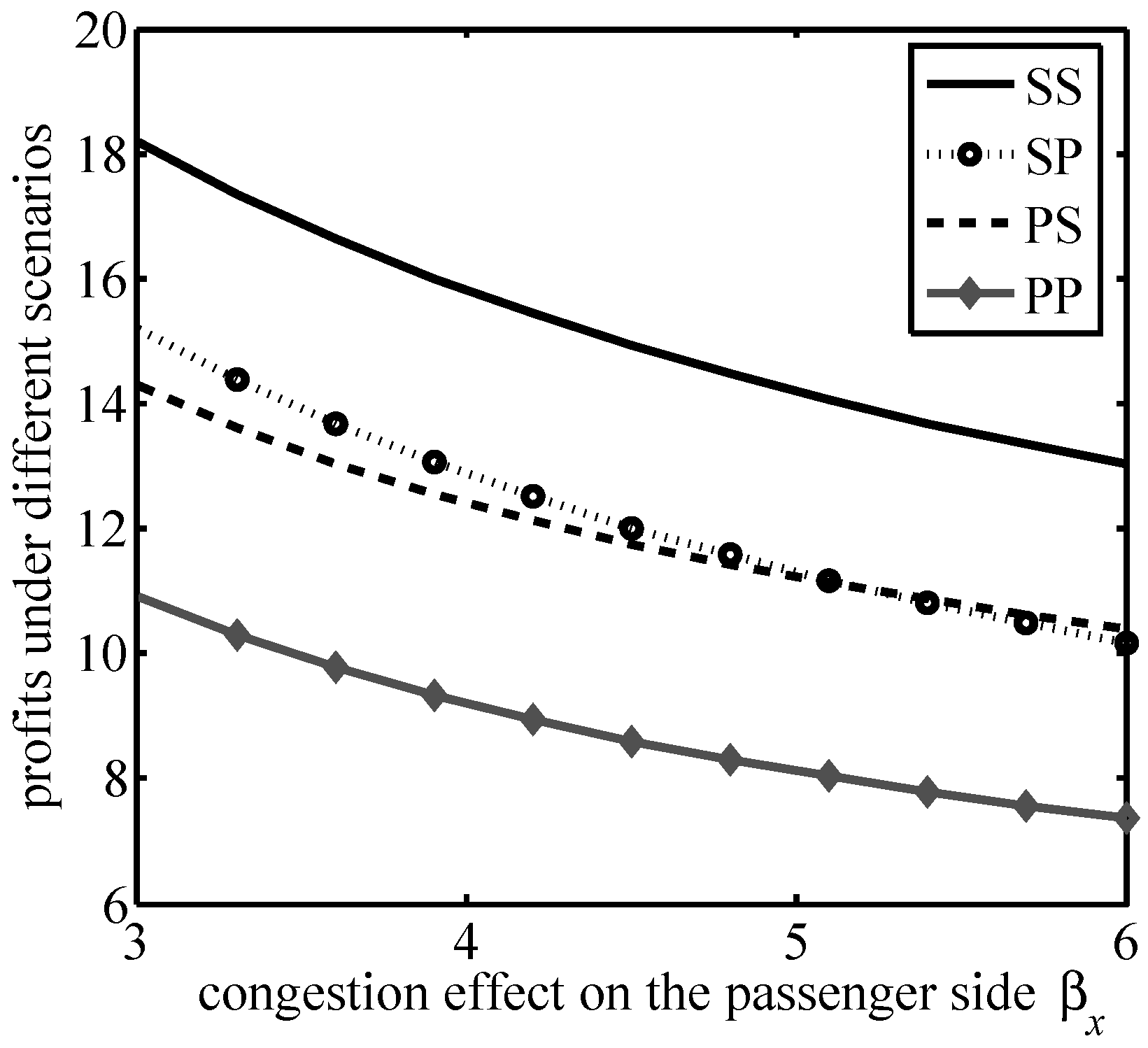
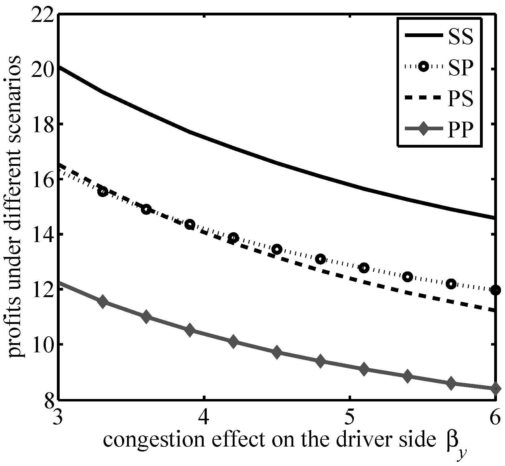
Let $V=10$, ${\alpha }_x=1.1$, ${\alpha }_y=1$, ${\beta }_x\in \left(3,6\right)$, ${\beta }_y=5$, $\delta =0.5$, which provides the variation of the platform profit with ${\beta }_x$, as shown in Figure 1. 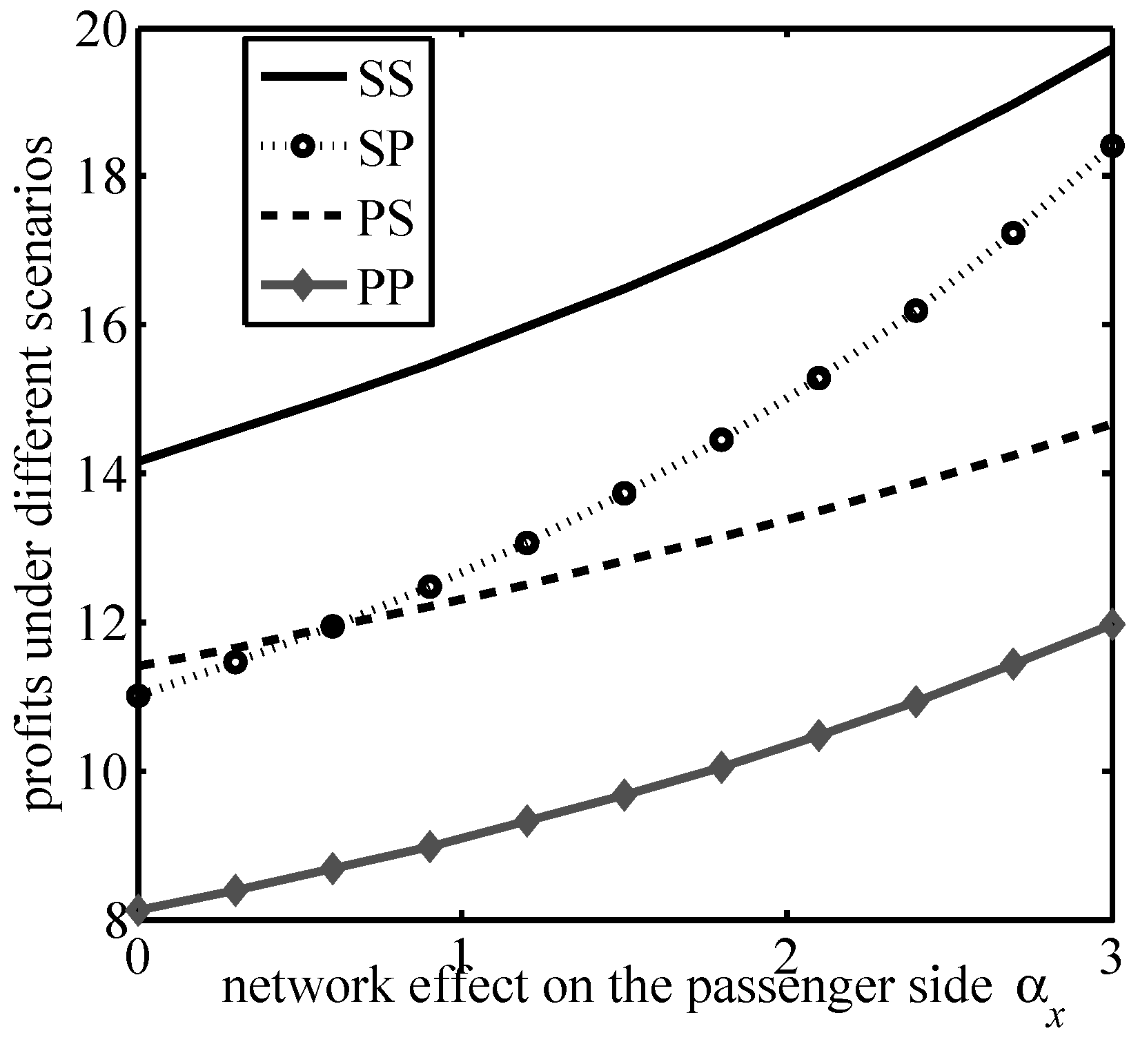Let $V=10$, ${\alpha }_x=1.1$, ${\alpha }_y=1$, ${\beta }_x=4$, ${\beta }_y\in \left(3,6\right)$, $\delta =0.5$, which yields the variation of the platform profit with ${\beta }_y$, as shown in Figure 2. 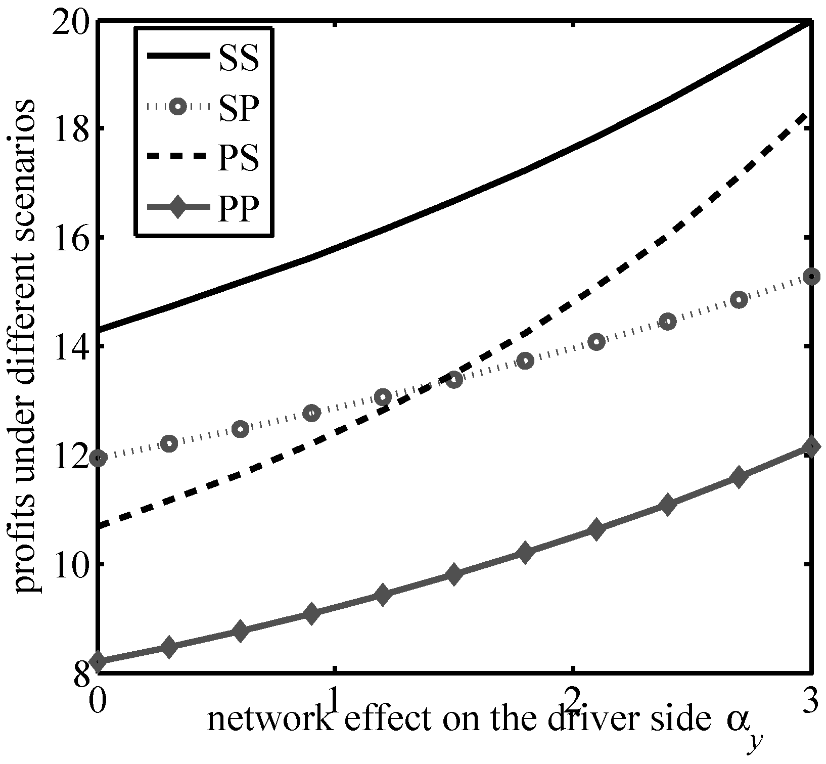Let $V=10$, ${\alpha }_x\in \left(0,3\right)$, ${\alpha }_y=1$, ${\beta }_x=4$, ${\beta }_y=5$, $\delta =0.5$; the variation of the platform profit with ${\alpha }_x$ can be obtained as shown in Figure 3. Let $V=10$, ${\alpha }_x=1.1$, ${\alpha }_y\in \left(0,3\right)$, ${\beta }_x=4$, ${\beta }_y=5$, $\delta =0.5$, which provides the variation of the platform profit, as shown in Figure 4.

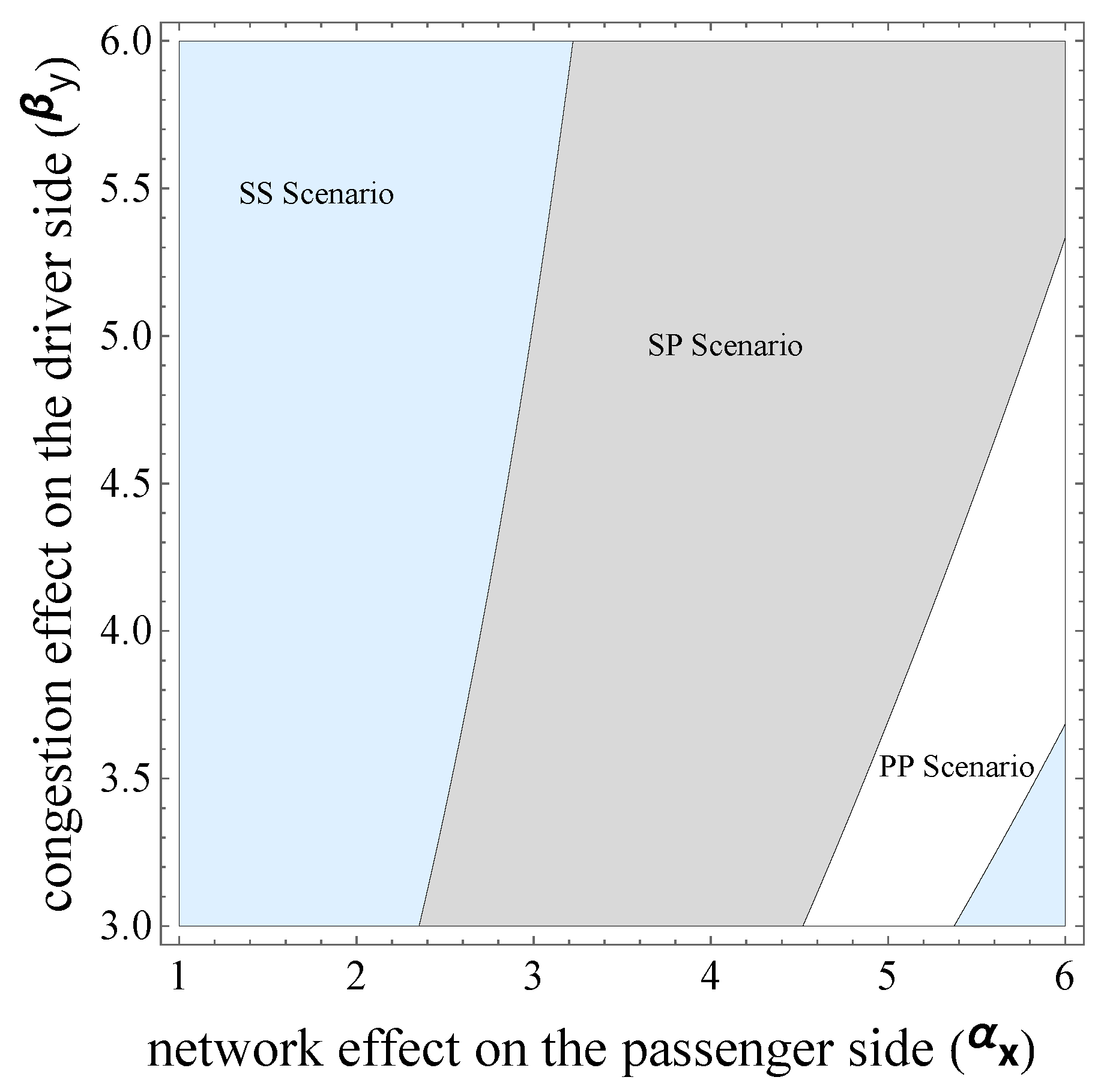
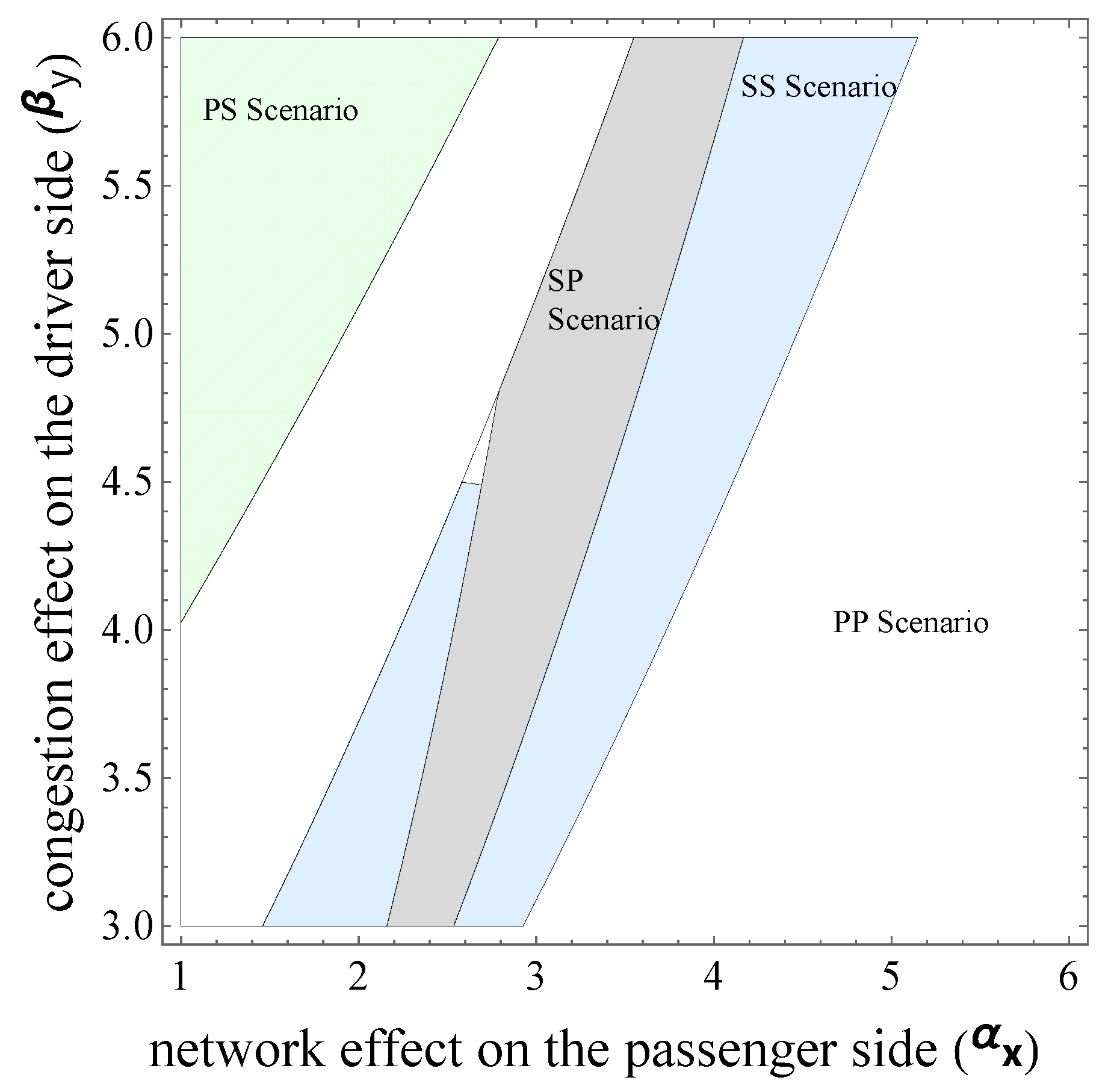
Let $V=15$, ${\beta }_x=2.7$, ${\alpha }_y=1.6$, $\delta =0.47$, ${\beta }_y\in \left(3,6\right)$, ${\alpha }_x\in \left(1,6\right)$, which provides the comparison of profits in different scenarios, as shown in Figure 5. Let $V=15$, ${\beta }_x=1.8$, ${\alpha }_y=4.5$, $\delta =0.47$, ${\beta }_y\in \left(3,6\right)$, ${\alpha }_x\in \left(1,6\right)$, which provides the comparison of profits in different scenarios, as shown in Figure 6.

From Figure 1, Figure 2, Figure 3 and Figure 4, it can be verified that the ride-hailing platform’s profits in all four scenarios decrease with the increase in the congestion effect on both sides, while profits increase in all four scenarios with the increase in the cross-group network effect on both the passenger and driver sides. These results are consistent with those in Propositions 1–4, with an increase in the cross-group network effect being beneficial to the platform’s profitability and the congestion effect on both sides is detrimental to the platform; thus, the platform needs to take measures to alleviate congestion on both sides in order to increase profits.

Figure 5 and Figure 6 compare the profits of the ride-hailing platform in the four scenarios. First, for the overall trend, Figure 5 and Figure 6 show that the platform is able to make the highest profit in each scenario. Second, the results of the profit comparison between the four scenarios depend on the cross-group network effects and congestion effects on both the passenger and driver sides. When the cross-group network effects on both sides are small, the SS scenario makes the highest profit. As the cross-group network effect on the passenger side increases, the SP scenario makes the highest profit, followed by the PP scenario.

When the cross-group network effects on both sides are large, the PP scenario makes the highest profit. As the congestion effect on the driver’s side increases, the SS scenario makes the highest profit, followed by the SP scenario. Finally, when the inter-group network effect on the passenger side is small and the inter-group network effect on the driver side is large, the SS scenario makes the highest profit. As the congestion effect on the driver side increases, the PP scenario makes the highest profit, followed by the PS scenario.

6. Conclusions and Managerial Implications

In this paper, we have constructed a game-theoretic model to analyze the pricing of ride-hailing platforms (e.g., Didi Rider, Lyft, and Uber) under the influence of the cross-group network effect and the congestion effect while considering the differences in price and hassle cost perceptions between passengers and drivers, with the following findings. (1) when both passengers and drivers are sensitive to hassle costs, if the cross-group network effect on the passenger side is higher than that on the driver side, the platform’s pricing on both sides increases with the strength of the congestion effect; otherwise, the prices on both sides of the platform decrease with the increase in the congestion effect. (2) When passengers are sensitive to hassle costs and drivers are sensitive to price, if the ratio for passengers’ and drivers’ different perceptions of price and hassle cost is greater than a certain threshold, the platform’s pricing on the passenger side should increase with the increase in the congestion effect, while the platform’s pricing on the driver side should decrease with the increase in the congestion effect; otherwise, the platform’s pricing on the passenger side should decrease with the increase in the congestion effect, while the platform’s pricing on the driver side should increase with the increase in the congestion effect. (3) When passengers are sensitive to price and drivers are sensitive to hassle costs, if the ratio for passengers’ and drivers’ different perceptions of price and hassle cost is greater than a certain threshold, then the platform’s pricing on the passenger side should decrease with the increase in the congestion effect, while the platform’s pricing on the driver side should increase with the increase in the congestion effect; otherwise, the platform’s pricing on the passenger side should increase with the increase in the congestion effect, while the platform’s pricing on the driver side should decrease with the increase in the congestion effect. (4) When both passengers and drivers are price sensitive, if the cross-group network effect on the passenger side is larger than that on the driver side, the platform should decrease its pricing on both sides with the increase in the congestion effect; otherwise, if the cross-group network effect on the passenger side is less than that on the driver side, the platform should increase its pricing on both sides with the increase in the congestion effect. (5) The platform is able to generate the highest profit in each scenario; the results of our profit comparison between the four scenarios shows that it depends on the cross-group network effects and the congestion effects on both the passenger and driver sides.

A number of managerial insights can be derived from this paper. (1) With the expansion of user scale, ride-hailing platforms should pay more attention to the impact of the cross-group network effect and the congestion effect on bilateral matching, and should reasonably adjust bilateral pricing according to the variability of bilateral users’ perceptions of hassle costs and prices to improve matching efficiency and increase platform profits. (2) Ride-hailing platforms should focus on the impact of the congestion effect in order to avoid causing loss of user scale and a reduction in platform revenue. The impact of both the cross-group network effect and the congestion effect should be considered for dynamic pricing on both sides. The findings of this paper can provide lessons for the bilateral pricing and operational management of ride-hailing platforms.

Future research could further explore the following aspects. First, in this paper we have only considered the monopoly scenario, and have not yet considered the bilateral matching decisions of ride-hailing platforms in scenarios with competition. Second, in this project we have assumed that ride-hailing platforms charge a one-off fee to successfully matched passengers and drivers, and have not considered the proportional fee scenario. Third, in this paper we have only considered pricing in one period; future research could consider dynamic pricing for both passengers and drivers.