


1. Introduction
Snow avalanches are a major threat in mountainous regions throughout the world. Advancing the current knowledge on the flow dynamics and particularly the resulting mobility and destructiveness of avalanches, is key to enhance existing mitigation strategies and adapt to expected future challenges resulting from climate change (Lazar and Williams, Reference Lazar and Williams2008; Castebrunet and others, Reference Castebrunet, Eckert, Giraud, Durand and Morin2014; Faug and others, Reference Faug, Turnbull and Gauer2018; Köhler and others, Reference Köhler2018). Furthermore it is necessary to deepen the understanding of transport phenomena of debris or victims in avalanches with respect to possible trajectories, expected accelerations, loads or resulting burial depths. This understanding allows to further investigate the functional principle of inflatable avalanche airbag systems, which rely on segregation processes (Gray and Ancey, Reference Gray and Ancey2015), or to expedite the development of future rescue systems. The flow dynamics of snow masses depend on a multitude of factors that are complicated to assess, due to the difficulty of performing repeatable, reliable and comparable experiments. To enhance the current avalanche understanding, computational and experimental efforts are necessary on all scales. Computational modelling approaches or experimental, laboratory setups have recently allowed to investigate detailed effects from small to large scales (Thibert and others, Reference Steinkogler, Gaume, Löwe, Sovilla and Lehning2015; Fischer and others, Reference Fischer, Kaitna, Heil and Reiweger2018; Gaume and others, Reference Gaume, van Herwijnen, Gast, Teran and Jiang2019). Field experiments mainly concentrate on the continuum behaviour of the avalanche flow (Faug and others, Reference Faug, Turnbull and Gauer2018), while obtaining information at the particle level in field observations remains particularly challenging. The destructive nature of an avalanche requires durable measurement equipment that is installed prior to the event, inside the flow path and can interact with the flow. Conversely, close-range sensing techniques like video, radar or laser scanning, are employed to remotely record data from a safe location (e. g. the valley floor, a counter slope or an aerial platform) (Eckerstorfer and others, Reference Eckerstorfer, Bühler, Frauenfelder and Malnes2016). Full-scale avalanche experiments are mostly performed at well-confined test sites. Notably, important test sites are Valleé de la Sionne in Switzerland (Sovilla and others, Reference Sovilla2013), Ryggfonn in Norway (Gauer and others, Reference Gauer2006) and Col de Lautaret in France (Thibert and others, Reference Thibert2015). However, these sites each have specific limitations that hinder frequent avalanche experiments (i.e. size, remote location or difficult access Barbolini and Issler, Reference Barbolini and Issler2006). A majority of the avalanches occurring at Valleé de la Sionne and Ryggfonn spontaneously release, thus mostly escaping scientific scrutiny. Besides a wide range of other instruments, the Swiss test site is equipped with a 20 m high steel pylon that houses pressure plates, optical velocity sensors, infrared temperature probes and density sensors at different heights to record a vertical flow profile. Similar structures with different kind of pressure sensors have been installed at the Ryggfonn and Col de Lautaret sites. While such data provide a very detailed vertical flow profile at a single location, spatially explicit velocity data of an avalanche event can only be remotely sensed. In recent years, radar technology has delivered valuable contributions in the characterisation and measurement of avalanches (Köhler and others, Reference Köhler, McElwaine and Sovilla2018). Two long-range radar types are usually applied in avalanche measurements: A Doppler radar records the velocity distribution of all approaching lumps of snow in a range-gated volume over time using the Doppler effect (Gauer and others, Reference Gauer2007). A range gate is typically only 25 m long and is sampled at several pulses per second. However, a much finer resolution can be achieved with a frequency modulated continuous wave (FMCW) radar. FMCW radar can achieve sub-metre resolution at around 100 Hz pulse repetition rate. Changes between consecutive pulses can be enhanced during post processing, yielding a moving target indication, which is typically displayed in a range-time diagram (Köhler and others, Reference Köhler, McElwaine and Sovilla2018). Both radar systems are valuable tools to track an avalanche's evolution along the path, and identify flow regimes and changes thereof (Faug and others, Reference Faug, Turnbull and Gauer2018). An experimental measurement technique that has previously been applied in snow chute experiments (Vilajosana and others, Reference Vilajosana, Llosa, Schaefer, Surinach and Vilajosana2011) and recently gained attention in full scale rockfall applications (Volkwein and Klette, Reference Volkwein and Klette2014; Caviezel and others, Reference Caviezel2021; Noël and others, Reference Noël2022) are in flow sensors, which travel with the flow and record corresponding motion data. Thus, instead of observing the avalanche flow from an Eulerian point of view where the flow passes a specific location over time, inflow sensors represent a Lagrangian way of following the flow as an immersed particle, thus assessing the flow condition along a flow trajectory. A predecessor of inflow sensors are the sensor and experiments of Fischer and Rammer (Reference Fischer and Rammer2010); Winkler and others (Reference Winkler2018), that deployed a ball equipped with a global navigation satellite system (GNSS) and inertial measurement unit (IMU) in an avalanche in 2013. However, their system never got fully developed and remained a single prototype lacking reliable tracking of its location in the avalanche, because of the used hardware, that was designed for drone operations. Similar ideas have been successfully employed in rock fall studies (Caviezel and others, Reference Caviezel2019). Their focus lies on the characterisation of discrete impact forces, therefore the sensors where only equipped with an IMU. They were also able to reproduce the rockfall trajectories with videogrammetry, which is not suitable for avalanche experiments.
We present a new in-flow sensor system that resembles the motion of snow particles in an avalanche, e.g. the size and density are in the same order of magnitude as expected from the granulometry of an avalanche composition (Bartelt and McArdell, Reference Bartelt and McArdell2009). These AvaNodes are equipped with two different tracking technologies, IMU and global navigation satellite system (GNSS), as well as an infrared thermometer.
Thus, the AvaNodes deliver independent data on particle movement of rather dense snow granules in an avalanche. The presented experiments were all performed at the newly established test site Nordkette, directly above Innsbruck (Austria), which is easily accessible and provides frequent opportunities for avalanche experiments due to the regular avalanche control work being carried out there for ski resort safety. However, the avalanche type is limited to medium-sized, cold-dry dense flow avalanches.
In this paper we focus on the potential of GNSS tracking in avalanche experiments, supported by IMU and radar measurements, and discuss how accurate the datasets are under the influence of covering snow layers. The derived particle velocity data allows dividing the avalanche flow into the main three states of acceleration, steady state and deceleration. During these three stages of temporal velocity development, the accelerometer and gyroscope data indicate different flow conditions.
Following this introduction, a methods section 2 covers the description of the Nordkette test site in Sec. 2.1, the AvaNode inflow sensors in Sec. 2.2 and a summary of the avalanche experiments in Sec. 2.6, as well as the data preparation and processing. The results are given in Sec. 3 and a discussion thereof follows in Sec. 4, with a final conclusion in Sec. 5 and an outlook in Sec. 6.
2. Methods
2.1 Avalanche test site Nordkette
The avalanche test site is located at the Nordkette ski resort, which is situated above Innsbruck in Western Austria. The site is accessible year-round via cable way from the city centre in 40 min, and is a popular tourist destination. The mountain crest above the site lies at about 2300 m a.s.l. and splits into several avalanche paths, fitted with different remote avalanche control systems (Fig. 1). The terrain consists of several steep couloirs with slope angles larger than 35 °, separated by rock faces.

Figure 1. Panels a and b give an overview of the Nordkette avalanche test site with the Seilbahnrinne avalanche path in blue. The release area (light blue) is next to the Hafelekar station. Green lines indicate the deflection dam at 1,900 m a.s.l. and the catching dam at 1,800 m a.s.l. The deposition zone (light pink) starts at around 2,050 m a.s.l. and typically ends near the dam at 1,800 m a.s.l. The avalanche thalweg (blue line) follows the main trajectory in flow direction. All snow and avalanche observations are carried out from Seegrube, including snow pit, camera and radar (radar field of view shown in light grey). Automatic weather stations are located west of Seegrube.
Large amounts of snowfall are common when a Nordstau weather situation brings precipitation from northerly to north-westerly directions. Single day new snow rates of one metre are frequent and multi day storm events can bring considerable amounts of new snow. The yearly solid precipitation sum is 10 m on average in the winter months, with a minimum and maximum of 5 m and 15 m, respectively (Avalanche Commission Innsbruck, 1966–1992). Continuous avalanche control is carried out throughout the winter season after more than 30 cm of fresh or wind drifted snow in the release areas, to ensure the safety of the underlying ski resort and infrastructure. This framework was used to establish continuous snow measurements and avalanche experiments throughout the winter seasons 2020/21 to 2022/23 at this site.
The main avalanche path featured in this study is the Seilbahnrinne (47$^\circ$ 18’44”N, 11$^\circ$
 22’60”E, 2,269 m a.s.l.), situated directly below the cable way running up to the ridge. The inflow sensor system AvaNode is thrown in the release area, close to the control station of the blasting cable way, before avalanche blasting. The release area is confined by a steep rock face to the west and a ridge to the east (size approx. 2,750 m2, exposition S to SW, average slope angle 46 °).
The Seilbahnrinne joins the Juliusrinne avalanche path at 2150 m a.s.l., and continues relatively confined until 2000 m a.s.l. Below, the path runs onto a wide scree slope where the slope angle decreases to around 30 °. The deposition zone ends at an artificial avalanche dam at 1800 m a.s.l., resulting in a potential total drop height of 450 m and a slope parallel length of 845 m.
The release thickness typically varies between 0.3 m and 1 m and is predominantly governed by the amount of new snow that accumulates in the release area, since ongoing avalanche control throughout the season continuously removes additional snow. In relation to the release area, this results in a volume of 825 to 2750 m3, which corresponds to an avalanche size 2 or medium sized avalanche, according to the European Avalanche Warning Service (EAWS) classification. Despite the small release volumes, the avalanches typically grow considerably due to entrainment along the path and usually reach the Seegrube and the deflection dam there at 1900 m a.s.l. In case of large precipitation events, followed by release depths beyond 1 m, avalanches may reach the dam at the end of the avalanche path.
The test site has been equipped with three automated weather stations for many years. Two stations next to the Seegrube are equipped with precipitation and snow height sensors; one station at the ridge is measuring wind speed. Furthermore, a manual snow stake is sampled every morning and a snow profile is recorded on each avalanche control day, focussing on the new snow temperature and density.
The Seilbahnrinne avalanches are observed with three separate cameras. One camera focuses on the release area and yields additional information about the starting point of the inflow sensors. The two other cameras are pointed at the avalanche path, one from the top and one from the bottom, to observe movement and deposition of the avalanche.
During the winter 2020/21 a mobile Doppler avalanche radar (Rammer and others, Reference Rammer, Kern, Gruber and Tiefenbacher2007; Fischer and others, Reference Fischer, Fromm, Gauer and Sovilla2014) was set up and avalanche velocity measurements manually recorded from the avalanche path. Since the winter 2021/22, a fixed FMCW radar mGEODAR installation continuously monitors the avalanches at the test site (Köhler and others, Reference Köhler2020). Unfortunately, both radar devices disturb each other and cannot be run simultaneously on the same avalanche path.
2.2 Inflow sensor system - AvaNode
The AvaNode is a newly developed system for motion tracking, capable of measuring accelerations and angular velocities via an IMU. In addition, a GNSS module is integrated, which measures longitude, latitude, altitude, Doppler velocities and world time besides other data. The AvaNode has the shape of a concave cube, in order to prevent rolling and sliding on the snow surface. The shape of the housing and interior hardware cube can be seen in Fig. 2. The housing can be replaced at any time when damaged, to preserve the used hardware and minimise costs. Due to the inherent avalanche danger during the experiments, the AvaNode is dropped or thrown into the release area from above, considering respective safety measures. The density of the AvaNode is 415 kgm−3, for Nodes C01, C03, C09 and C10. The actual expected density for snow particles in avalanches is 300–500 kgm−3 (Schaer and Issler, Reference Schaer and Issler2001; Thibert and others, Reference Steinkogler, Gaume, Löwe, Sovilla and Lehning2015). Due to hardware and material properties it has so far not been possible to make a lighter version. The geometry is also determined by the space requirements for the hardware, resulting in a cube with a side length of 16 cm. In addition to the reference AvaNode, various variants were produced in order to map as many different particle properties as possible. So far three variants are in operation, one type with a higher density of 688 kgm−3 (AvaNodes C06 and C07), a second with a spherical shape and a third with an eight times higher volume. During the course of the measurement seasons, AvaNode generations I and II were developed. The second generation featured increased and more stable battery life, upgraded GNSS measurements (included Doppler velocities) and a more reliable hardware setup for this harsh environment.
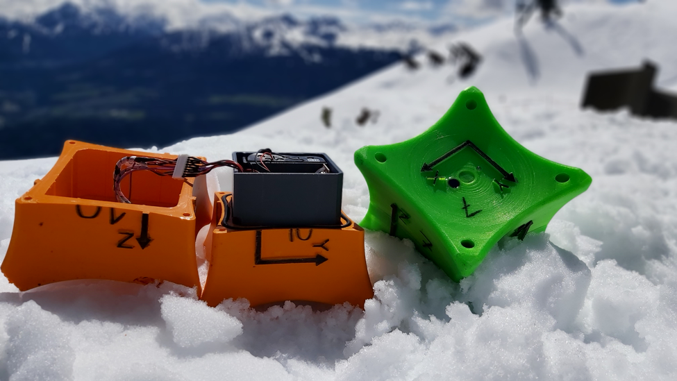
Figure 2. The figure displays two generation II AvaNodes employed in the experiments, namely AvaNode C10 (orange) and AvaNode C07 (green). AvaNode C10 has a density of ρ = 415 kgm−3, while C07 represents a density variation with a density of ρ = 688 kgm−3. It is important to note that the density is solely determined by the housing of the AvaNode, while the internal hardware remains consistent for both devices.
2.3 GNSS measurements
The utilised GNSS sensor module is based on a ublox CAM-M8Q chip, which is a standard precision GNSS chip. The module has a omnidirectional antenna to give best reception in the moving and strongly rotational flow of an avalanche. The chip determines the position data in a global coordinate system as well as a direct measurement of the Doppler velocity. The manufacturer data sheet and manual (u-blox, 2022) provide the following specs: Horizontal position accuracy (σ p,h) and Doppler velocity accuracy (σ v,d) are 2.5 m and 0.05 ms−1, respectively; operational limits for altitude, velocity and acceleration are 12,000 m, 310 ms−1 and 40 ms−2, respectively. No information is available for the vertical position (altitude) accuracy σ p,v.
The module is set up to simultaneously receive the signals from GPS (L1C/A at 1,575.42 MHz) and GLONASS (L1OF at 1602 MHz +k*562.5 kHz for each channel k = −7, …, 6). This increases the number of available satellites in confined terrain of channelled avalanche paths, where less than half of the sky is visible. Furthermore, using both GNSS constellations gives the most accurate position data and reduces the cold start time, but limits the navigation update rate to 10 Hz. U-blox receivers make use of dynamic platform models to adjust the navigation engine to the expected environment. The settings improve the receiver's interpretation of the measurements for a more accurate position output. For the presented measurements the dynamic platform model portable is used, which is suitable for applications like portable devices or in this case avalanche measurements. Before the input data gets passed to the navigation engine, it has to pass the navigation input filters. Their FixMode parameter is by default set to Auto2D/3D, which means that the receiver calculates a 3D position fix if possible, but reverts to a 2D position if necessary. Since the altitude information of the AvaNode can later also be extracted from a digital elevation model, this parameter setting is used. In this paper we used only altitude values derived by the GNSS module. All other navigation input and output filters are not set or were left at default values.
2.3.1 GNSS and snow
The experiments by Schleppe and Lachapelle (Reference Schleppe and Lachapelle2006) showed that it is possible to track GNSS signals under an avalanche deposit, but accuracy decreases depending on the thickness of the snow cover and its properties. One major factor that influences the L-Band signal and therefore the accuracy, is the liquid water content. In dry snow, with a density of 300 kgm−3, the GNSS signal, with ~1.5 GHz, gets attenuated by 4.3 dB per 400 m, this increases to 4.3 dB per 3 m when the snow has a liquid water content of 1$\%$ (Schleppe and Lachapelle, Reference Schleppe and Lachapelle2006). Koch and others (Reference Koch2019) use this feature to determine the liquid water content of the snow cover by comparing simultaneously acquired attenuated GNSS signals received under the snow cover and reference signals measured above snow. Furthermore, they were able to determine the snow water equivalent and the height of the snow cover. In order to be able to precisely delimit the performance of our low-cost GNSS modules under the influence of snow cover, experiments similar to those of Schleppe and Lachapelle (Reference Schleppe and Lachapelle2006) were planned and carried out. Three AvaNodes were buried at different snow depths, i.e. 0.5/1/1.5 m, which represent typical burial depths. An additional reference AvaNode was set onto the snow surface. The location of each AvaNode was surveyed to determine the AvaNode position and velocity accuracy. A more detailed description and evaluation follows in Sec. 3.1.
2.3.2 GNSS time synchronisation and normalisation
Time is delivered in universal coordinated time (UTC), with date and time. When performing experiments with several AvaNodes, one gets independent datasets for every AvaNode. To achieve comparability, temporal synchronisation of the datasets is necessary. For this the GNSS UTC is used. To compare datasets from different experiments, a normalised time scale t norm is introduced, which ranges from 0 to 1, where 0 or t min indicates the start of the movement and 1 or t max the end for every measurement. The duration of the movement is described by Δt = t max − t min, while the normalised time t norm provides an relative overview of the general movement from release (t norm = 0) to deposition (t norm = 1).

2.3.3 GNSS positions and trajectory
The position and global timestamp during the avalanche experiment are obtained by the GNSS module. The position is delivered in the real worlds coordinates longitude (x), latitude (y) and elevation (z) with respect to the WGS84 coordinate system. We define the projected and three dimensional travel length (s xy and s xyz) along each individual particle trajectory. The corresponding total projected and 3D trajectory or runout length (Δs xy, Δs xyz) is accordingly defined from start (t min) to the end (t max) of the movement.


The overall altitude difference is given by Eqn. (4). Combined with the projected travel length s xy, it is possible to calculate the runout angle α (Heim, Reference Heim1932; Körner, Reference Körner1980; Lied and Bakkehøi, Reference Lied and Bakkehøi1980; Bakkehøi and others, Reference Bakkehøi, Domaas and Lied1983) as given in Eqn. (2.4).


2.3.4 GNSS velocity
The position velocity v p is obtained from the GNSS module by calculating the time derivative of the 3D trajectory length s xyz. The derived velocities v p are gently smoothed with a moving average of kernel size n = 2 or 2 time steps. With a frequency of 10 Hz this results in a smoothing over 0.2 sec. In this paper, we refer to the calculated velocities v p with their origin in the position data as the position velocities. Clearly, the accuracy of v p is linked to the accuracy of the horizontal σ p,h and vertical position data σ p,v. The GNSS module allows to directly measure velocities via the Doppler shift in the GNSS frequency between the satellite and AvaNode motion. The processing is done in the GNSS chip and the Doppler velocities are delivered in the same coordinate system as position with the axes East, North, Down as v east, v north and v down. The absolute Doppler velocity v d is calculated by euclidean norm. The setting to write out the Doppler velocities is not default and has only been enabled for measurements beginning with season 2021/22, e.g. in the AvaNode generation II. Compared to any derived velocity from position data, v d is much more accurate and reliable in the order of σ v,d, however, for consistency they are also gently smoothed with a moving average of kernel size n = 2. The Doppler velocities of the AvaNodes v d are referred to as Doppler velocity in this paper.
2.3.5 GNSS acceleration
When the GNSS velocities are derived over time, it is possible to calculate the corresponding accelerations, i.e. the effective acceleration in the direction of movement, along the particle trajectory. To calculate the accelerations, the velocities were smoothed using a kernel size of n = 40 or 40 time steps. A detailed description and sensitivity analysis on the kernel size is delivered in Appendix A in Sec. A. The temporal resolution is defined by the frequency of the GNSS module with 10 Hz, therefore a kernel size of n = 40 results in a smoothing over 4 s. Accelerations derived from position velocity v p are referred to as position acceleration or a p, analogously accelerations derived from Doppler velocity v d are referred to as Doppler accelerations a d. These accelerations give an overview, whether the AvaNode is accelerating or decelerating, which equals to positive or negative accelerations.
2.4 IMU measurements
The AvaNodes contain an IMU type MPU9250, which is capable of measuring spatial translational accelerations, angular velocities, and magnetic flux densities with measuring ranges of ±16 g, $\pm 2000^\circ$ s−1, and ±4800 μT, respectively. The accelerations and angular velocities are stored on an SD card with a sampling frequency of 400Hz. Thus, the IMU provides detailed information on the dynamics of the AvaNode. Measured accelerations add a redundancy to translational motion information besides GNSS positions and velocities, which may be combined in future sensor fusion. In contrast to translational motion, orientation of the AvaNode can only be determined utilising the angular velocity and magnetic flux density measurements of the IMU. Local orientation is computed from measured angular velocities. Orientation with respect to the earth frame can be derived via a Gram-Schmidt projection utilising standstill data from the accelerometer and magnetometer (Neurauter and others, Reference Neurauter, Hergel and Gerstmayr2021). Due to drifting accelerometer data, special motion reconstruction algorithms are applied that require specific IMU data processing and a corresponding sensor calibration (Neurauter and Gerstmayr, Reference Neurauter and Gerstmayr2022).
2.4.1 IMU acceleration and rotation rates
The collected accelerations and rotation rates (angular velocities) from avalanche experiments are examined with respect to their euclidean norm. Furthermore, this data delivers precise indications if the object is moving or not, due to high sampling frequency and access to raw (unfiltered) data. This is used to determine start and end time (t min, as well as t max) of the sensor movement, which are then used in the further calculations. When an IMU is at rest the resulting euclidean norm will deviate from the gravitational acceleration g = 9.81 ms −2, due to the measuring principle of an IMU. The deviation between the magnitude of the measured accelerations at rest before the movement and g is given as Δg. This deviation was used to homogenise the accelerations towards g in rest position, so that they are comparable afterwards. The homogenisation has to be done by scaling the dataset, with the scaling factor f, calculated by:

The whole dataset from this measurement is multiplied with this factor. This does not include an in depth calibration which would consider an sensor offset and corresponding time drift (Neurauter and Gerstmayr, Reference Neurauter and Gerstmayr2022). The accelerations and rotation rates are not smoothed at all, because when heavy impulsive impacts occur during the experiment, it should be noticeable in the measurement data.
2.5 Radar measurements
The avalanche experiments are accompanied by an avalanche radar in all measurement seasons. Radar is independent of the visibility conditions and gives a good overview of the type and size of the avalanche. The radar is positioned at the Seegrube station and observes the avalanches moving towards its location, see Fig. 1. Due to a slightly oblique angle between main avalanche flow direction and the radar line-of-sight, any velocity estimations from the radar must be compensated for by the angle between the line-of-sight and the flow direction (Fischer and others, Reference Fischer, Fromm, Gauer and Sovilla2014). For the used setup, a maximum angular deviation of 15 ° was determined, resulting in a correction factor of +3.5$\%$ for the ground-parallel velocity. Both radars use a frequency of 10 GHz, which equals 3 cm wavelength and roughly resembles the size of relevant reflectors. Thus, mostly the dense flowing layers in the avalanche are imaged (Gubler and Hiller, Reference Gubler and Hiller1984).
In season 2020/21, a commercially available mobile pulse-Doppler radar from IBTP Koschuch was used (Koschuch, Reference Koschuch2018). Such a pulse-Doppler radar resolves a full velocity spectrum of the avalanche flow for each recorded pulse and in each range gate (Gauer and others, Reference Gauer2007). However, the achievable pulse rate is in the range of 1 Hz to 10 Hz, and the range resolution (range gate width) is typically 15 m to 30 m. Since the this radar was not permanently installed, the antenna orientation differed between each experiment and some data were lost due to orientation error caused by poor visibility conditions.
In season 2021/22, the mGEODAR radar was permanently installed at the Seegrube station. This is a frequency-modulated continuous-wave (FMCW) type radar and custom-made for research purposes (Köhler and others, Reference Köhler2020), based on the Swiss GEODAR radar (Ash and others, Reference Ash2014). The radar has a high pulse repetition rate of 100 Hz and a range resolution of 0.3 m. However, a direct velocity estimation is not yet achievable for the distributed target of an avalanche. The frontal approach velocity is indirectly estimated by tracking the clear front line in a range-time diagram (Köhler and others, Reference Köhler, McElwaine and Sovilla2018). Again, since the radar data enables an overview of where the AvaNode is located in the avalanche body, we reduced the velocity estimation only to the maximal frontal approach velocity, i.e. to the point where the front line is steepest.
The radar and AvaNode data are timed by separate clocks. The pulse-Doppler radar has a real-time clock that might be subject to drift. The mGEODAR radar has a synchronised time from the internet. Nevertheless, there are always synchronisation issues in the range of seconds. Here, we manually shift the radar time against the AvaNode time to match the first motion from the IMU data with the detected motion in the radar data. Since the velocity evolution starts with relatively low flow velocities in the first seconds, usually not more then 5 ms−1, an uncertainty in the shift of 1 sec to 2 sec equals a position uncertainty of 5 m to 10 m.
The supplementary radar measurements allow relating the AvaNode positions to total avalanche flow and particularly the actual location of the avalanche front. The radar resolves the line-of-sight distance or range, and the whole avalanche is laterally averaged. However, the Seilbahnrinne is a very confined avalanche path and the lacking lateral resolution of radar is considered not to be relevant here. Another limitation of both radars is the limited opening angle of the antenna of 8 ° horizontally, so that the avalanche flow is only tracked from the release area down to an elevation of 1,950 m a.s.l., which roughly corresponds to a range of 200 m. This is enough to capture the relevant portion of the avalanche to locate the AvaNodes, but no information can be inferred about the stopping of the avalanche front.
2.6 Static snow cover and dynamic avalanche experiments
2.6.1 Static snow cover experiments: set-up
To estimate the influence of the snow cover on the accuracy of the position, velocity and acceleration data, four AvaNodes were buried in the static snow cover on the 25 January 2022. Each AvaNode was buried at a different depth of 0.5 m, 1 m and 1.5 m, respectively, with a reference on top of the snow cover at 0 m. The experiment took place at Seegrube, so the conditions defined by the terrain and the visual portion of the sky are comparable to the situation during the avalanche experiments. A precise snow profile was not acquired, since during burying the AvaNodes, any snow layering was destroyed and the covering snow was homogenised. The snow cover at the time of the experiments was dry, with temperatures ranging from −1.1 to −4.9 °C and densities between 150 and 400 kgm−3. Clearly, this experiment covers only the situation for such particular snow cover situation. However, all avalanche experiments occurred with freshly fallen dry snow. The locations of each AvaNode were measured with a precise multi-band differential GNSS receiver (Emlid Reach RS2). The standard deviation of the horizontal and vertical position data from the RS2 was about 2–3 cm on that day. The duration of the experiment was about three hours and yielded more than 100,000 individual GNSS position samples. Fig. 3 summarises the results from the static GNSS experiment to assess the accuracy of position, velocity and acceleration at different burial depths.

Figure 3. This Figure shows the position, velocity and acceleration deviation, from left to right, dependent on the snow cover for the used GNSS module. The black dashed line indicates the horizontal position accuracy of 2.5 m and the Doppler velocity accuracy of 0.05 ms −1, as reported by the manufacturer. The reference velocity and acceleration was 0 ms −1 and 0 ms −2, since the AvaNodes were not moving during the experiment. The box plots show the median value, the boxes include 50 $\%$ of the dataset, reaching from 25 $\%$
 to 75 $\%$
 . The whiskers were defined with 1.5 times the interquartile range (IQR), values that did not fit in this range were classified as outliers and were not plotted.
2.6.2 Dynamic avalanche experiments: set-up
Whenever an avalanche experiment happened, the AvaNode sensors were powered on beforehand, such that the GNSS module adjusted to obtain position data and time synchronisation. Shortly before the avalanche blasting, the AvaNodes are simply thrown into the release area from the mountain ridge. The observation of the avalanches and control of the radar and camera equipment were performed from a safe observation position at the Seegrube station. The properties of the freshly fallen new snow, like temperature and density, were measured during the morning of the respective experiment day.
As soon as the avalanche control work was finished and the ski patrol granted access to the deposition area, the retrieval of the AvaNodes began. An eminent retrieval of the sensors was crucial, because the localisation transmitter should not run out of battery. Furthermore, the Seilbahnrinne ski run should be kept free of transmitting signals and passive reflectors that could interfere with a potential rescue operation. Usually, the AvaNodes are deposited roughly at the elevation of Seegrube and access was possible on foot or with touring equipment.
To ensure a quick retrieval of the AvaNodes, multiple, redundant recovery systems, like an avalanche cord for optical recovery (passive), a Pieps TX600 (active, additional frequency for common avalanche transceivers), Lambda4 Smilla (active) (Lambda4, 2023), and Recco rescue reflector (passive) were used.
Burial depths were recorded upon AvaNode recovery and were therefore confounded when no direct retrieval was possible or a potential secondary avalanches remobilised the AvaNode. Due to the avalanche control setup, Seilbahnrinne was usually the primary control point and consecutive releases potentially changed the AvaNodes's burial location and depth. In case the AvaNodes could not be retrieved on the day of experiment, additional new snow and avalanches from the next day potentially rendered any depth estimation useless.
While most AvaNodes could be recovered by optical search, the long-range localisation system Smilla proved to be advantageous, providing a direction and distance to up to four AvaNodes. For a close range search and precise localisation, a hand-held Recco transceiver helped to indicate the location of the passive Recco reflector in the field-of-view. Usually all sensors were recovered within less than a few hours after the experiments.
3. Results
Static experiments allowed to investigate the influence of the snow cover and particularly expected burial depths on GNSS (accuracy and precision) measurements, while the dynamic experiments facilitated the view into the avalanche at motion with respect to particle accelerations, rotation rates and velocities.
3.1 Static snow cover experiments
3.1.1 GNSS position
Fig. 3 shows the horizontal position deviation from the reference position measured with the RS2 receiver. The horizontal deviation is measured as distance from the reference point and can therefore only have positive values. The horizontal GNSS accuracy reported by ublox is 2.5 m for the ublox CAM-M8Q chip, and is defined by the circular error probable (CEP) over 24 h.
The CEP equals the radius of the circle around the reference, where 50$\%$ of the measurements are included (Diggelen, Reference Diggelen2007). This corresponds to the definition of the median of the box plots seen in Fig. 3. The median of the horizontal position deviation under snow cover was in the order of the GNSS accuracy for all burial depths. While the reference AvaNode on top of the snow cover had a lower accuracy with 2.7 m, at 0.5 m snow cover, it increased towards 2.3 m accuracy. Afterwards there was a slight decrease in the accuracy for burial depths of 1 and 1.5 m, towards 2.5 and 2.9 m, respectively.
3.1.2 GNSS velocities
Fig. 3 shows the recorded absolute velocities for the statically placed AvaNodes, i. e. the reference velocity was by definition 0 ms−1. The position velocities were calculated from the horizontal and vertical position data by time derivative (see Sec. 2.3) and no reference accuracy can be given. The Doppler velocities were recorded directly from the GNSS module with an accuracy of 0.05 ms−1, as reported in the data sheet.
The median Doppler velocity deviation was 0.047 ms−1 for the AvaNode on top, then decreased to 0.038 ms−1 for 0.5 m and 0.033 for 1 m, until it reached 0.047 again at 1.5 m, which corresponds to the median on top of the snow cover. For all burial depths the GNSS accuracy was lower then the one given by the manufacturer with 0.05 ms−1. The median position velocity deviation was 0.25 ms−1 for the AvaNode on top, then decreased to 0.2 ms−1 for 0.5 m and 0.17 ms−1 for 1 m, till it reached 0.25 ms−1 again, similar to the AvaNode on the top. Due to the fact that v p is calculated through the time derivative from the position data, it is not surprising that the median position velocity deviation is nearly one order of magnitude higher then the Doppler velocity median. However, the deviation for both velocity types showed a clear decrease for 0.5 m and 1 m burial depth compared to the reference measurement at the surface of the snow cover.
3.1.3 GNSS accelerations
Fig. 3 shows the calculated accelerations from the time derivative of the Doppler and position velocities (see Sec. 2.3). Again, zero acceleration is expected for the statically buried AvaNodes, thus any deviation comes solely from noisy GNSS data. On average, the position and Doppler accelerations were nearly zero for all burial depths. Obviously, the standard deviation was much higher for the position acceleration, with σ a,p = 2.18 ms−2, than for the Doppler acceleration with σ a,d = 0.28 ms−2. σ a,d is used in Sec. 3.2.4 for further analysis. Again, a slight decrease in the deviation is observed for 0.5 m and 1.0 m burial depth, with an increase to 1.5 m depth.
3.2 Dynamic avalanche experiments
In total, eight avalanche events with eleven recorded AvaNodes trajectories were performed. According to the international avalanche classification (avalanche atlas (UNESCO, 1981)), most observed avalanches classify as A2B1C1D2E2F4G1H1J4, corresponding to: slab avalanches (A2), with a sliding surface within the snow cover (B1) and dry snow (C1) in the zone of origin, channelled avalanches (D2), dominated by the dense, flowing part (E2) in the zone of transition and mostly fine (F4), dry (G1), clean (H1) deposits in the zone of deposition. All avalanches have been artificially triggered within avalanche control work (J4). Small classification variations appear concerning form of motion (some avalanches are mixed types with powder part, E7) and surface roughness of deposit (some avalanches have coarse deposit with rounded clods, F3).
3.2.1 Dynamic avalanche experiments: recorded events
Between March 2021 and March 2023 eight avalanches were successfully tracked with the AvaNode inflow sensors. The measurements in season 2020/21 were performed with AvaNode generation I and from season 2021/22 on with AvaNode generation II, that had a direct recording of the GNSS Doppler velocity information. Supplementary environmental measurements of the initial conditions (i. e. air temperature, snow depth, density and temperature) were recorded for each event. A short description of each avalanche is given below and Table 1 summarises the data from each AvaNode, while Table 2 summarizes each experiment or avalanche.
Table 1. Summary of the eleven AvaNode measurements in eight avalanches throughout season 2020/21, 2021/22 and 2022/23

The first block lists trajectory properties of each experiment. The second block summarises a first dynamic view on the experiments. A consistent colouring for each AvaNode is used for all visualisations in the following figures and given in the table row colour. The asterisk marks the sensors with higher density and v max, represented by the position velocity v p.
Table 2. Summary of the eight avalanche experiments throughout season 2020/21, 2021/22 and 2022/23

The first block lists radar and particle velocities, as well as burial depths of the AvaNodes. The second block summarises the deposition of the avalanches. The third block summarises the environmental data, that was collected during the experiment. The asterisk marks the sensors with higher density. The whole avalanche runout length and altitude difference are measured along the thalweg, which represents the avalanche trajectory along the main flow direction.
Avalanche 210315 was released on the first morning of a three day storm period. Strong wind during the night from northerly directions added to the loading of the release area, beside a snowfall of around 30–40 cm at air temperatures around $-6^\circ$ C. The wind calmed down during the experiment morning and together with increasing visibility the temperatures rose. One AvaNode (nr. C01) travelled with the avalanche and came to rest on top of the snow. Supplementary Doppler radar data are available for the avalanche. Due to a secondary avalanche from Juliusrinne (40 min later), the AvaNode was entrained again and kept rolling downwards after the original avalanche had stopped.
Avalanche 210316 was released on the second morning of the period described above. Strong northerly winds and a total of 70 cm new snow since the day before loaded the release area. No visibility, air temperatures around −6 $^\circ$ C and constant heavy snowfall (5 cmh−1) during the experiments. Two AvaNodes (nr. C01 & nr. C03) were successfully picked up by the triggered avalanche. The AvaNodes stopped roughly at the elevation of Seegrube, but the avalanche continued towards the catching dam at 1,800 m a.s.l. No supplementary radar measurements were available.
Avalanche 220123 was released after 23 cm of new snow. Air temperature was around $-6^\circ$ C and visibility was good. Avalanche data of one AvaNode (nr. C01) were successfully recorded. Unfortunately, no supplementary radar data was recorded due to Antenna misalignment.
Avalanche 220203 was released after 65–70 cm of new snow with a density of 130–150 kgm−3 even though the air temperature was was around $-6^\circ$ C. Visibility was poor. Avalanche data of one AvaNode (nr. C10) were be recorded. The AvaNode later got entrained by the Juliusrinne avalanche and the Node was carried a bit further. Supplementary mGEODAR radar data was recorded for both avalanches.
Avalanche 220222 was released after around 40 cm of new snow. Air temperature was around $-5^\circ$ C and visibility was poor. The weather was warm and sunny in the preceding weeks, such that the old snow cover was decreasing and stabilised. The avalanching snow and entrainment was therefore limited to only the freshly fallen new snow. Dilute parts of the avalanche reached the catching dam at 1,800 m a.s.l. Three AvaNodes (nr. C07, nr. C09 & nr. C10) were successfully picked up by the avalanche (nr. C07 being a high density Node). Therefore, particularly in combination with with the supplementary mGEODAR radar data, this avalanche event provided the most interesting dataset.
Avalanche 230203 was released after around 80 cm of new snow with a density varying between 60 and 140 kgm−3. The air temperature was around $-2.5^\circ$ C. The visibility was very good, and supplementary video footage is available. Unfortunately, no supplementary radar data is available. AvaNode C06, with high density, was successfully transported with the avalanche. The avalanche was one of the largest ones, which we were able to observe during our three years of experiments, and ended in the catching dam at 1800 m a.s.l.
Avalanche 230204 was released after around 45 cm of new snow with a high density of 200 kgm−3. The air temperature $-3.4\, ^\circ$ C. The visibility was poor and supplementary radar data is available. AvaNode C07, with high density, was successfully transported with the avalanche.
Avalanche 230315 was released after 37 cm of new snow with a density varying between 110 and 190 kgm−3. The air temperature was $-0.7\, ^\circ$ C. Visibility was very good and supplementary video and radar footage are available. AvaNode C10 was successfully transported with the avalanche. The avalanche was rather small and stopped between 1950 and 2000 m a.s.l.
3.2.2 GNSS positions and trajectories
The GNSS modules continuously tracked the position of the AvaNodes inside the avalanche flow in a global coordinate system. Fig. 4 summarises all eleven trajectories within the eight recorded avalanche events. Some quantities, like projected travel length s xy, travel length s xyz, altitude difference ΔZ, runout angle α and the position velocity v p, derived from the position data, are also given in Table 1 as an overview between all AvaNode measurements.

Figure 4. In the left panel, trajectories or GNSS positions of all avalanche experiments are displayed. The spacing of the isochronous sampled position data indicates the flow velocity, e.g. the herein called position velocity v p. The dot size is set to 5 m, which corresponds to the accuracy stated by the manufacturer. The hatched area represents the release zone. In the right panel the projected travel length Δs xy (t) and the altitude difference ΔZ (t) are shown.
Well defined are the start and end position, since the most probable position were estimated from an average over many position data points when the sensor was at rest. Since all AvaNodes were thrown into the release area from the same location, all start positions are very similar, i.e. within a distance of a 25 m radius. Given that each avalanche is slightly different, their end positions vary much more and spread in the deposition area within a distance of 180 m. Interestingly, all end positions are aligned in a 20 m lateral distance around the main flow path.
The horizontal travel length and altitude difference can be estimated directly from the GNSS data. The projected travel lengths varied between 168 m and 360 m, with an average of 206 m. The altitude differences ranged between 125 m and 257 m, with an average value of 203 m. Horizontal and vertical distances yielded the run-out or α-angle, that was with around 35±1 $^\circ$ and very similar for all AvaNode trajectories. Compared to the run-out angle, the slope angle at the end location, derived from a digital terrain model, was generally smaller and varied between 33 $^\circ$
 and 36 $^\circ$
 .
.
During the flowing phase, the position data points could not be averaged and the position deviation of around 2.5 m, found in the static burial experiments (Sec. 3.1), influence the accuracy. However, all trajectory lines in Fig. 4 are very smooth, indicating an internal navigation filter. Interestingly in this regard, an overshooting of the end position is sometimes observable, e. g. the end position of cyan, purple and yellow are uphill of the lowest recorded position. That indicates that the hardware depended Kalman-Filter suggests an ongoing movement in the particle trajectory direction, till enough measurements indicate that the module is now at rest at the end position. This is a known problem for the presented measurements and will be overcome in the future by using more reliable GNSS modules where one has access to the raw (unfiltered) datasets.
3.2.3 GNSS velocities
The GNSS velocity evolution over the normalised time scale from −0.1 to 1.1 t norm for all avalanches is shown in Fig. 5. For all measurements, Doppler velocities v d are available, position velocities v p were neglected due to their limited precision. The start and end of the movement (t norm = 0.0 and 1.0, respective) were manually estimated from the IMU acceleration and rotation data (see Sec. 2.3.2). However, the GNSS derived velocities do not directly rise at zero, nor indicate stand-still at t norm = 1.0. This is not a synchronisation mismatch as both sensors are sampled with the same clock, but must be due to the filtering in the GNSS module. This is particularly dominant after the avalanche comes to rest, and results in about 0.1 ⋅ t norm longer apparent motion when only considering GNSS data.

Figure 5. The top panel shows the GNSS position and Doppler velocities over the normalised time scale. Doppler velocities are plotted with a solid, position velocities are plotted dashed line. The coloured circles and triangles indicate the maximum velocity for every measurement, where the triangles indicate a measurement with a higher density AvaNode. The bottom panel shows the accelerations derived from the derivation of GNSS velocities. Again the accelerations derived from the position data are plotted with dashed lines. The black line represents the mean values of all GNSS Doppler accelerations. The grey areas indicate the three states for both panels: Light grey represents the acceleration state (0–30$\%$ ), medium grey the steady state flow (30–57$\%$
 ) and darker grey the deceleration state (57–100$\%$
 ).
).
Fig. 5 shows the avalanche motion on a single particle level, e. g. tracked and thus resembled by an AvaNode. Even though the plot contains data of eleven different AvaNodes in eight different avalanches, the velocity evolution is very similar on the normalised time scale. The maximum velocities were reached between 8.9 ms−1 and 17.1 ms−1 in the time range between 0.36 and 0.51 t norm. Note, that usually the maximum velocity is found at a time were the velocity is on a continuously high level, and thus, correlates well with the later defined second flow state of steady state.
A clear difference in precision of the velocity derived from position data v p and the directly measured Doppler velocities v d is clearly visible. Qualitatively, the variance of the position velocity (dashed lines) has more noise than any of the Doppler velocities (solid lines). From the static experiment in Sec. 3.1, this lower precision is clearly expected.
3.2.4 GNSS acceleration
As in Sec. 3.1, the accelerations were also considered for avalanche experiments and displayed in Fig. 5. The position accelerations were plotted as dashed lines and are the 2nd derivative from the GNSS positions and highly unstable, as the standard deviation σ a,p = 2.18 ms−2 indicates. The position acceleration is therefore no longer considered for further analyses. For the Doppler accelerations, the standard variation, derived from the static experiments, σ a,d = ±0.28 ms−2, was used as a threshold, to determine, when the accelerations change from positive to negative range. For the Doppler accelerations, the mean value for every 200th time step or 0.005 t is calculated and plotted as a black line. This line shows a maximum average acceleration of 1.27 ms−2 and a minimum average acceleration of −0.72 ms−2. A point of interest is when the accelerations switch from positive to negative values, indicating that the AvaNode reaches its maximum velocity. The mean acceleration switches from positive to negative values 0.42 t and if the standard deviation of the Doppler accelerations σ a,d is considered, the time frame in which the average acceleration changes from positive to negative range is between 0.30 t and 0.57 t. These boundaries, in which the AvaNode changes flow state, lead to the following interpretation:
-
acceleration state: 0 ≤ t norm ≤ 0.30
-
steady state flow: 0.30 ≤ t norm ≤ 0.57
-
deceleration state: 0.57 ≤ t norm ≤ 1
3.2.5 IMU accelerations and rotation rates
The raw IMU data is shown in Figure 6. In the top panel the accelerations are plotted, underneath the rotation rates. In the upper panel one can see the homogenisation of the accelerations towards g = 9.81 (ms−2) before the movement, or t norm ≤ 0. When comparing the at rest accelerations before the movement with them after the movement, or t norm ≥ 1, the spreading or drift inherited from the accelerometer is visible (Neurauter and others, Reference Neurauter, Hergel and Gerstmayr2021). For further processing and a more detailed analysis of IMU accelerations, further calibration is necessary. The rotation rates on the other side deliver a clear and exact identification if the AvaNode is moving or not. The background is filled as in Fig. 5, which correspond to the 3 flow states.

Figure 6. IMU absolute acceleration in the top panel and IMU rotation rates in the bottom panel with normalised times. Acceleration state in light grey, flow state in grey and deceleration state in dark grey. The AvaNodes with higher density are shown in green (C07-220222), cyan (C06-230203) and magenta (C07-230204).
3.2.6 Radar: avalanche velocities and particle positions
Beside the absolute position, the relative position inside the avalanche is of great importance, to put the data into perspective to the overall avalanche mobility. Here, avalanche radar was an ideal tool to facilitate the comparison of locations and changes thereof in time (Fig. 7). The experiments with supplementary radar data show that the AvaNodes were are located in the middle to end part of the avalanche and therefore delivered information only about particle behaviour in the body and tail regions of the avalanches.

Figure 7. Range-time radar images show the avalanche motion and locate the AvaNode position in relation to the avalanche front. a, b and c are pulse-Doppler radar data, d and e are mGEODAR radar (FMCW-type) data. The maximum avalanche front velocity is indicated with a dashed black line and its angle corresponds to the apparent approach velocity in direction of the radar. AvaNodes with higher density are seen in panel B (magenta) and panel E (green).
Fig. 7 shows the range-time radar images of all five avalanches, where radar data exists. The AvaNode in avalanche 210315 started more than 150 m behind the avalanche front. Interestingly, the node trajectory and the front were fairly parallel for roughly the first 10 sec indicating that the avalanche had a uniform velocity evolution along the body.
Later, the distance between front and node was 250 m, when the front left the radar field-of-view. In direct contrast is avalanche 220203, where the AvaNode was only 50 m behind the front during the release. The node quickly fell back and the distance to the front increased to 300 m at the end of the field-of-view.
Avalanche 220222 contained three AvaNodes, of which one node had a high density (C07, green). All nodes started approximately 100 m behind the front and accelerated similar to the front for at least the first 10 sec. The high density node then separated towards the tail, while the other two low density nodes continued close to each other. The maximum radar distance between the front and the nodes was 300 m for the heavy one, and 250 m for the other two.
Obviously, the starting location of the nodes was always behind the frontal tip of the release area. The released avalanches were initially between 100 m and 200 m long, whereas the nodes were usually placed in the last 25 m of the release area. It is important to note that all node data were therefore recorded from the main body towards the tail of the avalanche.
4. Discussion
This section concentrates on the combination of the performed experiments and various measurement techniques, allowing to relate flow features of the avalanche front to single particles and their properties as well as environmental conditions (snow and weather) or the underlying terrain.
4.1 Static experiments
The static snow cover experiments show that GNSS signals remained reliable for different burial depths in dry snow conditions. Interestingly, the accuracy for horizontal position increase slightly until a burial depth of 1 m (Fig. 3). Multipath signals may be a potential source for lower GNSS localisation accuracy, and we hypothesise that the snow cover acted as a form of filter and reduced the usually weaker signals that originated from reflections. Similarly, the accuracy of the Doppler velocity shows the same improving trend with depth.The very same reason with multipath signals may explain the data. However, the argument is slightly different. Since the Doppler velocity was estimated in the GNSS module by utilising the frequency shift in the GPS and GLONASS signal due to the satellite and receiver motion, any multipath signal imposed an apparent motion in the direction of the reflector. Larger burial depth may have caused attenuation of the direct GNSS signals as we found that all above mentioned accuracies decrease at 1.5 m. To improve the GNSS accuracy in general, also here is suggested to use GNSS modules that have a raw data output and use more GNSS satellite constellations, like GALILEO or BEIDOU.
4.2 Dynamic experiments
Assessing the GNSS accuracy in a moving situation, e.g. inside the avalanche, is more difficult since we do not have a direct reference. Comparing the trajectory of all eleven AvaNodes against each other (Fig. 4) indicates that all are flowing in very similar flow line. No large kinks and jumps in the position data exist along the cross-path direction. Thus, we expect the trajectories of the AvaNodes gives the main thrust direction of the avalanche and the main flow path. However, the smooth trajectories indicate a black box smoothing filter in the consumer GNSS module. Its existence is even more pronounced during the stopping of the AvaNodes, as every trajectory overshoots the final deposition location. The overshoot is clearly in direction of the previous motion and raises the question to which extent the heading information was used as input for such a Kalman-like trajectory smoothing filter. Unfortunately, the manual of the u-blox M8Q chip was quite vague regarding the filter chain comprising of course over ground, low-speed over ground and speed 3D filter (u-blox, 2022, p. 22ff). Given a position accuracy of 2.5 m and a sample rate of 10 Hz, filtering is necessary; otherwise fluctuations could easily cause position velocity changes of the same magnitude as the avalanche flow. However, from a scientific perspective, this filter should not be active inside the GNSS hardware, but rather be applied in post-processing. Currently, a third AvaNode generation is in development, which will contain a GNSS module that supports raw data retrieval.
Although the accuracy of the position velocity, v p, may be limited due to its dependence on position accuracy, it can still provide a general overview. The Doppler velocity v d on the other hand is highly accurate and the obtained measurements were used to calculate GNSS accelerations. Nevertheless it is important to point out, that also here we have seen the effects of Kalman smoothing filters, which indicate an ongoing movement, while the IMU data shows that the AvaNode is already at rest.
The calculated GNSS accelerations from the static experiments provide the standard deviation by a reference acceleration of zero ms −2. In this way, it is also possible to estimate when the accelerations change from the positive to negative range for dynamic experiments, and thus to define the transition of different flow stages.
The importance of the IMU data is clearly pointed out when it comes to the identification whether the particle is moving or not. Furthermore, IMU navigation in the chaotic collisional and rapid flow of avalanches is very difficult to achieve. Thus we conclude, that inertial navigation by IMU data is limited and requires additional post-processing steps to handle errors, especially acceleration drift. Despite errors in accelerations, rotation rates derived from measured angular velocities were accurate and yielded meaningful information regarding particle rotations (Neurauter and Gerstmayr, Reference Neurauter and Gerstmayr2022). To take advantage of the redundancy in translational movement and the high sampling rate of IMU data, future work will be conducted in the field of sensor fusion.
No dependence of particle flow behaviour on environmental conditions (such as new snow depth or temperature) was observed. This may be linked to the small number of experiments and limited reproducibility. In experiments where achieving a burial depth was possible, the AvaNodes were consistently found on top of the avalanche deposition. Throughout these experiments, it was observed that the snow particles in dry snow avalanches tended to be smaller than the synthetic AvaNodes, which could potentially hinder size segregation and should be investigated in more detail in future experiments. To further investigate this phenomenon, an approach worth considering is to conduct additional multi-node experiments using varying volumes.
The GNSS accelerations were used to classify three distinct flow states on the normalised time scale: acceleration, steady state flow and deceleration. These three states may be associated with the zone definitions of the morphological avalanche classification (origin, transition, deposition) (UNESCO, 1981). Fig. 8 presents the split of GNSS accelerations from Fig. 5 and rotation rates from Fig. 6 into these three flow states. Additionally, the analysis includes the examination of the at-rest state before and after the movement.

Figure 8. This Figure shows the GNSS Doppler accelerations a d and rotation rates measured with IMU. All panels are divided into three flow states, including before and after movement indication.
Prior to the movement, both the GNSS accelerations and IMU rotation rates indicate that the sensor was at rest. The IMU rotation rates show a clear absence of motion before and after the movement. However, the GNSS accelerations still exhibited negative values with a median value of −0.32 m/s2, which is attributed to the influence of the Kalman filter integrated into the GNSS module. In the forthcoming years, additional investigation will be conducted into using GNSS modules capable of providing raw data, allowing for a more in-depth analysis of the observed phenomena.
The acceleration state constitutes approximately 30$\%$ of the total movement duration. During this state, there was a noticeable increase in velocities, with the acceleration peak being reached at around 13$\%$
 of the movement. Subsequently, the mean acceleration gradually decreased towards the first boundary, inherent from σ a,d. The GNSS accelerations reached a median value of 0.83 ms−2 while the rotation rates have a median value of 54 $^\circ$
 s−1.
s−1.
The steady state flow covers 27$\%$ of the total movement. In the steady state flow all maximum velocities were included, reaching from 8.9 ms−1 to 17.1 ms−1. The mean GNSS acceleration ranges, by definition, from 0.28 to −0.28 ms−2. The GNSS accelerations reached a median value of 0.04 ms −2 and were therefore slightly positive, while the rotation rates had a median value of 55${^\circ s^{-1}}$
 and are in the same range as the rotation rates in the acceleration state.
The deceleration state lasts 43$\%$ of the movement and indicates the stopping of the AvaNodes and avalanche. During this state, the GNSS velocities exhibit a decrease, but did not reach zero at 1 t or the end of the movement. One possible explanation is again the Kalman filter within the GNSS module, that smooths out the stopping, resulting in a longer reported movement duration, compared to the IMU data. The mean acceleration in this state ranged from −0.282 to −0.847 ms−2, and since GNSS accelerations were the derivative from the GNSS Doppler velocities, they were also not reaching zero at 1 t.
The GNSS accelerations reached a median value of −0.53 ms−2, while the rotation rates had a median value of 211${^\circ s^{-1}}$ . This indicates a strong increase (~ x4) in rotation rates in the deceleration state or deposition of the avalanche. It is important to note that high rotation rates may also be attributed to turbulent, pulsating motion but are mainly assumed to be linked to a shearing velocity profile along the flow depth. For the acceleration state this shearing might be reduced due to the release of a slab avalanche and a following sliding slab flow regime that has a rather uniform vertical velocity profile. During the transition towards a cold dense granular flow regime, the slab pieces break up and give rise to a granular cohesion-less flow with a vertical shearing velocity profile (Li and others, Reference Li, Sovilla, Jiang and Gaume2020). During the steady state phase the effect of cohesion and segregation may lead to the the formation of a highly sheared basal layer below a rather plugged flow (Kern and others, Reference Kern, Tiefenbacher and McElwaine2004, Reference Kern, Bartelt and Sovilla2010; Rognon and others, Reference Rognon, Roux, Naaim and Chevoir2008; Ligneau and others, Reference Ligneau, Sovilla and Gaume2022). The reduced rotation rates in this state of the flow therefore indicate that the AvaNodes are segregated and rather transported at the top. Lastly during deposition, the decrease of slope angle or increase in basal friction caused gradual deposition at the base of the flow. This can be seen as an upward shifting of the vertical shear profile that causes mixing and rotations in of the upper layers of the flow until standstill (Kern and others, Reference Kern, Bartelt and Sovilla2010; Schaefer and others, Reference Schaefer, Rösgen and Kern2010).
The flow states can also be related to the underlying terrain. In Fig. 9, the slope angle prior to the movement provides insights into the distribution of the AvaNodes within the release zone, with a median value of 43.5 °. As depicted in Fig. 4, it is evident that the AvaNodes were concentrated in the eastern part of the release area, where a relatively flatter section is located.

Figure 9. The box plot illustrates the slope angles for all measurements corresponding to the identified dynamic states. It also includes the run-out angles for the AvaNodes, as well as the documented avalanche fronts.
In the acceleration state, the median value of the slope angle decreased towards 42.5 °, but had a higher spreading ranging from 38 to 49 °.
To reach a steady state flow, the avalanche must balance gravitational and dissipating, frictional forces. Interestingly, the range of slope angles for the steady state flow covers a quite wide range between 34 and 47 ° with a median of 38 ° (Fig. 9). This variation indicates different frictional behaviours for the avalanche that might have undergone more or less transitions towards the intermittent flow regime and beginning of a powder snow avalanche (Sovilla and others, Reference Sovilla, McElwaine and Köhler2018). The steady state flow refers to the behaviour of individual particles. However, this may not necessarily be true for the avalanche front. Even though the front in the radar data is often a straight line (Fig. 7) and the avalanche seems like a consolidated body, exchanges between the individual components of the flowing snow can frequently occur, as it is expected for dry-cold granular avalanches (Nishimura and others, Reference Nishimura, Keller, McElwaine and Nohguchi1998).
Following the deceleration state, the slope angle distribution gets very narrow with 3 ° spreading. The median values reach both 35 °, which corresponds well to the run-out angles delivered from particle measurements and event documentations.
The radar measurements were used to relate the particle measurements to the whole avalanche flow. The particle velocities were always lower than the front velocities and they correspond mainly to the flow in the avalanche body and tail. The differences can be quantified with radar data (Fig. 7). The radar frontal approach velocities in a steady state phase, e.g. the tangent that can be aligned with the front, are in the range of 22 ms−1 to 24 ms−1 for the avalanches in Fig. 7, except for avalanche 230204 that reached 27 ms−1.
The particle velocities seem to be unrelated to the actual front velocity, and they are all in the range of 14 ms−1 to 16 ms−1 with exceptions at lower values between 8 ms−1 to 12 ms−1. Usually during the start of the slab, the velocity of the front and the AvaNodes in the tail were of a similar magnitude. Such a uniform velocity over a larger area is to be expected for the sliding of a released slab and corresponds to the sliding slab flow regime (Köhler and others, Reference Köhler, McElwaine and Sovilla2018).
Later during the disintegration of the avalanche towards a granular dry dense flow, the front and the tail separate. Such a longitudinal spreading of the avalanche, e.g. the distance between the front and the end of the tail, is typically observed in granular dense flows and might be attributed to thinning and a corresponding continuous deposition at the tail Pouliquen (Reference Pouliquen1999); Pouliquen and Forterre (Reference Pouliquen and Forterre2002). The deposition close to the avalanche tail is assumed to be controlled by the underlying terrain (angle, confinement). The front velocity however depends on the availability and properties of the erodible new snow, and is characterised by any potential transition towards the turbulent intermittent flow regime (Sovilla and others, Reference Sovilla, McElwaine and Louge2015, Reference Sovilla, McElwaine and Köhler2018).
That such a transition towards the intermittent flow regime and therefore towards a powder snow avalanche happens on the slope scale of the Seilbahnrinne is further backed by the observations during the experiments. For the observed avalanches, powder flow, dominated by suspension, only occurred during those few events when the avalanche hit the avalanche catching dam. However, the deposits in front of the dam were only very shallow at about 0.1 m to 0.2 m, compared to the deposition depth of the denser flow that reached 0.5 to 1 m at the points where the AvaNodes were recovered.
The maximum velocity that an avalanche can theoretically obtain is determined by $0.6 \cdot \sqrt {g \cdot \Delta Z}$ (McClung and Schaerer, Reference McClung and Schaerer2006; Gauer, Reference Gauer2014), where ΔZ refers to fall height or altitude difference, as shown in Fig. 10. The factor of 0.6 represents the amount of energy available in the system to be transformed into kinetic energy, when in free fall and without air resistance, this factor would be $\sqrt {2} \approx 1.4$
 . By fitting linear regressions to the data points, one can determine the specific factors for the resulting kinetic energy for the avalanche front, with 0.4, and individual particles, with 0.32. The grey area around the fit on the particle data illustrates the variability when splitting the particles into the different densities, with the factor for the upper boundary at 0.33 and for the lower one at 0.29. This analysis suggests that higher particle densities are associated with increased energy dissipation. But also here more experimental data is required, preferable multi-node experiments where particles with different densities are located in the same avalanche. When comparing this factors to (Gauer, Reference Gauer2014), which vary between 0.37 and 0.69, one can see that the recorded avalanche front velocities fit quite well in this range, while the factors for the particles are lower. This observation is reasonable because the particles travel mostly in the avalanche body and tail and should therefore be a lower boundary for this assumption.

Figure 10. This figure presents the relationship between the maximum velocity, v max, and the altitude difference, ΔZ. The dataset includes measurements and documentations from both particles (represented by circles and triangles) and radar observations (represented by stars). The plot also includes a comparison with the maximum velocity that an avalanche can obtain based on its fall height, as referenced in McClung and Schaerer (Reference McClung and Schaerer2006) (dashed line). The plotted lines depict the linear regression through the data points for both the avalanche front (dotted) and all particles (solid). The grey shaded area indicates the range of divergence in this regression, when considering only the lighter particles (upper boundary) or the heavier ones (lower boundary).
5. Conclusion
This paper highlights the potential of tracking particles in snow avalanches with standard technologies like GNSS and IMU, which deliver feasible data sets. While the accuracy of GNSS is strongly dependent on terrain and snow properties, the IMU data is untouched by those influences. It has been demonstrated that GNSS performs remarkably well under dry snow conditions, with no decisive accuracy loss till 1.5 m snow depth. Nevertheless the low-cost modules have limitations in dynamic environments, due to the integrated Kalman filters. When these two technologies are combined, they can deliver a deeper insight into the movement behaviour, and in the future probably also into more detail of avalanche dynamics. AvaNodes have proven to be a useful and particularly extendable measurement device. However, experiments require a lot of work and repeatability is still rather low. The dynamic avalanche experiments with single, or multiple AvaNodes allowed to identify three particle flow states: (I) an initial, rapid acceleration, (II) a shorter steady state flow accompanied by the highest velocities ranging between 9-17 ms−1, and (III) a longer deceleration state accompanied by the largest measured rotation rates. It was observed that the different flow states are directly linked to the underlying terrain, being highly related to the corresponding slope angle. Furthermore, run-out angles of the single particles are slightly higher than the avalanche run-out angle. This is also reflected by the fact that the particles rather travel towards the tail of the avalanche (≈ 200 m behind the front) and reach considerably lower velocities than the frontal approach velocities deduced from radar measurements (ranging between 23-28 ms−1). Due to the small number of experiments and limited reproducibility, we do not observe a dependence of particle flow behaviour on environmental conditions, such as new snow thickness or air temperature. The test site Seilbahnrinne at Nordkette is well siuted to these kind of experiments and also to sensor development and data collection. Firstly, the release area is easily accessible, which helps when the AvaNodes are stuck in the release zone and need to be recovered. This benefits organising such experiments on a regular basis. Secondly, the existing infrastructure like power supply and internet access, the support of the avalanche commission and the regular avalanche control, provides the opportunity to collect data sets from the same avalanche path under different conditions at a high frequency. Terrain and aspect of this test site have a large impact on GNSS measurements. Since the aspect is south-south-west on the northern hemisphere and the avalanche path is quite open, it allows having a good field-of-view towards the GNSS satellites in orbit.
6. Outlook
For the future development of the AvaNodes it is planned to integrate GNSS modules, which deliver GNSS raw data, for a correction in post processing (post-processed kinematic or PPK). The target would be to achieve particle trajectories with an accuracy in sub-metre range. An additional advantage of using GNSS modules with raw data output would be the absence of filters applied to the data. This lack of filtering could enhance the reliability of movement interpretation, as it would allow a more direct and unadulterated analysis of the data. Another possibility to achieve sub-metre range for the trajectories, would be to establish radio ranging technology in the AvaNodes. The main limitation of radio ranging is the requirement that the avalanche path has to be equipped with several receiver units along its entire length for triangulation. For the medium-sized avalanches prevalent at the presented test site, we reckon that roughly five to eight of these so-called AvaAnchors are required for the Seilbahnrinne path. It is not only challenging to install the AvaAnchors safely, and secure them against the damaging potential of the avalanche itself, but installation has to be done in advance and the power supply and control must be autonomous. While this is feasible for a single test site like Nordkette, it is clear that for the majority of full-scale avalanche experimental studies, particle tracking cannot rely on this technology. We expect that sensor fusion of GNSS and IMU allows to overcome shortcomings in the horizontal and vertical position determination, which could give one a more detailed view on the processes in the avalanche. Since the GNSS positions are accurate enough to use them, it is planned to integrate a LoRa chip in the AvaNode to send the GNSS positions directly into a LoRa WAN, which simplifies search and retrieval. Furthermore an infrared temperature sensor is already established in the AvaNode, and with further calibration and testing it could be possible to achieve temperature measurements at a particle level in avalanches. Here, the AvaNode and radar integration rely on a precise time synchronisation, but ideally a radar should track the AvaNode directly. One method could be to integrate an active reflector into the AvaNode that returns an amplified version of any received signal. The AvaNode is designed in various shapes, sizes and densities, so that the widest possible spectrum of avalanche particles is displayed. The variety in available sensors should allow to investigate effects like size segregation with higher volumes or differences in the velocity distribution depending on the density in multi-node experiments in the future. With this it would be possible to learn more about the underlying processes and how particle properties influence transport phenomena, that are the fundamental for avalanche safety systems such as avalanche airbags.
As a next step it will be interesting to use the measurement data for model optimisation, extending state of the art approaches (Tonnel and others, Reference Tonnel, Wirbel, Oesterle and Fischer2023) with particle tracking functionalities and evaluating the respective quantities along the particle trajectories. Beyond that it is of particular interest to gain depth resolved information using modelling approaches that provide three dimensional data, resolving effects (Li and others, Reference Li, Sovilla, Jiang and Gaume2021; Ligneau and others, Reference Ligneau, Sovilla and Gaume2022) in the flow-normal direction that potentially drive segregation and separation processes (Gray and Ancey, Reference Gray and Ancey2015; Pudasaini and Fischer, Reference Pudasaini and Fischer2020).
Acknowledgements
This work was conducted as part of the international cooperation project “AvaRange - Particle Tracking in Snow Avalanches” supported by the German Research Foundation (DFG, project No. 421446512) and the Austrian Science Fund (FWF, project No. I 4274-N29). The mGEODAR measurements were supported by the Swiss National Science Foundation (SNSF) project “Identify critical terrain features and flow states on surge formation in snow avalanches” (P400P2_186687). Additional financial support came from the open Avalanche Framework AvaFrame (https://www.avaframe.org/), a cooperation between the Austrian Research Centre for Forests (Bundesforschungszentrum für Wald; BFW) and the Austrian Service for Torrent and Avalanche Control (Wildbach- und Lawinenverbauung; WLV). The authors would like to further acknowledge the contentual and technical support by Robert Winkler and Jannis Aust, the Nordkette ski resort for their support (Leonard Rasinger, Thomas Schroll), the indispensable avalanche control work (Sebastian Larcher, Klaus Baumgartner and Werner Haberfellner), and Arne Bestmann (Lambda4) for providing their innovative, helpful avalanche recovery systems.
Appendix
A. Sensitivity Analysis on Kernel Size
As mentioned in Sec. 2.3 the GNSS accelerations are calculated from smoothed Doppler velocities. In this appendix the influence of the kernel size towards the resulting mean accelerations is investigated. The mean accelerations have a direct influence on the boundaries between the different flow states and are therefore crucial for further analysis. As one can see in Fig. 11 the boundaries for the flow states (light grey and grey line) reach a stable evolution when reaching kernel size 30 to 40. Between kernel size 30 and 120 the lower boundary varies from 0.30 to 0.36 and the upper boundary from 0.54 to 0.57. Fig. 12 shows how the kernel size influences the smoothing of the velocity distribution. As one can see high kernel sizes inherit with large differences in the velocity distribution in the acceleration state and steady state flow. Therefore the kernel size needs to be as small as possible while the boundaries for the flow states already reached a stable interpretation. Kernel size n = 40 was used for further analysis, where most of local velocity peaks are smoothed out but still represented and the resulting accelerations a d are stable enough for the flow state interpretation.

Figure 11. This figure shows the evolution of the mean GNSS accelerations when varying the kernel size between 1 and 120 (red to blue dots). Since for the flow state analysis, kernel size = 40 is used, this is plotted as a black line. The light grey and grey line indicate the boundaries between the flow states for different kernel sizes.

Figure 12. This figure shows the velocity distribution of AvaNode C10 at experiment 220222, smoothed with different kernel sizes. The black dashed line indicates the smoothed velocity distribution at kernel size 40, while the distribution from kernel size 1 to 120 is displayed with the colours from red to blue.


 Open access