
Achieving Sales Forecasting with Higher Accuracy and Efficiency: A New Model Based on Modified Transformer

Antai College of Economics and Management, Shanghai Jiao Tong University, Shanghai 200030, China
*
Author to whom correspondence should be addressed.
J. Theor. Appl. Electron. Commer. Res. 2023, 18(4), 1990-2006; https://doi.org/10.3390/jtaer18040100
Submission received: 3 September 2023
/
Revised: 3 October 2023
/
Accepted: 30 October 2023
/
Published: 2 November 2023
Abstract
:With the exponential expansion of e-commerce, an immense volume of historical sales data has been generated and amassed. This influx of data has created an opportunity for more accurate sales forecasting. While various sales forecasting methods and models have been applied in practice, existing ones often struggle to fully harness sales data and manage significant fluctuations. As a result, they frequently fail to make accurate predictions, falling short of meeting enterprise needs. Therefore, it is imperative to explore new models to enhance the accuracy and efficiency of sales forecasting. In this paper, we introduce a model tailored for sales forecasting based on a Transformer with encoder–decoder architecture and multi-head attention mechanisms. We have made specific modifications to the standard Transformer model, such as removing the Softmax layer in the last layer and adapting input embedding, position encoding, and feedforward network components to align with the unique characteristics of sales forecast data and the specific requirements of sales forecasting. The multi-head attention mechanism in our proposed model can directly compute the dot product results in a single step, addressing long-term time-dependent computation challenges while maintaining lower time complexity and greater interpretability. This enhancement significantly contributes to improving the model’s accuracy and efficiency. Furthermore, we provide a comprehensive formula representation of the model for the first time, facilitating better understanding and implementation. We conducted experiments using sales datasets that incorporate various factors influencing sales forecasts, such as seasons, holidays, and promotions. The results demonstrate that our proposed model significantly outperforms seven selected benchmark methods, reducing RMSLE, RMSWLE, NWRMSLE, and RMALE by approximately 48.2%, 48.5%, 45.2, and 63.0%, respectively. Additionally, ablation experiments on the multi-head attention and the number of encoder–decoders validate the rationality of our chosen model parameters.
1. Introduction
With the explosive growth and exponential expansion of e-commerce in recent years, companies now conduct tens of thousands of transactions on the Internet, resulting in a significant volume of data [1]. This influx of data creates more favorable conditions for objective and precise sales forecasting. Traditional sales forecasting methods, primarily involving time series and regression analysis, have encountered limitations in effectively harnessing the vast available data. Recent advancements in artificial intelligence (AI) have unlocked new opportunities for enhanced sales forecasting. In comparison to traditional methods, AI techniques like machine learning (e.g., Convolutional Neural Network, Recurrent Neural Network, and Long Short-Term Memory) demonstrate superior sales forecasting performance and application potentials [2,3,4,5]. These methods excel at modeling nonlinear patterns, efficiently capturing complex system features, uncovering consumer behavior, and improving predictive performance [6,7].
ChatGPT is a novel conversational language communication artificial intelligence agent that has garnered significant attention for its ability to engage with users naturally. At its core, ChatGPT relies on the Transformer architecture, distinguished by its internal encoder–decoder structure and multi-head attention mechanisms. This inherent flexibility enables ChatGPT to proficiently manage various tasks, while its scalability allows it to harness expanding computing resources effectively. In contrast to CNN, RNN, and LSTM, the Transformer boasts substantial advantages in adapting to big data, extracting semantic features, capturing long-distance features, integrating task-specific feature extraction, and capitalizing on parallel computing capabilities.
Building upon the encoder–decoder architecture and multi-head attention mechanisms inherent in the Transformer, we introduce a novel sales forecasting model. Given that the Transformer was initially tailored for Natural Language Processing (NLP), it becomes imperative to adapt its structural constraints to overcome limitations when applied to sales forecasting. By harnessing the multi-head attention mechanisms, the proposed model can craft feature vectors for sales forecasting, resulting in enhanced accuracy and efficiency in sales predictions. This approach enables the model to adeptly capture the complex relationships between sales data and associated factors, empowering businesses to make well-informed decisions and maintain a competitive edge.
This paper presents several contributions:
- (1)
- We proposed a sales forecasting model based on the Transformer architecture, featuring an encoder–decoder structure and multi-head attention mechanisms. Our model introduces adjustments to the standard Transformer architecture, especially the removal of the Softmax layer, tailored to the unique requirements of sales forecasting.
- (2)
- A significant modification lies in optimizing the model for sales forecasting and the characteristics of sales data. In the input embedding layer, we employ a linear sub-layer to replace the Word2Vec sub-layer found in the original Transformer model, and a Lookup table sub-layer is employed to map features related to influencing factors. For positional encoding, we incorporate Time2Vec [8], extending beyond the traditional Sin/Cos position encoding. This inclusion enables our model to capture both periodic and non-periodic patterns within historical sales data effectively. Within the feedforward network sub-layer, we introduce the Exponential Linear Unit (ELU) as the new activation function, replacing the standard Transformer’s Rectified Linear Unit (ReLU). This change serves to prevent neuronal inactivation during training, handle negative data, and enhance the training speed.
- (3)
- Furthermore, we have introduced a comprehensive formula representation of the model for the first time. This inclusion serves as a valuable resource, aiding individuals in gaining a deeper understanding of the model’s principles and facilitating its implementation.
- (4)
- Our dataset for sales forecasting comprises critical factors significantly influencing sales predictions, including holidays, seasons, promotions, and special events. These elements introduce volatility and complex nonlinear patterns into sales data. The model presented in this article incorporates attention mechanisms, enabling direct correlation calculations among sales data without the need for intermediary hidden layers. This approach reveals complex nonlinear patterns through in-depth processing, enhancing model interpretability and predictive accuracy. Additionally, it capitalizes on parallel computing, harnessing GPU resources to improve training speed and prediction efficiency.
- (5)
- To evaluate our model, we conducted experiments employing the Kaggle competition’s provided sales dataset. The results demonstrate remarkable performance compared to seven selected benchmarks, namely ARMA (Autoregressive Moving Average), ARIMA (Autoregressive Integrated Moving Average), SARIMAX (Seasonal Autoregressive Integrated Moving Average), SVR (Support Vector Regression), RNN, GRU (Gated Recurrent Units), and LSTM. The proposed model achieved substantial average improvement rates of approximately 48.2%, 48.5%, 45.2, and 63.0% across four evaluation metrics: RMSLE (Root Mean Squared Logarithmic Error), RMSWLE (Root Mean Squared Weighted Logarithmic Error), NWRMSLE (Normalized Weighted Root Mean Squared Logarithmic Error), and RMALE (Root Mean Absolute Logarithmic Error). These metrics serve as a robust indicator of enhanced sales forecasting. Furthermore, we performed ablation experiments to investigate the impact of the multi-head attention mechanism and encoder–decoder count. These experiments unequivocally demonstrate the significant superiority of our proposed model over existing methodologies.
The structure of this paper is as follows: Section 2 reviews related works. Section 3 introduces a sales forecasting model based on the Transformer, outlines modifications to the standard Transformer, and provides a comprehensive formula representation of the model. Section 4 covers the numerical experiments, and Section 5 concludes the paper and outlines directions for future work.
2. Related Works
Sales forecasting has perennially held a prominent position within the realm of sales management in academia, consistently garnering significant attention. There is a substantial body of research dedicated to predicting the sales volume of e-commerce products. These studies predominantly fall into two categories: traditional sales forecasting methods and artificial intelligence sales forecasting methods.
Traditional sales forecasting methods primarily include time series analysis and regression analysis [9,10]. In practical applications, a common approach to improving forecasting accuracy is to combine time series analysis and regression analysis, leading to the development of innovative “hybrid” methods. Examples of such hybrids include ARMA [6] and ARIMA [11,12,13]. ARIMA, a fusion of ARMA and differential operations, is recognized as one of the most widely used techniques in time series analysis. To illustrate its versatility, Benvenuto et al. employed the ARIMA model to analyze Johns Hopkins University’s epidemiological data, accurately predicting the spread and incidence trend of COVID-19 [14]. In response to various sales forecasting needs, several iterations of ARIMA have emerged, among them SARIMAX [2,15]. One noteworthy advantage of ARIMA and its derivatives lies in their rapid computational capabilities and low complexity.
Traditional forecasting models, rooted in the independent and autonomous processing of time series, necessitate the creation of individual local models for each time series, and maintaining a model for each time series may be impractical [16]. These methods are effective for datasets with strong trends but not ideal for datasets with less-strong trends, and often strugge to produce precise forecasts for unknown time series with scant or absent prior observations.
The rise of e-commerce has ushered in an era of big data, where extensive historical sales data are generated and accumulated as a result of the automation of various business operations [1]. Sales forecasting, in this context, entails the analysis and processing of vast datasets [17], which is a formidable challenge due to the myriad influential factors capable of inducing nonlinear variations in sales patterns [18]. These factors span a broad spectrum, encompassing variables ranging from consumer behavior and market trends to economic fluctuations. The historical datasets typically exhibit irregular variations due to a myriad of real-world factors such as natural disasters, seasonal fluctuations, adaptations in marketing strategies, random influences, and unforeseen contingencies. Large-scale sales datasets in real-world scenarios possess a complexity characterized by nonlinearity, diversity, persistence, and noise [19]. These datasets often contain significant gaps with missing attribute values or are limited to aggregated data. Additionally, they may include noise resulting from outliers or errors that deviate from expected patterns. Furthermore, these datasets frequently comprise inconsistent content sourced from diverse data origins or encoded in heterogeneous formats [20,21]. This complexity necessitates a comprehensive understanding of the dynamic interplay among these elements.
Faced with this magnitude of irregular, complex, and nonlinear data, traditional sales forecasting methods grounded in time series and regression analysis, such as ARIMA and its derivatives, tend to underperform and might even yield inaccurate forecasts. These conventional approaches typically consider only a fraction of the interactions between different factors and fail to capture the intricate nonlinear relationships among them. Consequently, traditional sales forecasting methods prove inadequate for the demands of sales forecasting within a big data context.
The rapid development of artificial intelligence has introduced new ideas and technical means for sales forecasting, driving sales forecasting into the new era of artificial intelligence. In contrast to traditional statistical models, artificial intelligence methods typically exhibit superior performance when confronted with data characterized by substantial fluctuations and a multitude of influencing factors. A consistent body of research has underscored the enhanced forecasting capabilities of artificial intelligence methods.
Machine learning, a subset of artificial intelligence, offers numerous advantages, with its ability to process vast amounts of data (big data), perform extensive calculations, and avoid mathematical errors being the most notable [22]. Crucially, machine learning has the potential to address the non-linearity inherent in sales data, and utilizing machine learning methods for sales forecasting is currently a prominent research focus. Machine learning, especially deep learning, has garnered widespread adoption in sales forecasting, including models such as CNN, RNN, SVR, GRU, and LSTM [10,12,23,24]. Machine learning often employs supervised learning to mitigate forecasting errors [7].
The CNN method excels in automatically extracting effective features from the original structured time series data [25,26,27]. Shih and Lin proposed an integrated LSTM approach combined with sentiment analysis of consumers’ comments to forecast short-term goods demand in an e-commerce context [28]. Wong and Guo proposed a hybrid intelligent model that combines extreme learning machines with a harmony search algorithm to forecast medium-term sales in fashion retail supply chains [29]. Qi et al. introduced a GRU-based algorithm that explicitly models the competitive dynamics between the target product and its substitute products [30]. Xin et al. integrated heterogeneous information into a modified GRU cell to enable the model to gain awareness of the pre-sales stage conditions before promotional activities commence [31]. Eachempati et al. proposed a prediction model grounded in machine learning to assess the influences of asset prices on heterogeneous datasets, demonstrating LSTM’s superiority over RNN [32].
However, all of these approaches primarily emphasize the utilization of historical statistics or enriched multi-modal information to enhance accuracy while neglecting the significant influence of effectively capturing both periodic and non-periodic patterns within historical sales data. In contrast to the methods mentioned earlier, a substantial modification we have implemented involves the optimization of the model specifically for sales forecasting and the inherent characteristics of sales data. This strategic adjustment empowers our model to proficiently capture both periodic and non-periodic patterns present in historical sales data.
The Transformer is a potent deep learning architecture and the underlying architecture of the recently popular ChatGPT, which was originally introduced by Google in 2017 in the paper titled “Attention Is All You Need” [33]. The Transformer model employs encoder–decoder architecture and leverages attention mechanisms. Due to its excellent characteristics, the Transformer architecture has found significant application in forecasting under big data conditions and has been adapted and refined to meet various prediction needs and scenarios.
Qi et al. developed a bidirectional Transformer model that incorporates a knowledge-guided self-attention layer and a forward future-focused training strategy capable of forecasting future sales by leveraging historical data, current factors, and future knowledge, which has been deployed for goods selection for Tmall in Alibaba [34]. Rao and Zhang introduced an enhanced Transformer model with self-attention mechanisms, directing the Transformer’s focus toward vital information influencing forecasting performance and resulting in higher forecasting accuracy and reduced training time compared to LSTM [35]. Vallés-Pérez et al. employed a simplified Transformer architecture and minimal data preprocessing to achieve robust real-world performance and introduced a training method competitive with existing approaches to enhance the model’s time independence and to improve generalization over time [36].
Yoo and Kang proposed AttnAR, an attention-based autoregressive method designed for the multivariate prediction of separable structures, which first extracts patterns and then aggregates them, ultimately achieving superior prediction accuracy compared to its competitors [37]. Yang and Lu introduced Foreformer, an augmented Transformer-based model that includes a static covariate processing module and a multiple-time-resolution module for in-depth extraction of time patterns at various scales [38]. Papadopoulos et al. proposed MuQAR, a multimodal quasi-autoregressive deep learning architecture based on the Transformer, combining a multimodal multilayer perception module with a quasi-auto regression neural network [39]. Going beyond standard Transformers, Wu et al. introduced the Autoformer model, which employs a novel decomposition architecture featuring an auto-correlation mechanism to enhance efficiency and accuracy in long-term forecasting scenarios [40]. Zhou et al. combined the Transformer with the seasonal trend decomposition method, using the frequency enhancement decomposition method to capture the global outline of the time series, while the Transformer focused on capturing more detailed structures, which solved the problem of computational costs and the inability to capture the global view of the time series [41].
Zhou et al. introduced Informer, a purpose-built Transformer-based model tailored for long-sequence time series forecasting, which incorporates a ProbSparse self-attention mechanism [42]. Liu et al. delved into the realm of multi-resolution time series representations and put forth Pyraformer, introducing the Pyramidal Attention Module to consolidate features at various resolutions and effectively model temporal dependencies of different ranges, achieving high prediction accuracy with minimal time and memory consumption, particularly for long sequences [43].
Accurate and efficient sales forecasts are of great significance for the business operation of large comprehensive shopping centers under the conditions of e-commerce. It enables companies to optimize their workforce, maintain a strong supply chain, and manage inventory levels effectively. This, in turn, improves operational efficiency, reduces costs, and ensures the prudent allocation of resources, which ultimately contributes to overall business performance and profitability.
While many studies have explored the application of Transformer models in various forecasting tasks, professional and specialized research focusing on sales forecasting using the Transformer in the context of large-scale comprehensive shopping malls operating under e-commerce conditions is relatively scarce.
The consumer base of large, comprehensive shopping centers operating under e-commerce conditions may reach millions, with nearly a million different products, including hundreds of thousands of low-selling, long-tail products. It is important to note that even slight deviations in sales forecasts for high-demand goods can lead to significant differences in thousands of items, which can seriously affect procurement, inventory management, stable supply of goods, cost control, brand management, etc. Given these substantial implications, there is an urgent need to place a high priority and conduct extensive and in-depth research to improve the accuracy and efficiency of sales forecasting in this area.
3. Model Design
The sales forecasting problem involves predicting future sales data based on historical sales data and various influencing factors, such as seasons, holidays, promotions, and other special events.
3.1. Model Architecture
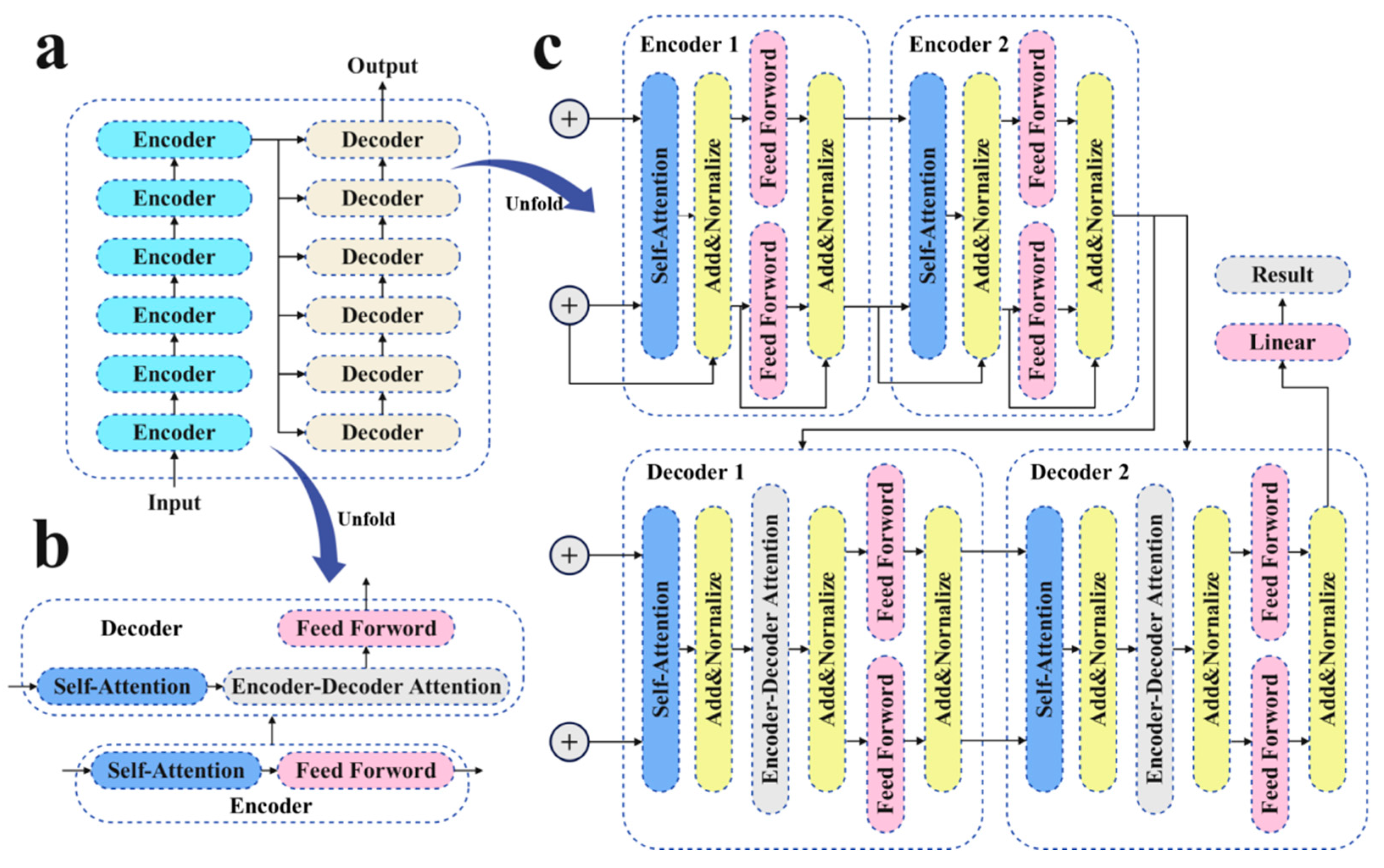
The model architecture represents a modification of standard Transformer architecture, consisting of two main components, encoders and decoders, as depicted in Figure 1. Both the encoder and decoder sections consist of six identical encoder layers. Notably, since sales forecasting deals with regression rather than classification, the Softmax layer, typically used for classification tasks in the standard Transformer model, has been omitted.
3.2. Embedding Layer
The input embedding layer plays a crucial role in transforming both the input sales history data and influencing factors for feature extraction. Essentially, embedding involves mapping from the original space to a new space with a dimension of dmodel.
Within the input embedding layer, a Linear sub-layer (also known as fully connected layers or dense layer) is employed to map features to a dmodel dimension normalized dense vector, serving as a replacement for the Word2Vec sub-layer in the original Transformer model. Simultaneously, a lookup table sub-layer is utilized to map the features related to influencing factors. The embedding results are formed through the concatenation of features from the linear sub-layer and the lookup table.
Here, Emb represents the embedding process, . “Linear” signifies the linear sub-layer process, while “Lookup” represents the process of the Lookup table sub-layer.
3.3. Positional Encoding
In addition to the traditional Sin/Cos position encoding presented in Equation (2), we incorporated Time2Vec into the Positional Encoding to encode timestamps. This addition aims to capture both periodic and non-periodic patterns in the original historical sales data.
where is the position and is the dimension,
Here, = dmodel is the dimension of Time2Vec; is the original historical sales data; is the periodic activation function; and and are learnable parameters, namely, the weight coefficients in the Time2Vec layer.
The combination of the traditional sin/cos position encoding and Time2Vec constitutes the comprehensive positional encoding results denoted as .
3.4. Encoder
Each encoder sub-layer comprises a multi-head attention sub-layer and a feedforward sub-layer. Throughout the network, a residual structure is employed, with each multi-head attention sub-layer and feedforward sub-layer followed by a residual connection and normalization sub-layer.
The input to the first encoder sub-layer is
3.4.1. Multi-Head Attention
Attention is a fundamental aspect of the Transformer, addressing the limitations of RNN’s inability to perform parallel computing and CNN’s struggle to effectively capture global information. Multi-head attention mechanisms serve as the cornerstone of the Transformer model, enabling the network to distill and extract richer feature information from various dimensions across multiple “representation sub-spaces”.
In the encoder, the multi-head attention is self-attention. Initially, each input is subject to multiplication by the three different matrices, denoted as . These matrices yield three different results, named , , and , where represents the query embedding inputs, stands for the key embedding inputs, corresponds to the value embedding inputs, dk denotes the dimension of the and , and dv refers to the dimension of the .
The next objective is to calculate the attention for each to each . This process is expressed in Equation (7).
is the self-attention matrix.
The expression of the multi-head attention mechanism is represented in Equation (8), where denotes the attention value and signifies the output weight value matrix.
where .
We call this form of attention encoder–encoder attention, which means the query, the key, and the value come from the same time series.
3.4.2. Feedforward Sub-Layer
The feedforward sub-layer, found in both the encoder and decoder sub-layers, constitutes a position-wise fully connected feedforward network (FFN). While the linear transformation remains consistent when the feedforward sub-layer is employed at various positions within the model, it is important to note that different parameters are utilized at these distinct positions.
Given the time series characteristics of the data used for sales forecasting, we have opted to substitute the ReLU activation function from the original Transformer model with ELU. This modification serves the purpose of preventing neuron inactivation during training, facilitating the handling of negative data, and ultimately enhancing the training speed.
3.4.3. Add and Norm Sub-Layer
The Add and Norm sub-layer comprises two district parts: the Add sub-layer and the Norm sub-layer. The Add sub-layer refers to the residual connection and is mathematically represented in Equation (11).
In this equation, F represents the transformation of the previous sub-layer, which could be the multi-head attention sub-layer, the feedforward sub-layer, or the masked multi-head attention sub-layer. Z represents the input. H represents the output of the Add sub-layer. This addition of the original vector ensures that the output is at least as good as the original vector.
On the other hand, the Norm sub-layer refers to normalization, and we opt for Layer Normalization instead of Batch Normalization.
Here μ denotes the mean of the input vector, while σ represents the standard deviation of the input vector. Layer normalization standardizes all elements of the input vector to have a mean of 0 and a standard deviation of 1.
Based on the above analysis, it can be derived that
3.5. Decoder
Each decoder layer includes a masked multi-head attention layer, a multi-head attention layer, and a feedforward layer. Following each of these layers, there is a residual connection and a normalization step.
3.5.1. Masked Multi-Head Attention
In contrast to the structure of the encoder layer, the decoder layer includes a masked multi-head attention layer. This masked self-attention mechanism ensures that each time step incorporates only its preceding information, simplifying attention interaction.
The mask matrix, denoted as M, has zero values along its diagonal and lower triangle elements, while its upper triangle elements are set to negative infinity ().
3.5.2. Encoder–Decoder Attention
The multi-head attention mechanism in the decoder follows the same principles as the encoder–encoder self-attention mechanism described in Section 3.4.1, with the only distinction being that the key and value are extracted from the encoder output, while the query originates from the decoder. We refer to this decoder-specific multi-head attention as “encoder-decoder attention” to differentiate it from the encoder–encoder self-attention detailed in Section 3.4.1.
The feedforward sub-layer and the Add and Norm sub-layer in the decoder mirror the structure of the encoder–encoder self-attention mechanism in the encoder.
4. Experiments
4.1. Prediction Steps
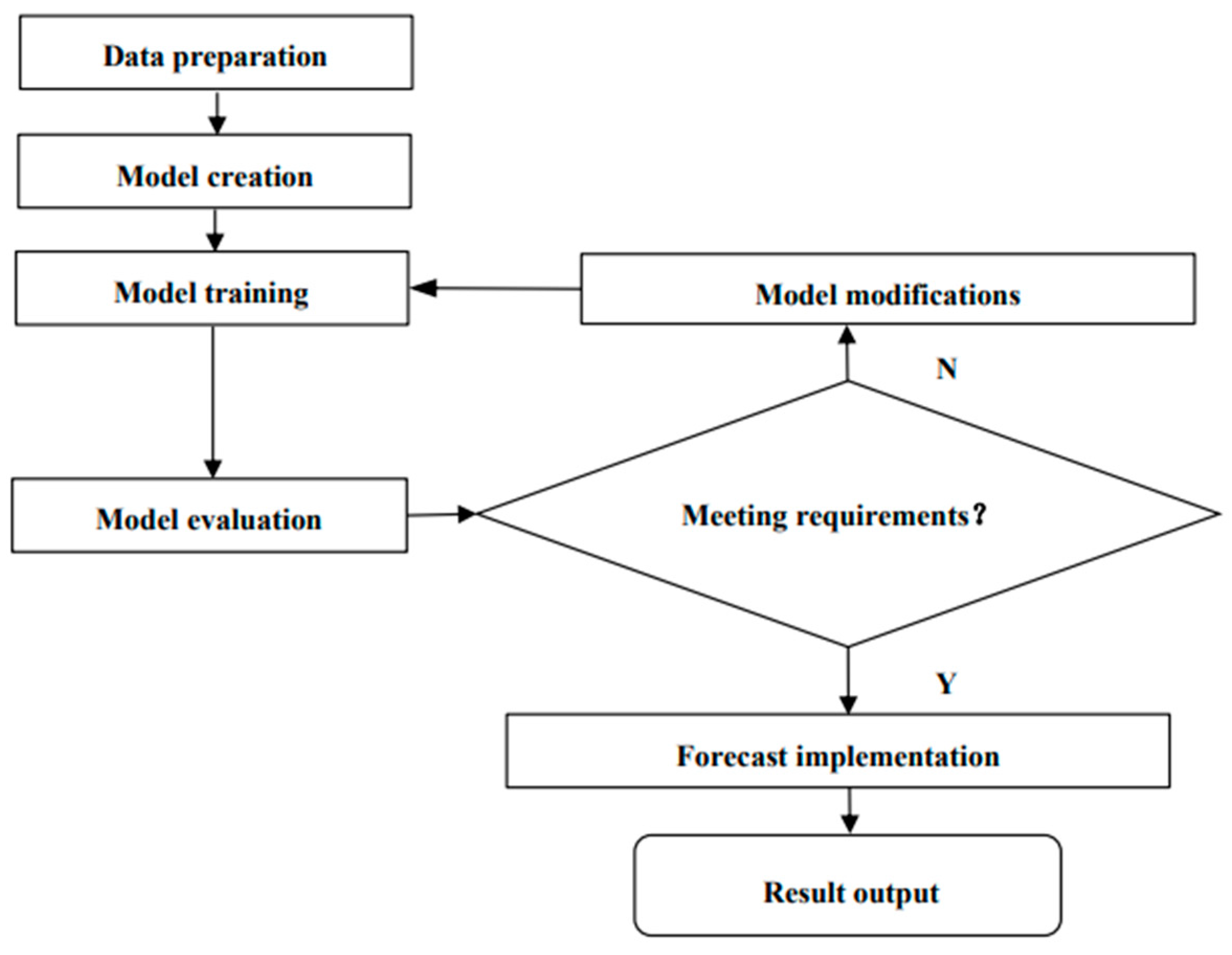
The prediction steps using the proposed Transformer model for sales forecasting are shown in Figure 2.
In the data-preparation phase, the datasets are preprocessed, encoded, and normalized, and the sub-sequence lengths and time steps are defined. During the model-creation phase, the Transformer model is built, which is described in detail in the previous section.
The model training phase and the model evaluation phase are cyclical. After the model’s training, the evaluation metrics of the model are measured and compared with other models to determine whether SOTA (state of the art) has been implemented, and the model is modified if SOTA is not reached.
The forecast-implementation phase forms the prediction results using the trained model. In the result-output phase, the forecast results are output in the form of graphs and charts to visualize the results.
4.2. Datasets and Benchmarks
We conducted the experiment using datasets from Corporación Favorita, a large grocery retailer, from 2013 to 2017, provided by Kaggle, including 125,497,040 training observation values and 3,370,464 test observation values. The datasets include train, test, stores, items, transactions, oil, and holidays_events. The data features include id, date, store_nbr, item_nbr, unit sales, onpromotion, city, state, type, cluster, family, class, durable, oil_price, etc., where id represents the unique key value; Store_nbr reports the store id, item_nbr reports the product id, onpromotion reports whether are the items in the store on that day is on sale; type represents the five store levels, A–E, and clusters representatives of similar store groups for a total of 17 groups; family is the community category, where there are a total of 33 categories, and class is the subcategory of the product, where there are 337 subcategories; durable represents whether the product easily deteriorates; oil_ price represents the oil price; and day_ type represents the type of holiday [40]. We chose training sample datasets from the dates 20170301 to 20170621, verification sample datasets from the dates 20170628 to 20170713, and test sample datasets from the dates 20170719 to 20170723. The experiment was conducted from April to July 2023.
The benchmarks employed in this study are as follows. Among them, ARMA, ARIMA, and SARIMAX represent three common traditional forecasting methods. In contrast, SVR, RNN, GRU, and LSTM are four machine-learning forecasting methods.
4.3. Experimental Settings and Model Assessment
The experiments were conducted on a computer equipped with an Intel W-2133 CPU running at 3.6 GHz, an A100 GPU, and 128 GB of RAM.
To assess the performance of proposed models and compare them with benchmarks, we selected the following evaluation metrics: RMSLE, RMSWLE, NWRMSLE, and RMALE. These metrics are defined as follows:
where represent the predicted value, denotes the true value, and N represents the number of output data points. The logarithmic component is introduced to facilitate comparison with benchmarks. These statistical measures were chosen as appropriate criteria for evaluating forecast accuracy [45].
4.4. Model Training
The dataset is partitioned into three distinct subsets: the training set, the validation set, and the prediction set. Typically, the training set comprises around 70% of the total data, while the validation set makes up approximately 20%, and the prediction set represents about 10%. We utilized the training set for model training. Throughout the model training process, we applied the Adam optimizer with the same parameters and learning rate as specified by Vaswani et al. [33]. This consistent approach ensures that our training process adheres to established standards and practices.
4.5. Experimental Results
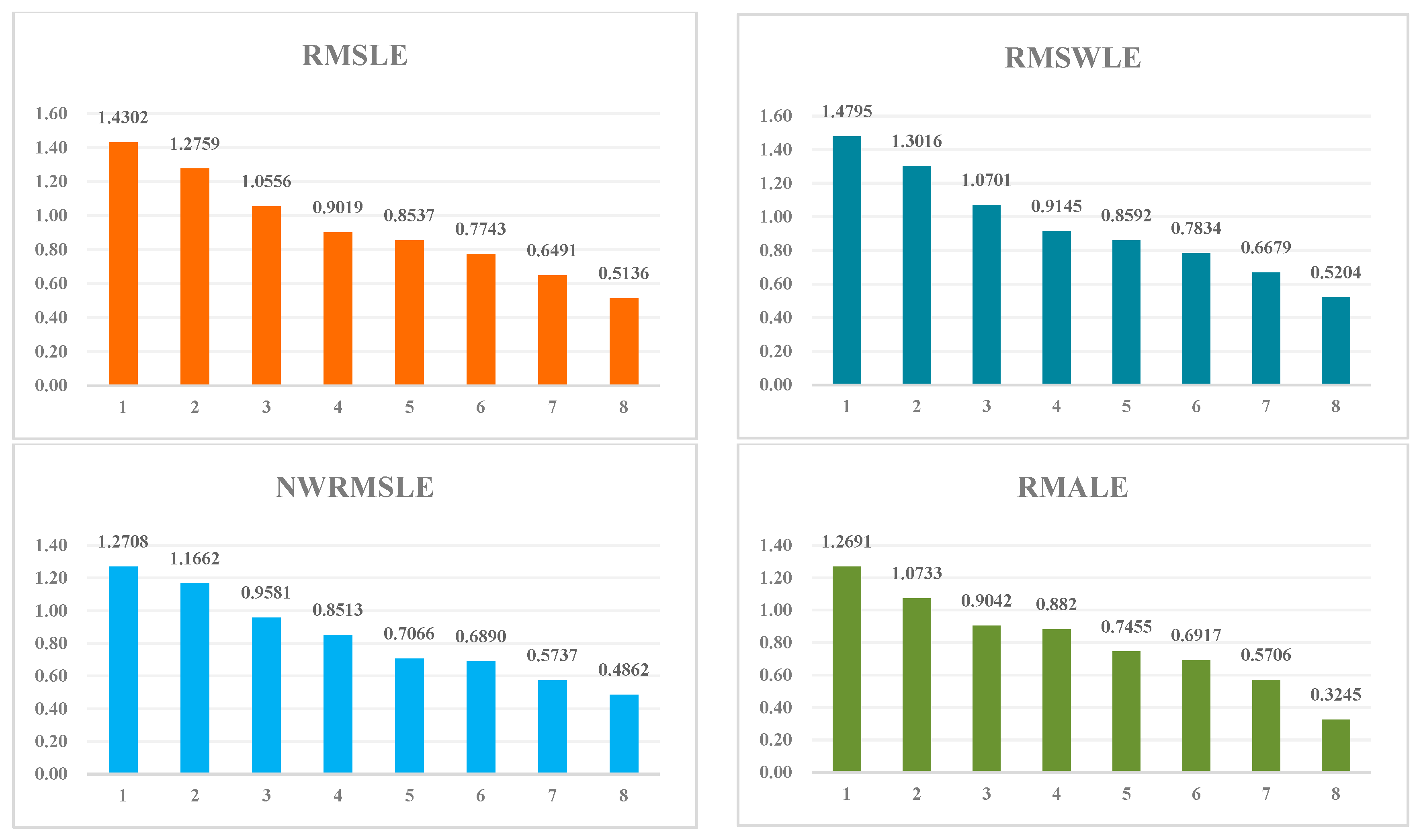
The experimental results are shown in Table 1, in which the smaller the values, the higher the prediction accuracy of the method. To provide a more intuitive and clear distinction of the predictive effects of different methods, we also visualize the table data in the form of histograms, as shown in Figure 3.
Regarding the selected model evaluation metrics RMSLE, RMSWLE, NWRMSLE, and RMALE, the proposed model exhibits average improvement rates of approximately 48.2%, 48.5%, 45.2, and 63.0%, respectively. In comparison to the traditional ARMA, ARIMA, and SARIMAX prediction models, the average improvement rates are approximately 59.1%, 59.5%, 57.0%, and 70.0%, respectively. When compared to the SVR model, the improvement rates are approximately 43.1%, 43.1%, 42.9%, and 63.2%, respectively. In contrast, when compared with the deep learning algorithm models RNN, GRU, and LSTM, the average improvement rates are approximately 32.3%, 32.4%, 25.9%, and 51.5%, respectively.
4.6. Ablation Experiment
4.6.1. Effect of Multi-Head Attention
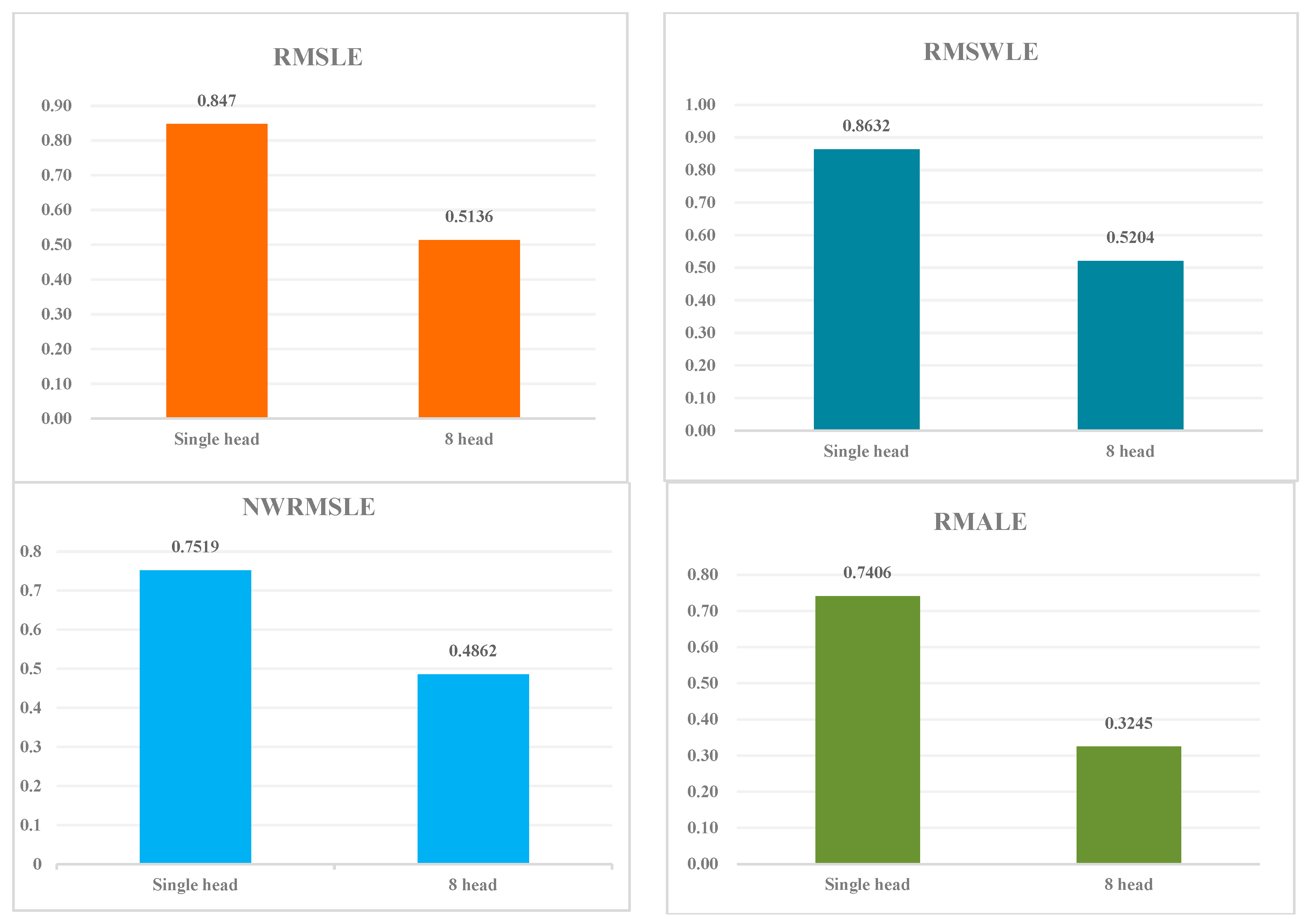
We conducted an ablation experiment to assess the impact of the multi-head attention mechanism. In comparison to the proposed model with a single-head model, the multi-head attention model exhibited average improvement of approximately 35.3%, 39.4%, 39.7%, and 56.2% on NWRMSLE, RMSLE, RMSWLE, and RMALE, respectively. Table 2 displays the results of the ablation experiment, and Figure 4 presents histograms of ablation results, clearly demonstrating that the proposed eight-head model outperforms the single-head model.
4.6.2. Effect of the Number of Encoder–Decoders
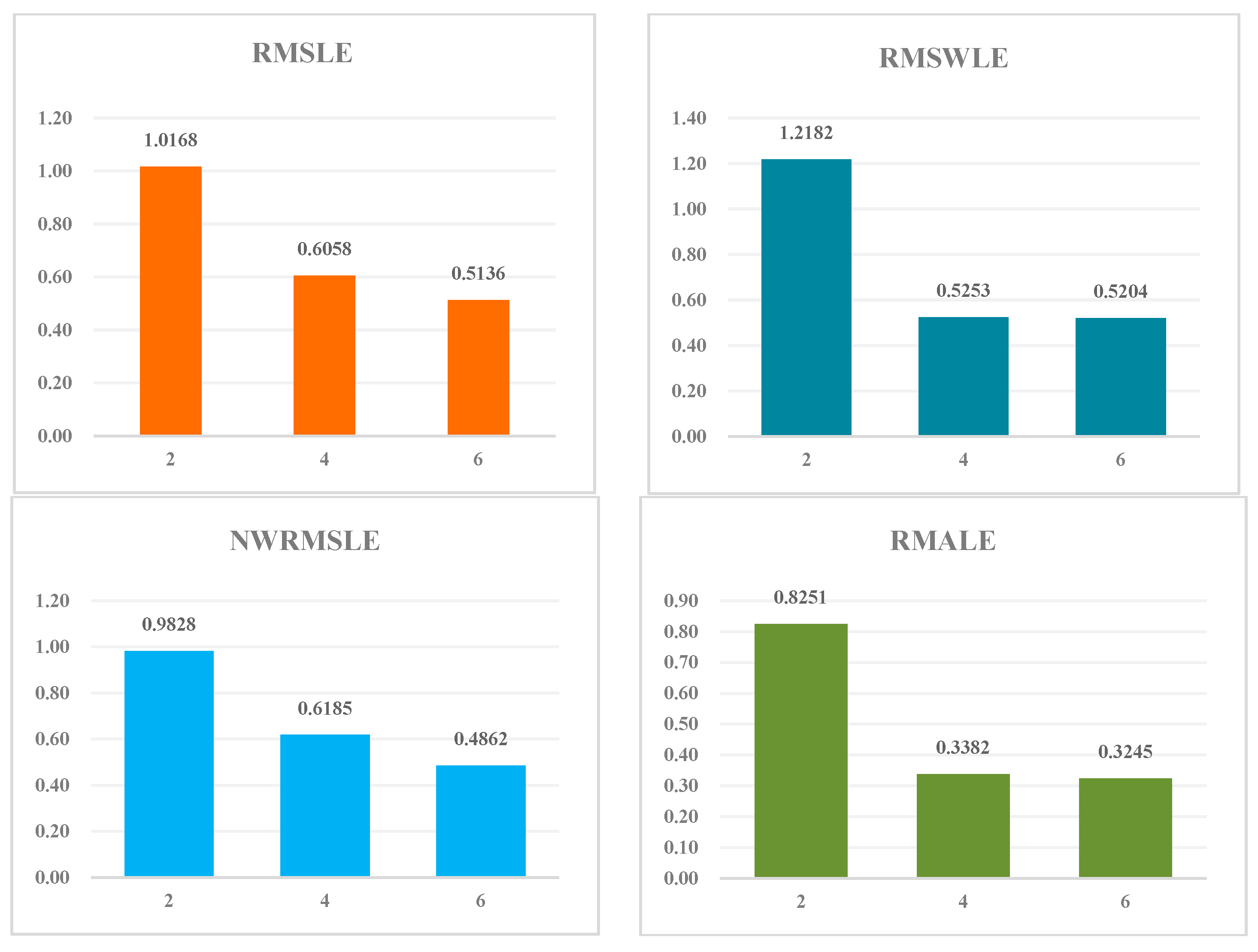
Typically, a model’s effectiveness benefits from its depth, and the deeper the model, the better its performance. The number of encoder–decoders directly corresponds to the model’s depth. Moreover, with each increment in the number of encoder–decoders, the model’s complexity increases, resulting in longer training and prediction times. Here, we assessed the impact of varying numbers of encoder–decoders on the model. The experimental results are shown in Table 3 and Figure 5. These results clearly show that as the number of encoder–decoders increases, the model’s performance improves; however, the rate of improvement diminishes. Specifically, when the number increases from 4 to 6, the enhancement in the model’s effectiveness is relatively less than when the number increases from 2 to 4. Considering the performance priority while taking into account the time efficiency comprehensively, we set the number of encoder -decoders to six.
5. Conclusions and Future Work
In the rapidly changing landscape of e-commerce, the significance of sales forecasting cannot be overstated. Unpredictable events like the COVID-19 pandemic and geopolitical conflicts have introduced unprecedented volatility into market conditions. To navigate these challenges successfully, businesses must continuously elevate their sales-forecasting capabilities to gain deeper insights and make well-informed decisions.
Our paper introduces a sales forecasting model designed to prioritize accuracy and efficiency. We leverage the Transformer’s encoder–decoder architecture and multi-head attention mechanisms to simplify long-term time-dependent computations. This not only maintains a low time complexity but also enhances the model’s interpretability. We provide a comprehensive formula representation of the model, aiding in better understanding and implementation. Our experiments on Kaggle sales datasets, considering factors like seasons, holidays, and promotions, demonstrate the model’s exceptional performance. It outperforms seven benchmark methods (ARMA, ARIMA, SARIMAX, SVR, RNN, GRU, LSTM) by approximately 48.2%, 48.5%, 45.2%, and 63.0% across four evaluation metrics (RMSLE, RMSWLE, NWRMSLE, RMALE). Ablation experiments confirm the significance of the multi-head attention mechanism and encoder–decoder layers.
Accuracy and efficiency are the basic requirements and main evaluation criteria of sales forecasting. The Transformer-based sales forecasting model proposed in this paper effectively reduces the sales forecasting error, and the average improvement rate reaches 49.1%, which is significantly higher than that of Autoformer’s 38% [37] and Fedformer’s 22.6% [38] and reaches the international advanced level. The research results fully demonstrate the superiority of our Transformer-based model.
Accuracy and efficiency are vital for sales forecasting, and our Transformer-based model excels in reducing prediction errors. Compared to traditional methods (ARMA, ARIMA, SARIMAX), it achieves improvement rates of 59.1%, 59.5%, 57.0%, and 70.0%. Compared to deep learning methods (CNN, RNN, and LSTM), it delivers improvement rates of 32.3%, 32.4%, 25.9%, and 51.5%. These results highlight the superiority of our model. Accurate sales forecasting enhances various aspects of business operations, such as production planning, pricing strategies, and inventory management, ultimately boosting sales performance and profitability. In future research endeavors, there is room for further optimization, particularly in the realm of enhancing the efficiency of the attention mechanism.
As we chart the course for future research endeavors, there remains a promising avenue for further optimization, particularly in the realm of enhancing the efficiency of the attention mechanism within our model. The attention mechanism has proven to be a powerful tool, but there is always room for refinement and streamlining to make it even more effective. When transitioning our model from research to practical enterprise settings, a critical step is to train the model using the company’s own historical sales data. While our model has demonstrated remarkable performance in our experiments, it is essential to adapt it to the unique characteristics and nuances of a specific business. Real-world data often introduce complexities that can differ significantly from standardized datasets, and this adaptation process is vital for achieving the best results.
Furthermore, the journey does not end with model development and deployment. Continuous optimization is key to maintaining and enhancing performance over time. This optimization extends to both the model itself and the fine-tuning of hyperparameters. As market conditions evolve and new factors come into play, the model should be agile and adaptable. This adaptability can be achieved through ongoing refinements based on real-world practice and feedback.
In summary, while our sales forecasting model represents a significant advancement in accuracy and efficiency, the path forward involves refining the attention mechanism, tailoring the model to specific business contexts through real-world training, and committing to continuous optimization. These steps will ensure that the model remains a valuable tool for businesses in the ever-evolving landscape of e-commerce.
Author Contributions
Conceptualization, Q.L.; methodology, Q.L.; software, Q.L.; validation, Q.L.; formal analysis, Q.L.; data curation, Q.L.; writing—original draft preparation, Q.L.; writing—review and editing, M.Y.; visualization, Q.L. All authors have read and agreed to the published version of the manuscript.
Funding
This research received no external funding.
Institutional Review Board Statement
Not applicable.
Informed Consent Statement
Not applicable.
Data Availability Statement
Data are available in a publicly accessible repository that does not issue DOIs. Publicly available datasets were analyzed in this study. These data can be found here: [https://www.kaggle.com/competitions/favorita-grocery-sales-forecasting/data (accessed on 3 April 2023)].
Acknowledgments
We acknowledged that our experiments with the model were conducted using the sales dataset provided by the Kaggle competition.
Conflicts of Interest
The authors declare no conflict of interest.
References
- Krishna, A.; Akhilesh, V.; Aich, A.; Hegde, C. Sales-forecasting of retail stores using machine learning techniques. In Proceedings of the 2018 3rd International Conference on Computational Systems and Information Technology for Sustainable Solutions (CSITSS), Bengaluru, India, 20–22 December 2018; pp. 160–166. [Google Scholar]
- Gould, P.G.; Koehler, A.B.; Ord, J.K.; Snyder, R.D.; Hyndman, R.J.; Vahid-Araghi, F. Forecasting time series with multiple seasonal patterns. Eur. J. Oper. Res. 2008, 191, 207–222. [Google Scholar] [CrossRef]
- Yan, Y.; Jiang, J.; Yang, H. Mandarin prosody boundary prediction based on sequence-to-sequence model. In Proceedings of the 2020 IEEE 4th Information Technology, Networking, Electronic and Automation Control Conference (ITNEC), Chongqing, China, 12–14 June 2020; pp. 1013–1017. [Google Scholar]
- Yu, Y.; Si, X.; Hu, C.; Zhang, J. A review of recurrent neural networks: LSTM cells and network architectures. Neural Comput. 2019, 31, 1235–1270. [Google Scholar] [CrossRef] [PubMed]
- Xie, H.H.; Li, C.; Ding, N.; Gong, C. Walmart Sale Forecasting Model Based On LSTM And LightGBM. In Proceedings of the 2021 2nd International Conference on Education, Knowledge and Information Management (ICEKIM), Xiamen, China, 29–31 January 2021; pp. 366–369. [Google Scholar]
- Joshuva, A.; Sugumaran, V. A machine learning approach for condition monitoring of wind turbine blade using autoregressive moving average (ARMA) features through vibration signals: A comparative study. Prog. Ind. Ecol. Int. J. 2018, 12, 14–34. [Google Scholar] [CrossRef]
- Efat, M.I.A.; Hajek, P.; Abedin, M.Z.; Azad, R.U.; Jaber, M.A.; Aditya, S.; Hassan, M.K. Deep-learning model using hybrid adaptive trend estimated series for modelling and forecasting sales. Ann. Oper. Res. 2022, 1–32. [Google Scholar] [CrossRef]
- Kazemi, S.M.; Goel, R.; Eghbali, S.; Ramanan, J.; Sahota, J.; Thakur, S.; Wu, S.; Smyth, C.; Poupart, P.; Brubaker, M. Time2vec: Learning a vector representation of time. arXiv 2019, arXiv:1907.05321. [Google Scholar]
- Choi, T.-M.; Yu, Y.; Au, K.-F. A hybrid SARIMA wavelet transform method for sales forecasting. Decis. Support Syst. 2011, 51, 130–140. [Google Scholar] [CrossRef]
- Abiodun, O.I.; Jantan, A.; Omolara, A.E.; Dada, K.V.; Mohamed, N.A.; Arshad, H. State-of-the-art in artificial neural network applications: A survey. Heliyon 2018, 4, e00938. [Google Scholar] [CrossRef]
- Box, G.E.; Pierce, D.A. Distribution of residual autocorrelations in autoregressive-integrated moving average time series models. J. Am. Stat. Assoc. 1970, 65, 1509–1526. [Google Scholar] [CrossRef]
- Kharfan, M.; Chan, V.W.K.; Firdolas Efendigil, T. A data-driven forecasting approach for newly launched seasonal products by leveraging machine-learning approaches. Ann. Oper. Res. 2021, 303, 159–174. [Google Scholar] [CrossRef]
- Kadam, V.; Vhatkar, S. Design and Develop Data Analysis and Forecasting of the Sales Using Machine Learning. In Intelligent Computing and Networking: Proceedings of IC-ICN 2021; Springer: Berlin/Heidelberg, Germany, 2022; pp. 157–171. [Google Scholar]
- Benvenuto, D.; Giovanetti, M.; Vassallo, L.; Angeletti, S.; Ciccozzi, M. Application of the ARIMA model on the COVID-2019 epidemic dataset. Data Brief 2020, 29, 105340. [Google Scholar] [CrossRef]
- Ampountolas, A. Modeling and forecasting daily hotel demand: A comparison based on sarimax, neural networks, and garch models. Forecasting 2021, 3, 580–595. [Google Scholar] [CrossRef]
- Montero-Manso, P.; Hyndman, R.J. Principles and algorithms for forecasting groups of time series: Locality and globality. Int. J. Forecast. 2021, 37, 1632–1653. [Google Scholar] [CrossRef]
- Berry, L.R.; Helman, P.; West, M. Probabilistic forecasting of heterogeneous consumer transaction–sales time series. Int. J. Forecast. 2020, 36, 552–569. [Google Scholar] [CrossRef]
- Ni, Y.; Fan, F. A two-stage dynamic sales forecasting model for the fashion retail. Expert Syst. Appl. 2011, 38, 1529–1536. [Google Scholar] [CrossRef]
- Junaeti, E.; Wirantika, R. Implementation of Automatic Clustering Algorithm and Fuzzy Time Series in Motorcycle Sales Forecasting. In IOP Conference Series: Materials Science and Engineering; IOP Publishing: Bristol, UK, 2018; p. 012126. [Google Scholar]
- YÜCESAN, M. Forecasting Monthly Sales of White Goods Using Hybrid Arimax and Ann Models. Atatürk Üniversitesi Sos. Bilim. Enstitüsü Derg. 2018, 22, 2603–2617. [Google Scholar]
- Parbat, D.; Chakraborty, M. A python based support vector regression model for prediction of COVID-19 cases in India. Chaos Solitons Fractals 2020, 138, 109942. [Google Scholar] [CrossRef]
- Hong, L.; Lamberson, P.; Page, S.E. Hybrid predictive ensembles: Synergies between human and computational forecasts. J. Soc. Comput. 2021, 2, 89–102. [Google Scholar] [CrossRef]
- Zhang, S.; Abdel-Aty, M.; Wu, Y.; Zheng, O. Modeling pedestrians’ near-accident events at signalized intersections using gated recurrent unit (GRU). Accid. Anal. Prev. 2020, 148, 105844. [Google Scholar] [CrossRef]
- Ma, S.; Fildes, R. Retail sales forecasting with meta-learning. Eur. J. Oper. Res. 2021, 288, 111–128. [Google Scholar] [CrossRef]
- Zhao, K.; Wang, C. Sales forecast in e-commerce using convolutional neural network. arXiv 2017, arXiv:1708.07946. [Google Scholar]
- Pham, D.-H.; Le, A.-C. Learning multiple layers of knowledge representation for aspect based sentiment analysis. Data Knowl. Eng. 2018, 114, 26–39. [Google Scholar] [CrossRef]
- Pan, H.; Zhou, H. Study on convolutional neural network and its application in data mining and sales forecasting for E-commerce. Electron. Commer. Res. 2020, 20, 297–320. [Google Scholar] [CrossRef]
- Shih, Y.-S.; Lin, M.-H. A LSTM Approach for Sales Forecasting of Goods with Short-Term Demands in E-Commerce. In Proceedings of the Intelligent Information and Database Systems: 11th Asian Conference, ACIIDS 2019, Yogyakarta, Indonesia, 8–11 April 2019; pp. 244–256. [Google Scholar]
- Wong, W.K.; Guo, Z.X. A hybrid intelligent model for medium-term sales forecasting in fashion retail supply chains using extreme learning machine and harmony search algorithm. Int. J. Prod. Econ. 2010, 128, 614–624. [Google Scholar] [CrossRef]
- Qi, Y.; Li, C.; Deng, H.; Cai, M.; Qi, Y.; Deng, Y. A deep neural framework for sales forecasting in e-commerce. In Proceedings of the 28th ACM International Conference on Information and Knowledge Management, Beijing, China, 3–7 November 2019; pp. 299–308. [Google Scholar]
- Xin, S.; Ester, M.; Bu, J.; Yao, C.; Li, Z.; Zhou, X.; Ye, Y.; Wang, C. Multi-task based sales predictions for online promotions. In Proceedings of the 28th ACM International Conference on Information and Knowledge Management, Beijing, China, 3–7 November 2019; pp. 2823–2831. [Google Scholar]
- Eachempati, P.; Srivastava, P.R.; Kumar, A.; Tan, K.H.; Gupta, S. Validating the impact of accounting disclosures on stock market: A deep neural network approach. Technol. Forecast. Soc. Chang. 2021, 170, 120903. [Google Scholar] [CrossRef]
- Vaswani, A.; Shazeer, N.; Parmar, N.; Uszkoreit, J.; Jones, L.; Gomez, A.N.; Kaiser, Ł.; Polosukhin, I. Attention is all you need. Adv. Neural Inf. Process. Syst. 2017, 30, 6000–6010. [Google Scholar]
- Qi, X.; Hou, K.; Liu, T.; Yu, Z.; Hu, S.; Ou, W. From known to unknown: Knowledge-guided transformer for time-series sales forecasting in Alibaba. arXiv 2021, arXiv:2109.08381. [Google Scholar]
- Rao, Z.; Zhang, Y. Transformer-based power system energy prediction model. In Proceedings of the 2020 IEEE 5th Information Technology and Mechatronics Engineering Conference (ITOEC), Chongqing, China, 12–14 June 2020; pp. 913–917. [Google Scholar]
- Vallés-Pérez, I.; Soria-Olivas, E.; Martínez-Sober, M.; Serrano-López, A.J.; Gómez-Sanchís, J.; Mateo, F. Approaching sales forecasting using recurrent neural networks and transformers. Expert Syst. Appl. 2022, 201, 116993. [Google Scholar] [CrossRef]
- Yoo, J.; Kang, U. Attention-based autoregression for accurate and efficient multivariate time series forecasting. In Proceedings of the 2021 SIAM International Conference on Data Mining (SDM), SIAM, Virtual, 29 April–1 May 2021; pp. 531–539. [Google Scholar]
- Yang, Y.; Lu, J. Foreformer: An enhanced transformer-based framework for multivariate time series forecasting. Appl. Intell. 2023, 53, 12521–12540. [Google Scholar] [CrossRef]
- Papadopoulos, S.-I.; Koutlis, C.; Papadopoulos, S.; Kompatsiaris, I. Multimodal Quasi-AutoRegression: Forecasting the visual popularity of new fashion products. Int. J. Multimed. Inf. Retr. 2022, 11, 717–729. [Google Scholar] [CrossRef]
- Wu, H.; Xu, J.; Wang, J.; Long, M. Autoformer: Decomposition transformers with auto-correlation for long-term series forecasting. Adv. Neural Inf. Process. Syst. 2021, 34, 22419–22430. [Google Scholar]
- Zhou, T.; Ma, Z.; Wen, Q.; Wang, X.; Sun, L.; Jin, R. Fedformer: Frequency enhanced decomposed transformer for long-term series forecasting. In Proceedings of the International Conference on Machine Learning, PMLR, Baltimore, MD, USA, 17–23 July 2022; pp. 27268–27286. [Google Scholar]
- Zhou, H.; Zhang, S.; Peng, J.; Zhang, S.; Li, J.; Xiong, H.; Zhang, W. Informer: Beyond efficient transformer for long sequence time-series forecasting. Proc. AAAI Conf. Artif. Intell. 2021, 35, 11106–11115. [Google Scholar] [CrossRef]
- Liu, S.; Yu, H.; Liao, C.; Li, J.; Lin, W.; Liu, A.X.; Dustdar, S. Pyraformer: Low-complexity pyramidal attention for long-range time series modeling and forecasting. In Proceedings of the International Conference on Learning Representations, Virtual, Vienna, Austria, 3–7 May 2021. [Google Scholar]
- Sherstinsky, A. Fundamentals of recurrent neural network (RNN) and long short-term memory (LSTM) network. Phys. D Nonlinear Phenom. 2020, 404, 132306. [Google Scholar] [CrossRef]
- Wright, D.J. Decision support oriented sales forecasting methods. J. Acad. Mark. Sci. 1988, 16, 71–78. [Google Scholar] [CrossRef]
Figure 1.
Overview of the proposed model. (a) The overall model structure adheres to the standard encoder–decoder format, with six identical encoder layers in the encoder section and six identical decoder layers in the decoder section. (b) Each encoder layer comprises two components: a self-attention layer and a feedforward layer. On the other hand, each decoder layer includes three components: a self-attention layer, a cross-attentive layer, and a feedforward layer. (c) The entire network implements a residual structure, with each self-attention layer and feedforward layer followed by a residual connection, and normalization.

Figure 2.
Steps of sales forecasting.

Figure 3.
Comparison of experiment results.

Figure 4.
Comparison of ablation experiment on the effect of multi-head attention.

Figure 5.
Effect of the number of encoder–decoders.


Table 1.
Comparison of experiment results.
| Number | Model | RMSLE | RMSWLE | NWRMSLE | RMALE |
|---|---|---|---|---|---|
| 1 | ARMA | 1.4302 ± 0.0031 | 1.4795 ± 0.0031 | 1.2708 ± 0.0032 | 1.2691 ± 0.0035 |
| 2 | ARIMA | 1.2759 ± 0.0042 | 1.3016 ± 0.0042 | 1.1662 ± 0.0041 | 1.0733 ± 0.0043 |
| 3 | SARIMAX | 1.0556 ± 0.0106 | 1.0701 ± 0.0106 | 0.9581 ± 0.0097 | 0.9042 ± 0.0109 |
| 4 | SVR | 0.9019 ± 0.0028 | 0.9145 ± 0.0028 | 0.8513 ± 0.0028 | 0.8820 ± 0.0030 |
| 5 | RNN | 0.8537 ± 0.0079 | 0.8592 ± 0.0079 | 0.7066 ± 0.0071 | 0.7455 ± 0.0081 |
| 6 | GRU | 0.7743 ± 0.0006 | 0.7834 ± 0.0006 | 0.6890 ± 0.0013 | 0.6917 ± 0.0011 |
| 7 | LSTM | 0.6491 ± 0.0010 | 0.6679 ± 0.0010 | 0.5737 ± 0.0015 | 0.5706 ± 0.0015 |
| 8 | Proposed model | 0.5136 ± 0.0014 | 0.5204 ± 0.0014 | 0.4862 ± 0.0011 | 0.3245 ± 0.0012 |
Table 2.
Effect of multi-head attention.
| Number | Model | RMSLE | RMSWLE | NWRMSLE | RMALE |
|---|---|---|---|---|---|
| 1 | Single-head | 0.8470 ± 0.0016 | 0.8632 ± 0.0016 | 0.7519 ± 0.0017 | 0.7406 ± 0.0018 |
| 2 | Proposed model (8-head) | 0.5136 ± 0.0014 | 0.5204 ± 0.0014 | 0.4862 ± 0.0011 | 0.3245 ± 0.0012 |
Table 3.
Effect of the number of encoder–decoders.
| Number of Encoder–Decoders | 2 | 4 | 6 |
|---|---|---|---|
| RMSLE | 1.0168 ± 0.0043 | 0.6058 ± 0.0092 | 0.5136 ± 0.0014 |
| RMSWLE | 1.2182 ± 0.0085 | 0.5253 ± 0.0094 | 0.5204 ± 0.0014 |
| NWRMSLE | 0.9828 ± 0.0082 | 0.6185 ± 0.0081 | 0.4862 ± 0.0011 |
| RMALE | 0.8251 ± 0.1059 | 0.3382 ± 0.0013 | 0.3245 ± 0.0012 |
Disclaimer/Publisher’s Note: The statements, opinions and data contained in all publications are solely those of the individual author(s) and contributor(s) and not of MDPI and/or the editor(s). MDPI and/or the editor(s) disclaim responsibility for any injury to people or property resulting from any ideas, methods, instructions or products referred to in the content. |
© 2023 by the authors. Licensee MDPI, Basel, Switzerland. This article is an open access article distributed under the terms and conditions of the Creative Commons Attribution (CC BY) license (https://creativecommons.org/licenses/by/4.0/).
Share and Cite
MDPI and ACS Style
Li, Q.; Yu, M. Achieving Sales Forecasting with Higher Accuracy and Efficiency: A New Model Based on Modified Transformer. J. Theor. Appl. Electron. Commer. Res. 2023, 18, 1990-2006. https://doi.org/10.3390/jtaer18040100
AMA Style
Li Q, Yu M. Achieving Sales Forecasting with Higher Accuracy and Efficiency: A New Model Based on Modified Transformer. Journal of Theoretical and Applied Electronic Commerce Research. 2023; 18(4):1990-2006. https://doi.org/10.3390/jtaer18040100
Chicago/Turabian StyleLi, Qianying, and Mingyang Yu. 2023. "Achieving Sales Forecasting with Higher Accuracy and Efficiency: A New Model Based on Modified Transformer" Journal of Theoretical and Applied Electronic Commerce Research 18, no. 4: 1990-2006. https://doi.org/10.3390/jtaer18040100