Detecting Fraudulent Transactions Using Stacked Autoencoder Kernel ELM Optimized by the Dandelion Algorithm

Abstract

The risk of fraudulent activity has significantly increased with the rise in digital payments. To resolve this issue there is a need for reliable real-time fraud detection technologies. This research introduced an innovative method called stacked autoencoder kernel extreme learning machine optimized by the dandelion algorithm (S-AEKELM-DA) to detect fraudulent transactions. The primary objective was to enhance the kernel extreme learning machine (KELM) performance by integrating the dandelion technique into a stacked autoencoder kernel ELM architecture. This study aimed to improve the overall effectiveness of the proposed method in fraud detection by optimizing the regularization parameter (c) and the kernel parameter (σ). To evaluate the S-AEKELM-DA approach; simulations and experiments were conducted using four credit card datasets. The results demonstrated remarkable performance, with our method achieving high accuracy, recall, precision, and F1-score in real time for detecting fraudulent transactions. These findings highlight the effectiveness and reliability of the suggested approach. By incorporating the dandelion algorithm into the S-AEKELM framework, this research advances fraud detection capabilities, thus ensuring the security of digital transactions.

1. Introduction

Credit cards offer numerous benefits but are also exposed to security and fraud risks such as unauthorized transactions, identity theft, skimming technology, and phishing schemes. To ensure protection, users must remain vigilant by monitoring their statements, safeguarding their personal information, relying only on trusted websites, and promptly reporting suspicious activity. However, the vulnerability of credit card information to theft on insecure internet platforms poses a significant challenge for banks and financial institutions. The unauthorized access by fraudsters, who illicitly acquire credit card and debit card details without the consumer’s knowledge or consent, results in fraudulent transactions and potential fund theft. Additionally, real-time fraud detection requires quick decision-making to prevent fraudulent transactions from being processed. The system must analyze and classify transactions rapidly while minimizing false positives and negatives [1].

Financial institutions prioritize security measures and implement robust fraud detection systems to address this issue. Artificial intelligence (AI) is a possible way to combat credit card fraud. In contrast, machine learning algorithms play a crucial role in addressing credit card fraud using linear regression, KNN, SVM, naïve Bayes, random forest, and ANN [2,3]. The design of these algorithms is to learn continuously from previous transaction data and adapt to new fraud patterns. Machine learning algorithms can determine risk levels and highlight suspicious activity by studying different parameters [4], including transaction amounts, locations, and consumer behavior.

ANN is an effective learning model with more than one hidden layer, is successful in many machine learning fields, can tackle challenging nonlinear issues, and has a robust nonlinear mapping capacity [5]. Moreover, traditional networks also have difficulties with generalization and slow learning [6].

In addition, the continuous development and improvement of ELM show superior performance in the following areas: image classification [7], text classification [8], and bioinformatics [9]. The input weights and bias are generated randomly, which directly contributes to the instability of the ELM model and has made parameter optimization for this model a popular topic.

Researchers have suggested different optimization techniques to boost ELM performance further and ensure its stability [10,11,12]. However, previous work has had some limitations if the original dataset has been complicated or highly imbalanced.

Kernel ELM (KELM) was proposed by [13] to resolve this problem. They discovered that the link weights between the hidden and input layers are unnecessary. KELM outperforms ELM in terms of performance and learning time.

The autoencoder (AE) [14] is an effective computational technique that facilitates learning data representations by replacing the input t with the input x. This method is both straightforward and efficient. Through the stacking of multiple AEs, a stacked AE (SAE) is formed, enabling the acquisition of more intricate and nuanced data representations in a structured and organized manner [14].

The dandelion algorithm (DA), inspired by dandelion sowing behavior, is a popular optimization algorithm. DA offers advantages such as a simple calculation process and ease of understanding. In DA, the dandelion’s seeding radius is dynamically modified. Meanwhile, the dandelion has a self-learning capability to guide it to sow in a better direction. DA validated its simulation performance [15] by applying 12 standard functions and comparing them with other existing algorithms, and DA performed better on the test functions. Also, DA provides good results [16] with ELM in various domains.

Our study proposed a stacked autoencoder kernel ELM optimized by the dandelion algorithm (S-AEKELM-DA). This study aimed to solve the specified machine learning objective by splitting an extensive network into multiple AE-KELM. The various AE-KELMs are stacked on different levels and connected serially. While C and σ are, respectively, the regularization factor and the kernel parameter of AE-KELM, they are randomly generated and optimized in the training phase without considering hidden nodes. Our architecture contributes to the target output for each level. The proposed stacked AE-KELM optimized by the DA presents the following advantages:

• Employing the stacked autoencoder kernel ELM makes the number of hidden nodes in each layer unimportant. It eliminates the subjective and time-consuming process of selecting the appropriate number of hidden nodes, making the model more efficient and reducing the danger of overfitting or underfitting.
• The best values of the AE-KELM parameters were adjusted using an optimization technique based on the dandelion algorithm, which was more optimal than that established using particle swarm optimization and the bat algorithm.
• Our proposed method unifies all transformation matrices into only two matrices. This unification simplifies the model’s structure and reduces storage requirements. It can also shorten the model’s execution time by minimizing computational complexity.
• According to the simulation results, the S-AEKELM-DA can achieve good testing accuracy results, including learning large amounts of data and detecting problems without causing memory problems.

Incorporating the dandelion algorithm to optimize kernel activation function and regularization parameters can improve the model’s generalization and fine-tune its performance. This optimization process helps ensure that the model is better equipped to handle the imbalanced nature of the dataset and make more accurate predictions for both the majority and minority of classes. The construction of our paper is arranged as follows. Section 2 includes brief literature on ELM and optimization techniques. A brief explanation of the dandelion optimizer and stacked kernel ELM is presented in Section 3. The description simulation tests and findings on four credit card fraud datasets are detailed in Section 4. Finally, the conclusion is outlined and future work displayed in Section 5, the concluding section.

2. Background and Related Work

Machine learning has been frequent in research projects in recent decades. It has been evaluated through a variety of data analysis phases. Various machine learning algorithms, such as decision trees, regression techniques, KNN, SVM, and network classifiers [17,18,19], are highly accurate and reliable but need a long time to understand and to label the input data.

Fabrizio Carcillo et al. [20,21] suggested the use of a hybrid strategy that enlarges the feature set of a fraud detection classifier by using unsupervised outlier scores. The development and evaluation of several granularity levels for the determination of an outlier score is what makes the contribution novel.

Roberto Saia et al. [22,23] addressed limitations of the non-balanced class distribution of data that leads towards a significant reduction of the machine learning approach performance by exploiting three different metrics of similarity to define a three-dimensional evaluation space.

Asma Cherif et al. [24] included a comprehensive overview of recent studies on identifying and forecasting fraudulent credit card transactions from 2015 to 2021. The 40 articles chosen for consideration are examined and grouped by the subjects they cover (class imbalance problem, feature engineering, etc.) and the machine learning technique they employ (conventional and deep learning modeling).

In [25], Hosein Fanai et al. proposed a two-stage framework comprised of a deep AE model as the dimensionality reduction technique, and three deep learning-based classifiers including DNN, RNN, and CNN_RNN to improve fraud detection accuracy. The Bayesian optimization algorithm is utilized to select the best hyperparameters of the employed models.

A novel network-based credit card fraud detection approach using node representation learning. CATCHM was designed by Rafael Van Belle et al. [26] to tackle the challenges of fraud detection and overcome the limitations of the current detection technique.

Additionally, ensemble learning [27,28] prevents the problem of overfitting and gives better predictions than a single model. However, the interpretability of the model is reduced due to its increased complexity; hence, the computation time is higher. In addition, much data is needed to detect the pattern, which leads to the problem of an overfitting model.

Hierarchical neural networks, such as multilayer perception and deep learning techniques, are currently very effective, but the learning process takes a long time [3,5,29,30]. As a result, our proposition that incorporates the ELM into deep architecture as an autoencoder leads to a high rate and quick learning speed. Due to hidden biases and input weights that are randomly chosen, ELM necessitates many hidden neurons, which may create a loss condition problem.

ELM with one feedforward hidden layer neural network was adopted to overcome these limitations. With little human assistance, it is a non-iterative approach, and compared to other neural network methods, ELM is special. In contrast to the backpropagation approach, it does not update a weight iteratively. However, it attributes input weights and bias randomly without being adjusted during the training phase and then automatically determines the output weights—the reasons why ELM learns rapidly [31]. Input weights are the link between input and hidden neurons, and the connections between the hidden layer and output layer neurons are known as output weights. Additionally, based on benchmarking classification and regression issues [5], it was shown that in comparison to feedforward network-based gradient-descent, the testing and validating part of many applications may now be finished quickly because the ELM algorithm attempts to offer high generalization performance in a very short time. Therefore, ELM architecture has attracted the interest of many researchers [32].

To further boost the performance of ELM, Zhu et al. [33] proposed a differential evolution-based ELM algorithm [34], which, to determine the output weights, principally uses the optimization capability of a differential evolution (DE) algorithm based on population and has a robust global optimization capability.

The EELM algorithm that Y. Wang et al. [35] proposed should theoretically result in the entire column of the hidden layer H by correctly choosing the input weights and bias before computing the output weights. It enhances the resilience property of the networks as well as the learning rate (testing accuracy, prediction accuracy, and learning time). The experimental outcomes based on both the benchmark function approximation and actual problems, such as applications for classification and regression, demonstrate the effectiveness of EELM.

Fei Han et al. [36] suggested an advanced learning algorithm called IPSO-ELM that utilizes the benefits of both PSO and ELM. The modified PSO includes both the output weights norm and the RMSE on the validation set when choosing the input weights. Compared to the E-ELM, ELM, and LM algorithms, the proposed algorithm performs better in generalization.

Diwakar Tripathi et al. [10] introduced an original activation function, and four benchmark credit-scoring datasets where a range of activation functions is employed in the simulations by employing the bat optimization technique to obtain optimum weights and biases. The findings demonstrate that the integration of bat with ELM to pre-train ELM by selecting optimum weights (between input and hidden layer) and hidden biases is better for assessing credit risk.

A novel swarm intelligence optimization algorithm called dandelion optimization DO was proposed in [37]. Unconstrained benchmark functions (CEC2017) were used to evaluate the optimization performance of DO, which was applied to four real-world problems and compared with many nature-inspired metaheuristic algorithms (nine famous algorithms) where DO verified the constrained programmability performance.

Changqing Gong et al. [15] developed an optimization technique that was dandelion-inspired. In order to compare the proposed algorithm’s performance in terms of exploration, exploitation, local optima avoidance, and convergence, twelve test functions were used. Regarding optimization accuracy and convergence speed, the results demonstrated that the DA typically finds solutions correctly and outperforms the BA, the EFWA, the GA, and the PSO on 12 benchmark functions. The outcomes of the ELM optimization further demonstrated that the DA performs well in different search regions.

ELM possesses certain limitations that require resolution. One significant drawback is the potential amplification of outcome variances acquired by classifiers in multiple trials due to the randomly generated input weights and bias.

Huang et al. proposed an enhanced iteration of ELM called kernel ELM (KELM) [13]. The researchers discovered that the connection weights between the hidden and input layers are unnecessary. KELM exhibits superior performance and quicker training speed when compared to ELM. As a result of its exceptional qualities, KELM has been successfully applied to address various practical problems [38].

Haozhen Dai et al. [39] propose two improved algorithms, ML-OCELM and MK-OCELM, for outlier and anomaly detection. ML-OCELM introduces multiple hidden layers to capture complex patterns, while MK-OCELM uses kernel functions for non-linear mapping. In experiments with benchmark databases and urban noise classification, both algorithms demonstrated superior performance compared to existing methods, highlighting their effectiveness in outlier detection.

Applying the kernel ELM model to the detection of credit card fraud was the primary goal of this work. This paper suggests an evolutionary method for generating optimum parameters of kernel ELM, such as cost parameter C and kernel parameter σ by the dandelion algorithm (DA) to resolve issues with ELM previously mentioned. We additionally suggested a stacked autoencoder kernel ELM optimized by the dandelion algorithm. A more profound overview is provided in the next part to demonstrate the success of the suggested approach.

3. Methods and Materials

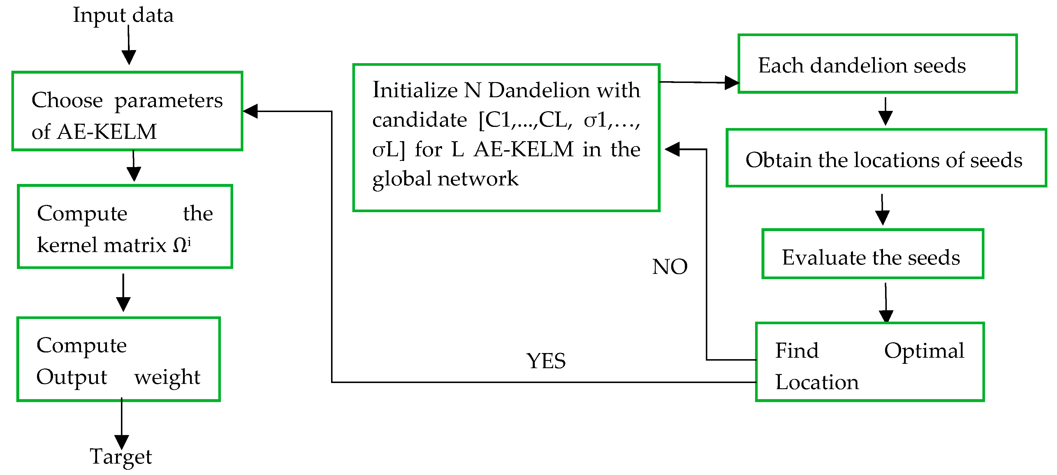
3.1. Dandelion Optimizer Algorithm

A novel swarm intelligence algorithm was created to study dandelion sowing behavior [12] and proposed for solving continuous optimization problems. Dandelion populations in DA are divided into two subpopulations: those that can be sown and those that cannot. Then, for each subgroup, different sowing strategies are applied. Meanwhile, to avoid sliding into the local optimum, another way of sowing is to conduct a subpopulation that is suited for sowing. With a dandelion, its seeds will be dispersed all around it. Dandelion seeding can be considered a hunt for an ideal in a specific area surrounding a point. This consists of the following three stages:

When seeds are in the rising stage, eddies from above cause them to rise spirally, or they may float locally in communities depending on the weather. Flying seeds continually alter their path in outer space as they fall during the descending stage. Seeds are placed in randomly chosen locations during the landing stage in order for them to grow.

Each dandelion in the population can be initialized as below:

D_i = rand × (U − L) + L

(1)

where i is an integer between 1 and the population size, rand denotes a random number between 0 and 1, dim is the dimension of the dandelion vector, and L and U are expressed as follows:

L = [l₁, …, l_dim], U = [u₁, …, u_dim]

(2)

f_best = min (f(D_i))

(3)

D_elite = D_i

Dandelion seeds must reach a certain height to separate from their parent plant during the dispersal stage. The height they rise varies depending on wind direction and air humidity. The two main parameters that influence the dispersal of dandelion seeds are wind velocity and climate. A seed’s ability to fly long or short distances depends on the wind speed [40]. Dandelion growth in nearby or remote areas is influenced by the weather, which determines whether dandelion seeds can fly. The two categories of weather that apply here are as follows:

Category 1: Wind speed distributions on a clear day can be considered lognormal distributions lnY~N (u, σ²). This distribution enhances the likelihood that dandelion seeds will spread to distant areas because random numbers are more distributed along the Y-axis. DO, therefore, prioritizes exploration in this instance. The wind scatters dandelion seeds around the search area in different directions. A dandelion seed’s increasing height is dependent on the wind speed. The higher the dandelion flies, and the farther the seeds are dispersed, the stronger is the wind. The wind speed constantly changes the vortexes above the dandelion seeds, causing them to rise in a spiral shape as follows:

$$D_{t+1}=D_t+\alpha \ast v_x\ast v_y\ast \mathrm{lnY}\ast (D_s-D_t)$$

(4)

$$D_s=\mathrm{rand} (1, \mathrm{Dim})\ast (U- L)+L$$

(5)

$$\mathrm{lnY}=\left\{\begin{array}{c}\frac{1}{y\sqrt{2\pi }}\exp \left[\frac{-1}{2{\sigma }^2}{\left(lny\right)}^2\right] y\ge 0\\ 0 y<0\end{array}\right.$$

(6)

$$\alpha =\mathrm{rand} ()\ast (\frac{1}{T^2}{t}^2-\frac{2}{T}t+1)$$

(7)

$$\mathrm{r}=\frac{1}{e^{\theta }}; v_x=r\ast \cos \theta ; v_y=r\ast \sin \theta$$

(8)

where $\theta$ is a number between $\left[-\pi , \pi \right]$.

Category 2: Because of air resistance, humidity, and other conditions, dandelion seeds cannot rise appropriately with the wind on a rainy day. Dandelion seeds are being used in this particular case in local neighborhoods, and the equivalent mathematical formula is given below:

$$D_{t+1}=D_t\ast \mathrm{k}$$

(9)

k = 1 − rand () ∗ q

(10)

$$\mathrm{q}=\mathrm{rand} ()\ast (\frac{1}{T^2-2T+1}{t}^2-\frac{1}{T^2-2T+1}t+1+\frac{1}{T^2-2T+1})$$

(11)

For dandelion seeds in their ascending stage, the mathematical expression is as follows:

$${\mathrm{X}}_{\mathrm{t}+1}=\left\{\begin{array}{c}{\mathrm{D}}_{\mathrm{t}}+\mathsf{\alpha }\ast {\mathrm{v}}_{\mathrm{x}}\ast {\mathrm{v}}_{\mathrm{y}}\ast \mathrm{lnY}\ast \left({\mathrm{D}}_{\mathrm{s}}-{\mathrm{D}}_{\mathrm{t}}\right) \mathrm{if} \mathrm{rand} \mathrm{n}<1.5\\ {\mathrm{D}}_{\mathrm{t}}\ast \mathrm{k} \mathrm{else} \end{array}\right.$$

(12)

The average position data following the rising stage reflects the dandelion descent. It helps the population grow and develop into promising communities. The corresponding mathematical formula is depicted below:

$${\mathrm{D}}_{\mathrm{t}+1}={\mathrm{D}}_{\mathrm{t}}-{\mathsf{\alpha }\ast \mathsf{\beta }}_{\mathrm{t}}\ast ({\mathrm{D}}_{\mathrm{mean}-\mathrm{t}}-\mathsf{\alpha }\ast {\mathsf{\beta }}_{\mathrm{t}}{\ast \mathrm{D}}_{\mathrm{t}})$$

(13)

In the ith iteration, ${ \mathrm{D}}_{\mathrm{mean}-\mathrm{t}}$ represents the population’s average position, and its mathematical expression is given by the following:

$$D_{mean-t}=\frac{1}{pop} {{\displaystyle \sum }}_{i=1}^{pop}{D}_i$$

(14)

Exploitation is the focus of this section of the DO algorithm. Based on the first two stages, the dandelion seed randomly decides where to land. Hopefully, the algorithm will arrive at the optimal solution as the iterations advance gradually. The approximate location where dandelion seeds will survive the most readily is the best solution that can be found. Search agents use the expert knowledge of the current elite to their advantage in their local communities to converge accurately to the global optimum. The optimal global solution will eventually be discovered through population evolution. The expression of this behavior is as follows:

$$D_{t+1}=D_{elite}+\mathrm{levy} \left(\delta \right)\ast \alpha \ast (D_{elite}-D_t\ast \mathit{\partial })$$

(15)

The dandelion seed in the ith iteration was placed in the ideal location represented by $D_{elite}$. The function of Levy flight is represented by Levy ($\delta$), which is calculated as below:

$$\mathrm{levy} (\delta )=\mathrm{s} \ast \frac{w\ast \sigma }{t^{\frac{1}{\beta }}}$$

(16)

β is a random number between (0, 2) (β = 1.25 in this paper). s is a fixed constant of 0.01, and w and t are random numbers between [0, 1]. The mathematical expression of σ is given below:

$$\sigma =\left(\frac{\Gamma \left(1+\mathsf{\beta }\right)\ast \sin (\frac{\pi \beta }{2})}{\Gamma \left(\frac{1+\mathsf{\beta }}{2}\right)\ast \mathsf{\beta }\ast 2^{\left((\beta -12)\right)}}\right)$$

(17)

$$\partial =\frac{2t}{T}$$

(18)

The algorithm ends the optimization process by setting the maximum number of iterations. The pseudocode for the proposed DO algorithm is detailed in Algorithm 1. The pseudocode for the proposed DO algorithm is detailed in Algorithm 1.

Algorithm 1 Dandelion Optimizer

Input: popsize, pop sizeim is the dimension of the variable, maximum number of iterations T, and calculate the population fitness values. Output: The best dandelion seed (Dbest) and its fitness value (best) a. Randomly initialize a population pop. b. Determine each dandelion seed’s fitness value f. c. According to fitness values, choose the best dandelion seed Delite. d. While (t < T) do Rise stage. e.        if randn () < 1.25 do f.               Use Equation (7) to produce adaptive parameters. g.                 Use Equation (4) to update dandelion seeds. h.            else if do i.                  Use Equations (10) and (11) to generate adaptive parameters. j.                  Use Equation (9) to update dandelion seeds. k.          end if Decline stage. l. Use Equation (13) to update dandelion seeds. Land stage m. Use Equation (15) to update dandelion seeds. n.  Sort dandelion seeds according to fitness values, from good to bad. o.  Update Delite p.       if f(Delite) < f(Dbest) q.             Dbest = Delite, fbest = f(Delite) r.       end if s.   end While t.   return Dbest and fbest

3.2. Kernel Extreme Learning Machine

As described by [41] ELM is a single-hidden-layer neural network that operates feed-forwardly. The input weights and hidden biases are randomly initialized, whereas the output weights are determined within a single iteration. ELM achieves good performance and fast-learning speed. To this end, ELM is used in several areas of artificial intelligence. The classical ELM algorithm is based on three steps with N training data, L hidden layer neurons, input samples X, and target matrix Y. For i = {1, 2, ……, N}, Xi ϵ Rⁿ and Yi ϵ R^c, activation function f:

(1)

Initialize randomly input weight P and hidden biases where the input nodes to the hidden layer neuron i are connected by the vector Pi = [Pi1, Pi2, …, Pin].

$$\mathrm{P}=\left[\begin{array}{c}{P}_{11} \cdots P_{1n}\\ ⋮ \ddots ⋮\\ P_{L1} \cdots P_{Ln} \end{array}\right], \mathrm{s}=\left[\begin{array}{c} s_1\\ ⋮\\ s_L \end{array}\right]$$

(19)

(2)

Calculate matrix H of output hidden layer

$$\mathrm{H}={\left[\begin{array}{c}f\left(P_1\ast X_1+s_1\right) \cdots f\left(P_L\ast X_1+s_L\right) \\ ⋮ \ddots ⋮\\ f\left(P_1\ast X_N+s_1\right) \cdots f\left(P_L\ast X_N+s_L\right) \end{array}\right]}_{N\ast L}$$

(20)

(3)

Compute output matrix weight with

O = H† ∗ Y

(21)

The Moore Penrose inverse of matrix H is denoted as H† [42,43].

The Karush–Kuhn–Tucker theory asserts [43] that the output weight O is computed as follows where C is the regularization factor:

$$O=H^T{( \frac{I}{C}+H^{T }H)}^{-1} Y$$

(22)

The output of an RBF network [44] for input data Xi ϵ Rⁿ, with R kernels will be as below:

$$\mathrm{F}(\mathrm{Xi})={{\displaystyle \sum }}_{j=1}^R{\varnothing }_j\left(Xi\right)O_j$$

(23)

For N arbitrary distinct samples (Xi, Yi) where Xi = [Xi1, Xi2, …, Xin] T Xi ϵ Rn and Yi = [Yi1, Yi2, …, Yic] T ϵ Rc, RBF can be mathematically modeled as follows:

$${{\displaystyle \sum }}_{j=1}^R{\varnothing }_j\left(Xi\right)O_j={\mathrm{T}}^{\mathrm{i}}, \mathrm{i}=1, \dots , \mathrm{N}.$$

(24)

These N samples can be approximated with zero error using standard RBF and R kernels, as in the SLFN case. That means $\Vert \mathrm{Ti}-\mathrm{Yi}\Vert$ = 0 for i = 1, …, N

$$\mathrm{H} O=H{H}^T{\left(\frac{I}{C}+H{H}^{T }\right)}^{-1} T$$

(25)

where

$$\mathsf{\Omega }={\mathrm{HH}}^{\mathrm{T}}$$

(26)

The kernel matrix was defined using a kernel function K, where Ω (i,j) = h(Xi)h(Xj) = K(Xi, Xj). Replacing HHT (9) with the kernel function, the solution can then be represented as below:

$$\mathrm{F}(\mathrm{Xi})=\left[\begin{array}{c}\mathrm{K}\left(X_i, X_1\right)\\ \mathrm{K}\left(X_i, X_2\right)\\ :\\ \mathrm{K}\left(X_i, X_N\right)\end{array}\right]{\left( \frac{I}{C}+\mathsf{\Omega }\right)}^{-1} T$$

(27)

3.3. Multilayer Extreme Learning Machines

Let Xⁱ = [$x_1^i$, …,$x_n^i$], where $x_k^i$ is the ith data representation of $x_k$ for k = 1 to n. Let ϴⁱ = [${\mathsf{ɣ}}_1^{\mathrm{i}}$, …, ${\mathsf{ɣ}}_{\mathrm{n}}^{\mathrm{i}}$] be the i th transformation matrix, where ${\mathsf{ɣ}}_k^i$, is the transformation vector used for representation learning concerning $x_k^i$.

Then, ϴi is learned by, replacing O with ϴⁱ, and Y with Xⁱ in (20):

Hⁱ ϴⁱ = Xⁱ

(28)

The output matrix of the ith hidden layer denoted as Hi, can be obtained concerning Xi using a similar approach as described in Equation (4):

$${\mathsf{ϴ}}^{\mathrm{i}}=H^{i }{\left(\frac{I}{C}+H^i{H}^{iT }\right)}^{-1} X^{i }$$

(29)

In Equation (12), ϴⁱ is utilized for representation learning, and its learning process involves multiplying $X^{i }$ with ϴⁱ:

X^final = f^N(X^N (ϴ^N)^T)

(30)

The final data representation of X, denoted as X^final, serves as the output of the hidden layer and is used to compute the output weight β in a similar manner as described in Equation (20):

X^final O = T

(31)

and O is calculated by (21)

$$\mathrm{O}=X^{final}{\left(\frac{I}{C}+X^{final}{(X^{final})}^T\right)}^{-1} T$$

(32)

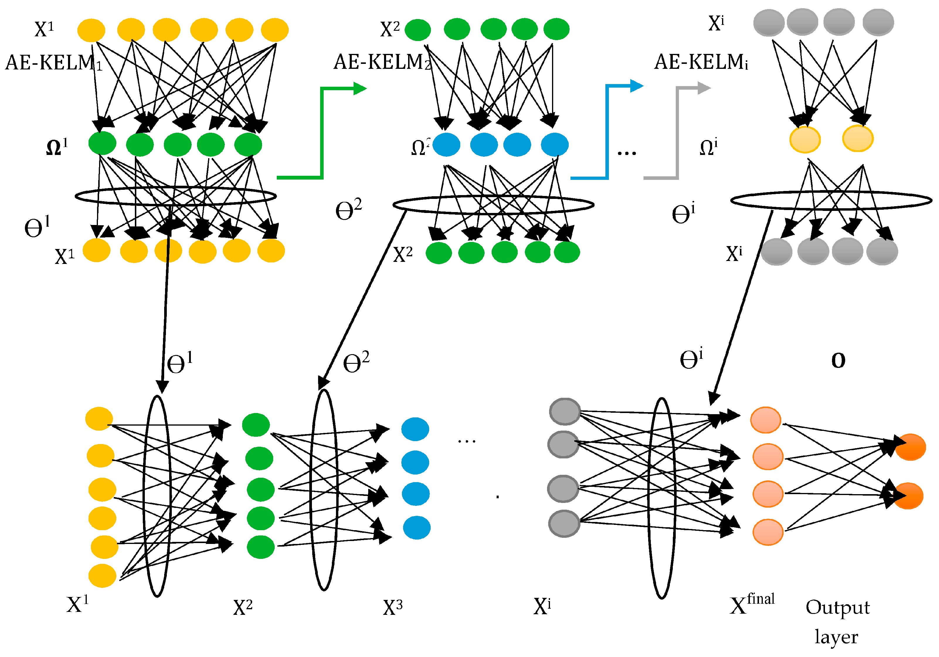
3.4. S-AEKELM-DA

Our study proposes a stacked autoencoder kernel ELM optimized by the dandelion algorithm (S-AEKELM-DA). This study aims to solve the specified machine learning objective by splitting an extensive network into multiple AE-KELM as illustrated in Algorithm 2. The various AE-KELMs are stacked on different levels and connected serially. While C and σ are, respectively, the regularization factor and the kernel parameter of AE-KELM, they are randomly generated and optimized in the training phase without considering hidden nodes.

Algorithm 2 AE-KELM

Input: input matrix Xi−1, regularization Ci−1, kernel parameters of σi−1, and activation f’i−1 Output: Xi, Ωi, ϴi Method: a.    Xi = f’i−1(Xi−1(ϴi−1)T) b.    Ωi = k(xj,xk,σi−1) c.    ϴi =${\left(\frac{I}{C_{i-1}}+{\Omega }^{i-1}\right)}^{-1}$Xi−1

In the SAE-KELM approach, every AE-KELM module is responsible for learning the data transformation from the hidden layer to the output layer, as illustrated in Figure 1 while our architecture contributes to the target output for each level. The input matrix, Xⁱ, is transformed into a kernel matrix, $\mathsf{\Omega }$ⁱ, using a kernel function. In AE-KELM, the kernel function commonly employed is the Gaussian radial basis function (RBF), expressed as follows:

$$\mathrm{K}(\mathrm{Xi}, \mathrm{Xj})=\exp (-{\Vert X_i-X_j\Vert }^2/2{\sigma }^2)$$

(33)

where σ is the kernel parameter.

The transformation matrix ϴi, denoting the ith matrix in AE-KELM, can be learned similar to ML-ELM (multi-layer extreme learning machine) in (27):

Ωⁱ ϴⁱ = Xⁱ

(34)

The final step of the transformation procedure involves obtaining the data representation Xⁱ⁺¹, which is achieved similarly in Equation (28):

Xⁱ⁺¹ = f′(Xⁱ (ϴⁱ)T)

(35)

The activation function, denoted as f’, can be chosen arbitrarily. In the case where the ith layer has the same dimension as the (i + 1) th layer, a linear piecewise activation function can be selected. In ML-KELM, all ϴⁱ have the dimension of n × n (a square matrix). As a result, the linear piecewise activation function can be applied to all ϴⁱ except for ϴ¹.

Therefore, it is possible to merge the transformation matrices ϴⁱ for i > 1 into a single matrix ϴ^unified (i > 1) without compromising the ability to represent the data accurately. As a result, all transformations can be represented using just two matrices. A detailed explanation of the S-AEKELM-DA approach can be found in Algorithm 3.

In the stage of representation learning, each pair of ϴⁱ and Xⁱ can be calculated using (28) and (17), and the Xfinal is calculated as input to train a KELM model as follows:

$${\mathsf{\Omega }}^{\mathrm{final}}\mathrm{O}=\mathrm{T}$$

(36)

and β is computed by (35)

$$\mathrm{O}={\left(\frac{I}{C}+{\mathsf{\Omega }}^{final}\right)}^{-1} T$$

(37)

Algorithm 3 Stacked AE-KELM

Input: input matrix X1, output matrix T, regularization Ci, kernel parameters of σi, the number of layers NLayer, and activation f’i Output: Hfinal matrix, two transformation matrices ϴ and ϴunified, and output weight O Method:    a. Compute the first kernel matrix Ω1(i,k) = k(xj,xk,σ1) for j, k = 1 to N    b. Calculate ϴ1 =${\left( \frac{I}{C_1}+{\Omega }^1\right)}^{-1}$X1    c. Calculate new data representation X2 = f’1(X1(ϴ1)T)    d. Compute the second kernel matrix Ω2(i,k) = k(xj,xk,σ2)    e. Calculate ϴ2 =${\left( \frac{I}{C_2}+{\Omega }^2\right)}^{-1}$X2    f. ϴunified = ϴ2    g. for i = 3: NLayer-1 do    h.   Xi, Ωi, ϴi = AE-KELM (Xi−1, Ωi−1, ϴ−1i)    i.   Update ϴunified = ϴiϴunified    j. Xfinal = XN    k. Calculate the Nth kernel matrix ΩN(i,k) = k(xj,xk,σN)    l. Calculate the output weight O =${\left( \frac{I}{C_N}+{\Omega }^N\right)}^{-1}T$

The S-AEKELM-DA learning network is made up of numerous small AE-KELM at various levels. The outputs from the hidden layers of each small AE-KELM are transmitted to the following layer via serial connections. Here, only the “optimized” kernel hidden layer outputs are passed to the following layer rather than the complete kernel hidden layer outputs. Therefore, the S-AEKELM-DA-based method can be explained as follows.

The first step in Figure 2 consists of using DA to choose the optimal C and σ in each label of the complete network. The training process of our proposed method in Figure 2 serially connects various AE-KELMs, so the optimal output weight of the first AE-KELM1 passes to the second AE-KELM² and so on until the optimal β with the best metrics is found.

As a result, a theoretically ideal reconstruction of Xⁱ is obtained (i.e., Xⁱ maintains all information of its previous data representation Xⁱ⁻¹), which explains why KELM-AE learns a superior representation for Xi. Ci is introduced to ϴⁱ in (33) to minimize overfitting, which leads to greater generalization [13]. As a result of stacking numerous KELM-AEs, S-AEKELM-DA can learn a better data representation (i.e., fewer reconstruction errors are collected and transferred to the final layer). As a result, the generalization model is improved.

Figure 2 shows the different steps of our method. First, we initialize our population with N dandelion that is chosen randomly. Each dandelion has 2L parameters to optimize, while L is the number of AE-KELM in the global network, passing with the different steps mentioned in Section 3.1.

After obtaining the best dandelion, we can compute the kernel matrix Ωⁱ for each AE-KELM to find the optimal output weight O and the target that finally is designated if the input data (transaction) is normal or not.

3.5. Other Optimization Algorithms

Bats make a brief sound pulse and then wait for a while. They determine the target object’s distance after they have received the echoes. The bat algorithm is a novel metaheuristic optimization method researchers have discovered using these bat-like characteristics [45]. A group of bats uses their ability to use echolocation to trace or hunt for food in this algorithm. Here we apply some idealized rules to optimize weight and bias, which are based on the echolocation properties of bats, to the behavior of the bats.

According to the particle swarm optimization concept [46], each particle velocity (or acceleration) is changed to move toward its pbest and gbest at each time step. Separate random numbers are generated for acceleration toward pbest and gbest, and a random term weights the acceleration.

In the case of PSO, a fixed number of particles engage in a predefined number of iterations, adjusting their positions by adding velocity vectors to their current locations.

Similarly, BA operates with a predetermined number of bats, employing echolocation and frequency tuning to alter their positions.

The mechanisms of DA, PSO, and BA exhibit distinct characteristics. Unlike other methods, DA allows a single parent to generate multiple offspring during a search process. In DA, each dandelion is capable of producing a varying number of seeds, and the subsequent iteration’s dandelions are selected from the seeds generated by different types of dandelions. The sowing and selection processes play a significant role in determining the positions of dandelions.

4. Experiments and Comparative Results

The average of 10-CV represented the experimental findings, and each fold was repeated 20 times. All algorithms and these simulations were implemented on Python 3 (Jupyter Notebook) on a PC with a 2.5 GHz CPU (Intel Core i5-7200), 12 GB RAM, and Windows (64-bit).

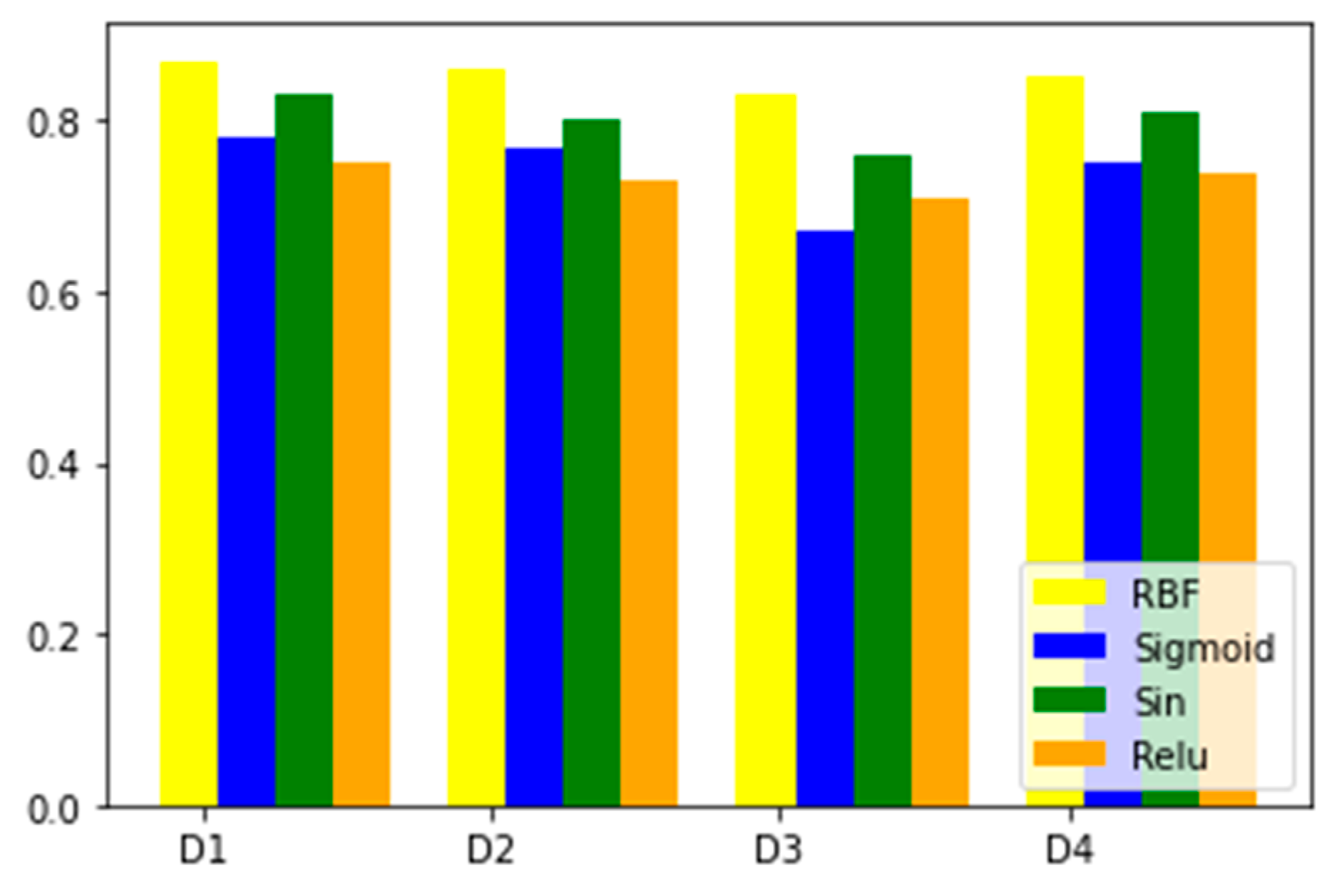
4.1. Evaluation Metrics

To evaluate the classification model on the datasets, different performance measures were computed based on the confusion matrix in

Table 1. Confusion matrix.

		Actual Transaction
		Normal(0)	Fraud (1)
Predicted Transaction	Normal(0)	True Negative TN	False Negative FN
	Fraud (1)	False Positive FP	True Positive TP

.

Accuracy is the most current parameter used, and it is defined as the ratio of all correct transactions divided by the total number of predicted transactions [47]:

$$\mathrm{Accuracy}=\frac{TN+TP}{TN+FN+FP+TP}$$

(38)

Although the dataset used is highly imbalanced, the accuracy alone will not be sufficient to calculate the performance of the model. Furthermore, other evaluation metrics [6] were used to evaluate our model, such as the following:

Recall: fraudulent transactions divided by the number of all transactions that are positive instances.

$$\mathrm{Recall} (\mathrm{Sensitivity})=\frac{TP}{TP+FN}$$

(39)

Precision: fraudulent transactions divided by the number of all transactions that are predicted as positive instances.

$$\mathrm{Precision} (\mathrm{Specificity})=\frac{TP}{TP+FP}$$

(40)

F1-score is the weighted average between recall and precision.

$$\mathrm{F}1-\mathrm{score}=2\ast \frac{Precision\ast Recall}{Precision+Recall}$$

(41)

AUC measures a learner’s merit by measuring their performance. The area of each part under the ROC curve can be added up to obtain AUC, as indicated by the definition. The AUC value increases with classification quality and, consequently, with the height of the ROC curve. The AUC value usually fluctuates between 0.5 and 1. The model’s accuracy is lower than the random results if the AUC is less than 0.5. The classification accuracy is 100% if the AUC is equal to 1, which is also the case.

4.2. Dataset

To check the effectiveness of our suggested algorithms, we select four publicly accessible datasets. They are Australian, German numerical, loan prediction, and default of credit card clients.

Table 2. Dataset information.

Dataset	Abbr.	#S	#NS	#FS	#NA	#RFS
Australian	D1	690	307	383	14	55%
German numerical	D2	1000	700	300	24	30%
Loan prediction	D3	614	422	192	12	31%
Default of credit card clients	D4	30,000	23,364	6636	24	22%

briefly shows the different information of each dataset.

Within Table 2, the column labeled “Abbr.” displays the designated codes assigned to the datasets. The “#S” entry denotes the total number of samples, while “#NS” represents the count of normal samples, and “#FS” indicates the number of fraudulent samples. Furthermore, “#NA” signifies the number of attributes present in the samples, and “#RFS” represents the ratio of fraudulent samples within a dataset.

For the D1 to D4 datasets in Figure 3, the results depict the obtained values with different activation functions, namely, rectified linear unit (Relu), radial basis function (RBF), sigmoid (Sig), and sine (Sin). According to the findings, ELM with RBF kernel function outperforms other models with various numbers of neurons. ELMs with RBF kernel consist of two user-specified parameters, the constant C and the kernel parameter σ. Also, σ is searched in a wide range {2-20, 2-9, …, 220} and C on {2-10, 2-9, …, 230}.

The training classification performance on the fourth dataset with KELM, S-AEKELM, S-AEKELM-PSO, S-AEKELM-BAT, and S-AEKELM-DA with an F1-score is shown in Figure 4.

Figure 5 shows that the best performance for S-AEKELM-DA is achieved when the number of AE-KELM components included in the model is greater than 10. Adding more than 10 AE-KELM components improves the training accuracy and potentially enhances the model’s ability to capture complex patterns and relationships in the data.

The results tabulated in

Table 3. Computing results of dataset.

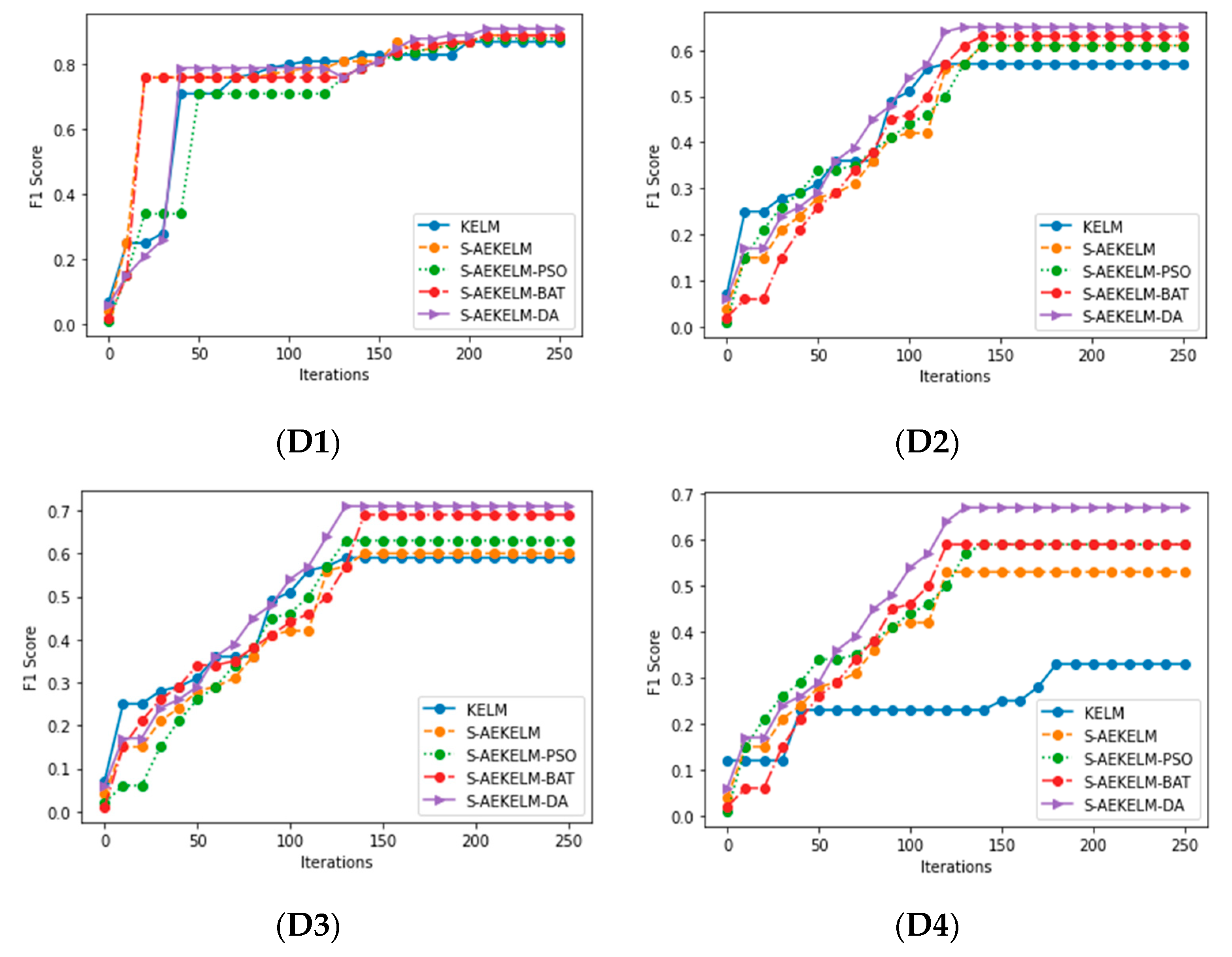
Dataset	Metric	KELM	S-AEKELM	S-AEKELM-PSO	S-AEKELM-BA	S-AEKELM-DA
D1	Acc	0.8732	0.8911	0.8889	0.8997	0.9121
	Prec	0.8747	0.8878	0.8720	0.8861	0.8945
	Recall	0.8808	0.8923	0.9047	0.9216	0.9409
	AUC	0.9129	0.9263	0.9221	0.9314	0.9568
	F1-score	0.8777	0.89	0.8873	0.9035	0.9171
D2	Acc	0.7811	0.7934	0.7916	0.8102	0.8217
	Prec	0.7331	0.7524	0.7603	0.78	0.8023
	Recall	0.9216	0.9335	0.9321	0.9347	0.9461
	AUC	0.8817	0.8864	0.8941	0.9008	0.9031
	F1-score	0.8166	0.8332	0.8374	0.8503	0.8682
D3	Acc	0.7602	0.8142	0.8211	0.8245	0.8447
	Prec	0.7809	0.7634	0.8444	0.8532	0.8602
	Recall	0.4618	0.5057	0.5132	0.5122	0.6118
	AUC	0.7913	0.7942	0.801	0.8015	0.8227
	F1-score	0.5803	0.6083	0.6384	0.6401	0.715
D4	Acc	0.7221	0.7548	0.7633	0.772	0.8322
	Prec	0.481	0.5451	0.5821	0.6016	0.753
	Recall	0.3341	0.6036	0.6009	0.5964	0.6164
	AUC	0.7011	0.7166	0.7207	0.7241	0.7633
	F1-score	0.3943	0.5729	0.5914	0.599	0.6779

represent the results obtained by the traditional KELM, S-AEKELM, S-AEKELM-PSO, S-AEKELM-BA, and S-AEKELM-DA. by applying the respective evolutionary approaches PSO, BA, and DA. From the results, it is observed that stacked-AEKELM improves classification performances as compared to KELM. It also performs better while integrating the cited evolutionary approaches, wherever S-AEKELM-DA proves exceptional results. Additionally,

Table 4. Time cost (seconds) of testing for different algorithms.

	KELM	S-AEKELM	S-AEKELM-PSO	S-AEKELM-BAT	S-AEKELM-DA
D1	25	34	37	34	38
D2	46	51	59	52	60
D3	29	33	35	32	39
D4	1417	1808	1759	1770	1783

shows the time cost of the AE-KELM using different evolutionary algorithms: PSO, BAT, and DA. The time cost of a model depends on multiple factors, including the size of the dataset, the correlation between its features, and the model architecture itself. In the case of the S-AEKELM-DA approach, including multiple hidden layers in the stacked AE-KELM contributes to a slightly higher time cost than other methods. However, it is essential to note that despite the high time cost, the S-AEKELM-DA approach demonstrates superior performance when compared to other methods such as KELM, S-AEKELM, S-AEKELM-PSO, and BAT-KELM.

Table 4 displays the time costs in seconds for testing different algorithms on four datasets (D1, D2, D3, and D4). Each column represents a different algorithm, and each row represents a different dataset. While there might be slight variations in the time costs, it appears that the three algorithms, S-AEKELM-PSO, S-AEKELM-BAT, and S-AEKELM-DA, have similar time costs for testing across the different datasets.

• N is the population size in Table 5, and the parameters are introduced as follows:
• PSO: w stands for the inertia weight, and c1 and c2 are acceleration factors.
• BA: R is the pulse emission rate, A is loudness, and α and ξ are constants.
• DA: max is the number of seeds, and X is the number of the best dandelions.

Table 5. Parameter settings.

Algorithm	Parameters
PSO	N = 50, c1 = 1.5, c2 = 1.5, w = 0.7311
BA	N = 50, A = 1, R = 1, α = γ = 0.9
DA	N = 50, X = 20, max = 100

Table 5. Parameter settings.

Algorithm	Parameters
PSO	N = 50, c1 = 1.5, c2 = 1.5, w = 0.7311
BA	N = 50, A = 1, R = 1, α = γ = 0.9
DA	N = 50, X = 20, max = 100

In

Table 6. Comparing results with previous work.

Dataset	Reference	Method	Accuracy	Recall	Precision	F1-Score	AUC
Australian	[48]	BPN	0.8683	-	-	-	-
		GP	0.87	-	-	-	-
		C4.5	0.859	-	-	-	-
		SVM + GA	0.869	-	-	-	-
	[10]	ANN	0.94	-	-	-	0.93
		KNN	0.836	-	-	-	0.893
		SVM-L	0.874	-	-	-	0.923
		SVM-R	0.861	-	-	-	0.929
		CART	0.859	-	-	-	0.894
		J48	0.845	-	-	-	0.881
		LR-R	0.862	-	-	-	0.940
	[49]	XGBoost	0.8633	0.8487	0.8449	0.8468	0.9394
		LightGBM	0.8624	0.8422	0.8476	0.8449	0.9371
		AugBoost-RP	0.8633	0.8487	0.8449	0.8468	0.9416
		AugBoost-PCA	0.8681	0.8497	0.8533	0.8515	0.9415
		AugBoost-NN	0.8645	0.8539	0.8435	0.8487	0.9424
		AugBoost-ELM	0.8635	0.8462	0.8485	0.8462	0.9422
		Our study	0.9121	0.9409	0.8945	0.9171	0.9568
German numerical	[48]	BPN	0.7783	-	-	-	-
		GP	0.781	-	-	-	-
		C4.5	0.736	-	-	-	-
		SVM + GA	0.7792	-	-	-	-
	[10]	ANN	72.80	-	-	-	75.60
		KNN	66.90	-	-	-	70.20
		SVM-L	74.80	-	-	-	79.30
		SVM-R	75.90	-	-	-	80.20
		CART	55.90	-	-	-	64.30
		J48	64.10	-	-	-	65.20
		LR-R	75.40	-	-	-	78.50
	[49]	XGBoost	0.7582	0.9208	0.7757	0.842	0.7811
		LightGBM	0.7615	0.9007	0.7887	0.841	0.7776
		AugBoost-RP	0.7519	0.8867	0.7862	0.8335	0.7707
		AugBoost-PCA	0.7605	0.8852	0.7956	0.838	0.7735
		AugBoost-NN	0.7604	0.9237	0.7766	0.8438	0.7843
		AugBoost-ELM	0.7617	0.9245	0.7775	0.8446	0.7861
		Our study	0.8217	0.9461	0.8023	0.8682	0.9031
Loan prediction	[16]	WELML	0.7883	0.5782	0.6951	0.6285	0.7311
		WELMB	0.7834	0.5834	0.6792	0.6244	0.729
		WELME	0.7867	0.5837	0.7016	0.6263	0.7317
	[50]	KNN	0.837	-	-	-	-
		SVM	0.831	-	-	-	-
		Decision Tree	0.831	-	-	-	-
		Logistic Regres	0.824	-	-	-	-
		RF	0.798	-	-	-	-
		Our study	0.8447	0.6118	0.8602	0.715	0.8227
Default of credit card clients dataset	[16]	WELML	0.7687	0.6032	0.5407	0.5683	0.7139
		WELMB	0.7657	0.6003	0.5359	0.5645	0.7110
		WELME	0.7679	0.5973	0.5391	0.5649	0.7009
	[51]	Logistic Regres	0.8139	-	-	-	-
		Decision Tree	0.8218	-	-	-	-
		Boosting	0.8235	-	-	-	-
		RF	0.8212	-s	-	-	-
		Our study	0.8322	0.6164	0.753	0.6779	0.7633

our study compared the performance of our proposed method with several existing machine learning and ensemble learning techniques on various datasets. The results consistently demonstrated that our method outperformed the other approaches regarding accuracy, recall, precision, F1-score, and AUC.

When comparing our results with machine learning methods such as BPN, GP, C4.5, SVM, KNN, and logistic regression, our method achieved higher accuracy and improved performance across all datasets. Results indicate that our approach is more effective at accurately predicting outcomes and producing reliable results.

Furthermore, our method showcased superior performance when compared to ensemble learning techniques like XGBoost, LightGBM, and AugBoost. It consistently outperformed these methods regarding accuracy, recall, precision, F1-score, and AUC, thus indicating its superiority in ensemble-based prediction tasks.

These findings highlight our proposed method’s advantages over traditional machine learning and ensemble learning techniques. Our method offers a more accurate and robust solution for various prediction and classification tasks, making it a promising approach for real-world applications.

5. Conclusions and Future Work

This paper proposed a method called S-AEKELM-DA for credit card fraud detection. This study aimed to solve the specified machine learning objective by splitting an extensive network into multiple AE-KELM. The various AE-KELMs are stacked on different levels and connected serially. While C and σ are, respectively, the regularization factor and the kernel parameter of AE-KELM, they are randomly generated and optimized in the training phase without considering hidden nodes. Several tests were conducted using four credit card fraud detection datasets to evaluate its effectiveness. The simulation results indicated that the suggested architecture gives the best findings. Furthermore, compared to KELM, S-AE-KELM, S-AE-KELM-PSO, and S-AE-KELM-BAT, S-AE-KELM-DA demonstrated higher accuracy, recall, precision, F1-score, and AUC performance criteria. Notably, S-AEKELM-DA achieved this performance advantage in a few seconds during both model training and testing phases. Thus, the proposed method was highlighted as a superior approach to detecting credit card fraud on four publicly accessible datasets with different sizes and different percentages of class imbalance. The suggested method demonstrated the effectiveness of our approach, showcasing its potential for addressing challenges in imbalanced datasets and achieving better performance compared to the literature methods. Eliminating manual tuning and optimizing the kernel function activation parameters can significantly improve the model’s ability to capture complex patterns and relationships in the data.

As future recommendations, consider the following:

• Extend the experimental evaluation of our proposed approach to a broader range of datasets with varying levels of class imbalance. It will help assess its robustness and generalizability across domains and dataset characteristics.
• Compare our approach with other state-of-the-art methods for imbalanced datasets, such as resampling techniques (e.g., SMOTE), cost-sensitive learning, or ensemble methods. It will provide insights into the relative performance and strengths of different approaches and further validate the superiority of our proposed method.
• Investigate advanced techniques for optimizing hyperparameters, such as using Bayesian optimization or evolutionary algorithms, to automatically search for optimal values of the regularization parameters C and σ. It can further enhance the performance and generalization of the model.
• Explore methods to enhance the interpretability of the model. Stacked autoencoders can sometimes be considered black-box models. Investigate techniques to extract meaningful insights from the learned representations and explain the model’s decisions.
• Apply our proposed approach to real-world applications with imbalanced datasets, such as fraud detection, medical diagnosis, or anomaly detection, to assess its practical effectiveness and impact in domains where imbalanced data is prevalent.

References

- Forough, J.; Momtazi, S. Ensemble of deep sequential models for credit card fraud detection. Appl. Soft Comput. 2021, 99, 106883. [Google Scholar] [CrossRef]
- Shen, A.; Tong, R.; Deng, Y. Application of Classification Models on Credit Card Fraud Detection. In Proceedings of the 2007 International Conference on Service Systems and Service Management, Chengdu, China, 9–11 June 2007. [Google Scholar] [CrossRef]
- Almuteer, A.H.; Aloufi, A.A.; Alrashidi, W.O.; Alshobaili, J.F.; Ibrahim, D.M. Detecting Credit Card Fraud using Machine Learning. Int. J. Interact. Mob. Technol. 2021, 15, 108–122. [Google Scholar] [CrossRef]
- Murli, D.; Jami, S.; Jog, D.; Nath, S. Credit Card Fraud Detection Using Neural Network. Int. J. Soft Comput. Eng. 2014, 2, 84–88. [Google Scholar]
- El Hlouli, F.Z.; Riffi, J.; Mahraz, M.A.; El Yahyaouy, A.; Tairi, H. Credit Card Fraud Detection Based on Multilayer Perceptron and Extreme Learning Machine Architectures. In Proceedings of the 2020 International Conference on Intelligent Systems and Computer Vision (ISCV), Fez, Morocco, 9–11 June 2020. [Google Scholar] [CrossRef]
- Ma, R.; Karimzadeh, M.; Ghabussi, A.; Zandi, Y.; Baharom, S.; Selmi, A.; Maureira-Carsalade, N. Assessment of composite beam performance using GWO–ELM metaheuristic algorithm. Eng. Comput. 2022, 38, 2083–2099. [Google Scholar] [CrossRef]
- Cao, F.; Liu, B.; Sun, D. Neurocomputing Image classification based on effective extreme learning machine. Neurocomputing 2013, 102, 90–97. [Google Scholar] [CrossRef]
- Neethu, K.S.; Jyothis, T.S.; Dev, J. Text Classification Using KM-ELM Classifier. In Proceedings of the2016 International Conference on Circuit, Power and Computing Technologies (ICCPCT), Nagercoil, India, 18–19 March 2016. [Google Scholar]
- Wang, Z.; Yu, G.; Kang, Y.; Zhao, Y.; Qu, Q. Neurocomputing Breast tumor detection in digital mammography based on extreme learning machine. Neurocomputing 2014, 128, 175–184. [Google Scholar] [CrossRef]
- Tripathi, D.; Reddy, D.; Kuppili, V.; Bablani, A. Engineering Applications of Artificial Intelligence Evolutionary Extreme Learning Machine with novel activation function for credit scoring. Eng. Appl. Artif. Intell. 2020, 96, 103980. [Google Scholar] [CrossRef]
- Shariati, M.; Mafipour, M.S.; Ghahremani, B.; Azarhomayun, F.; Ahmadi, M.; Trung, N.T.; Shariati, A. A novel hybrid extreme learning machine–grey wolf optimizer (ELM-GWO) model to predict compressive strength of concrete with partial replacements for cement. Eng. Comput. 2022, 38, 757–779. [Google Scholar] [CrossRef]
- Li, X.; Han, S.; Zhao, L.; Gong, C.; Liu, X. New Dandelion Algorithm Optimizes Extreme Learning Machine for Biomedical Classification Problems. Comput. Intell. Neurosci. 2017, 2017, 4523754. [Google Scholar] [CrossRef]
- Huang, G.; Siew, C.K. Extreme Learning Machine with Randomly Assigned RBF Kernels. Int. J. Inf. Technol. 2014, 11, 16–24. [Google Scholar]
- Lin, S.Y.; Chiang, C.C.; Li, J.-B.; Hung, Z.S.; Chao, K.M. Dynamic fine-tuning stacked auto-encoder neural network for weather forecast. Future Gener. Comput. Syst. 2018, 89, 446–454. [Google Scholar] [CrossRef]
- Gong, C.; Han, S.; Li, X.; Zhao, L.; Liu, X. A new dandelion algorithm and optimization for extreme learning machine. J. Exp. Theor. Artif. Intell. 2018, 30, 39–52. [Google Scholar] [CrossRef]
- Zhu, H.; Liu, G.; Zhou, M.; Xie, Y.; Abusorrah, A. Neurocomputing Optimizing Weighted Extreme Learning Machines for imbalanced classification and application to credit card fraud detection. Neurocomputing 2020, 407, 50–62. [Google Scholar] [CrossRef]
- Kwaku, J.; Tawiah, K.; Adoma, W.; Addai-henne, S.; Achiaa, H.; Odame, E.; Amening, S.; Eshun, J. A supervised machine learning algorithm for detecting and predicting fraud in credit card transactions. Decis. Anal. J. 2023, 6, 100163. [Google Scholar] [CrossRef]
- Roseline, J.F.; Naidu, G.; Pandi, V.S.; Alamelu, S.; Mageswari, N. Autonomous credit card fraud detection using machine learning approach☆. Comput. Electr. Eng. 2022, 102, 108132. [Google Scholar] [CrossRef]
- Bin, R.; Vitaly, S.; Paul, S. Review of Machine Learning Approach on Credit Card Fraud Detection. Hum. Centric Intell. Syst. 2022, 2, 55–68. [Google Scholar] [CrossRef]
- Carcillo, F.; Le Borgne, Y.A.; Caelen, O.; Bontempi, G. Streaming active learning strategies for real-life credit card fraud detection: Assessment and visualization. Int. J. Data Sci. Anal. 2018, 5, 285–300. [Google Scholar] [CrossRef]
- Carcillo, F.; Le Borgne, Y.A.; Caelen, O.; Kessaci, Y.; Oblé, F.; Bontempi, G. Combining unsupervised and supervised learning in credit card fraud detection. Inf. Sci. 2021, 557, 317–331. [Google Scholar] [CrossRef]
- Saia, R.; Carta, S. Evaluating credit card transactions in the frequency domain for a proactive fraud detection approach. In Proceedings of the 14th International Joint Conference on E-Business and Telecommunications (ICETE 2017), Madrid, Spain, 24–26 July 2017; Volume 4, pp. 335–342. [Google Scholar]
- Saia, R. Unbalanced data classification in fraud detection by introducing a multidimensional space analysis. In Proceedings of the 3rd International Conference on Internet of Things, Big Data and Security IoTBDS, Funchal, Portugal, 19–21 March 2018; pp. 29–40. [Google Scholar] [CrossRef]
- Cherif, A.; Badhib, A.; Ammar, H.; Alshehri, S.; Kalkatawi, M.; Imine, A. Credit card fraud detection in the era of disruptive technologies: A systematic review. J. King Saud Univ. Comput. Inf. Sci. 2023, 35, 145–174. [Google Scholar] [CrossRef]
- Fanai, H.; Abbasimehr, H. A novel combined approach based on deep Autoencoder and deep classifiers for credit card fraud detection. Expert Syst. Appl. 2023, 217, 119562. [Google Scholar] [CrossRef]
- Van Belle, R.; Baesens, B.; De Weerdt, J. CATCHM: A novel network-based credit card fraud detection method using node representation learning. Decis. Support Syst. 2023, 164, 113866. [Google Scholar] [CrossRef]
- Tanouz, D.; Subramanian, R.R.; Eswar, D.; Reddy, G.V.P.; Kumar, A.R.; Praneeth, C.H.V.N.M. Credit card fraud detection using machine learning. In Proceedings of the 2021 5th International Conference on Intelligent Computing and Control Systems (ICICCS), Madurai, India, 6–8 May 2021; pp. 967–972. [Google Scholar] [CrossRef]
- Abualigah, L. Group search optimizer: A nature-inspired meta-heuristic optimization algorithm with its results, variants, and applications. Neural Comput. Appl. 2021, 33, 2949–2972. [Google Scholar] [CrossRef]
- Ramzan, M.; Ahmed, M. Credit Card Fraud Detection Using State-of-the-Art Machine Learning and Deep Learning Algorithms. IEEE Access 2022, 10, 39700–39715. [Google Scholar] [CrossRef]
- Yu, X.; Li, X.; Dong, Y.; Zheng, R. A Deep Neural Network Algorithm for Detecting Credit Card Fraud. In Proceedings of the 2020 International Conference on Big Data, Artificial Intelligence and Internet of Things Engineering (ICBAIE), Fuzhou, China, 12–14 June 2020; pp. 181–183. [Google Scholar] [CrossRef]
- Huang, G.; Huang, G.-B.; Song, S.; You, K. Trends in extreme learning machines: A review. IEEE Access 2019, 7, 108070–108089. [Google Scholar] [CrossRef]
- Li, C.; Zhou, J.; Tao, M.; Du, K.; Wang, S.; Jahed Armaghani, D.; Tonnizam Mohamad, E. Developing hybrid ELM-ALO, ELM-LSO and ELM-SOA models for predicting advance rate of TBM. Transp. Geotech. 2022, 36, 100819. [Google Scholar] [CrossRef]
- Zhu, Q.; Qin, A.K.; Suganthan, P.N.; Huang, G. Evolutionary extreme learning machine. Pattern Recognit. 2005, 38, 1759–1763. [Google Scholar] [CrossRef]
- Yu, Y.; Gao, S.; Wang, Y.; Todo, Y. Global Optimum-Based Search Differential Evolution. IEEE/CAA J. Autom. Sin. 2019, 6, 379–394. [Google Scholar] [CrossRef]
- Wang, Y.; Cao, F.; Yuan, Y. Neurocomputing A study on effectiveness of extreme learning machine*. Neurocomputing 2011, 74, 2483–2490. [Google Scholar] [CrossRef]
- Jiang, J.; Han, F.; Ling, Q.H.; Su, B.Y. An Improved Evolutionary Extreme Learning Machine Based on Multiobjective Particle Swarm Optimization. In Intelligent Computing Methodologies; Lecture Notes in Computer Science; Springer: Cham, Switzerland, 2018; Volume 10956, pp. 1–6. [Google Scholar] [CrossRef]
- Zhao, S.; Zhang, T.; Ma, S.; Chen, M. Dandelion Optimizer: A nature-inspired metaheuristic algorithm for engineering applications. Eng. Appl. Artif. Intell. 2022, 114, 105075. [Google Scholar] [CrossRef]
- Chen, C.; Li, W.; Su, H.; Liu, K. Spectral-Spatial Classification of Hyperspectral Image Based on Kernel Extreme Learning Machine. Remote. Sens. 2014, 6, 5795–5814. [Google Scholar] [CrossRef]
- Dai, H.; Cao, J.; Wang, T.; Deng, M.; Yang, Z. Multilayer one-class extreme learning machine. Neural Netw. 2019, 115, 11–22. [Google Scholar] [CrossRef] [PubMed]
- Purschke, O.; Sykes, M.T.; Poschlod, P.; Michalski, S.G.; Römermann, C.; Durka, W.; Kühn, I.; Prentice, H.C. Interactive effects of landscape history and current management on dispersal trait diversity in grassland plant communities. J. Ecol. 2014, 102, 437–446. [Google Scholar] [CrossRef] [PubMed]
- Ding, S.; Xu, X.; Nie, R. Extreme learning machine and its applications. Neural Comput. Appl. 2014, 25, 549–556. [Google Scholar] [CrossRef]
- Serre, D. Matrices: Theory and Applications; Springer: Berlin/Heidelberg, Germany, 2002; ISBN 0387954600. [Google Scholar]
- Huang, G.-B.; Zhou, H.; Ding, X.; Zhang, R. Extreme learning machine for regression and multiclass classification. IEEE Trans. Syst. Man Cybern. Part B Cybern. 2012, 42, 513–529. [Google Scholar] [CrossRef] [PubMed]
- Huang, G.-B.; Slew, C.K. Extreme learning machine: RBF network case. In Proceedings of the ICARCV 2004 8th Control, Automation, Robotics and Vision Conference, Kunming, China, 6–9 December 2004; Volume 2, pp. 1029–1036. [Google Scholar] [CrossRef]
- Yang, X.S. A new metaheuristic Bat-inspired Algorithm. Stud. Comput. Intell. 2010, 284, 65–74. [Google Scholar] [CrossRef]
- Eberhart, R.; Kennedy, J. New optimizer using particle swarm theory. In Proceedings of the MHS’95, Proceedings of the Sixth International Symposium on Micro Machine and Human Science, Nagoya, Japan, 4–6 October 1995; pp. 39–43. [Google Scholar] [CrossRef]
- Itoo, F.; Meenakshi; Singh, S. Comparison and analysis of logistic regression, Naıve Bayes and KNN machine learning algorithms for credit card fraud detection. Int. J. Inf. Technol. 2020, 13, 1503–1511. [Google Scholar] [CrossRef]
- Huang, C.L.; Chen, M.C.; Wang, C.J. Credit scoring with a data mining approach based on support vector machines. Expert Syst. Appl. 2007, 33, 847–856. [Google Scholar] [CrossRef]
- Zou, Y.; Gao, C. Extreme Learning Machine Enhanced Gradient Boosting for Credit Scoring. Algorithms 2022, 15, 149. [Google Scholar] [CrossRef]
- Hasan, N.; Anzum, T.; Hasan, T.; Jahan, N. Machine Learning Algorithm to Predict Fraudulent Loan Requests. In Proceedings of the 12th International Conference on Computing Communication and Networking Technologies (ICCCNT), Kharagpur, India, 6–8 July 2021. [Google Scholar] [CrossRef]
- Yu, Y. The application of machine learning algorithms in credit card default prediction. In Proceedings of the 2020 International Conference on Computing and Data Science (CDS), Stanford, CA, USA, 1–2 August 2020; pp. 212–218. [Google Scholar] [CrossRef]