
Optimizing SPARQL queries over decentralized knowledge graphs
Abstract
While the Web of Data in principle offers access to a wide range of interlinked data, the architecture of the Semantic Web today relies mostly on the data providers to maintain access to their data through SPARQL endpoints. Several studies, however, have shown that such endpoints often experience downtime, meaning that the data they maintain becomes inaccessible. While decentralized systems based on Peer-to-Peer (P2P) technology have previously shown to increase the availability of knowledge graphs, even when a large proportion of the nodes fail, processing queries in such a setup can be an expensive task since data necessary to answer a single query might be distributed over multiple nodes. In this paper, we therefore propose an approach to optimizing SPARQL queries over decentralized knowledge graphs, called Lothbrok. While there are potentially many aspects to consider when optimizing such queries, we focus on three aspects: cardinality estimation, locality awareness, and data fragmentation. We empirically show that Lothbrok is able to achieve significantly faster query processing performance compared to the state of the art when processing challenging queries as well as when the network is under high load.
1.Introduction
Due to the popularity of decentralized knowledge graphs on the Web, more and increasingly large knowledge graphs encoded in RDF are becoming available [37]. Furthermore, RDF knowledge graphs made available today are becoming exceedingly large. For instance, Wikidata [70] and Bio2RDF [22] contain more than 14 billion triples each. As a result, data providers experience an increasing burden of maintaining access to the datasets; and without any monetary incentives to do so, datasets often end up becoming unavailable [4,12,67] and outdated [6].
In recent years, several decentralized systems [3,4,6,13,45,68] have been proposed to alleviate the aforementioned burden from the data providers by reducing the computational load required to keep the data available, albeit using different methods to do so. For instance, Linked Data Fragments (LDF)-based approaches [3,13,14,34,68] reduce the computational load on the server by distributing some of the query processing effort to the client, ensuring that the server only processes requests with low time complexity. On the other hand, Peer-to-Peer (P2P) systems [4,6,45] remove the centralized point of failure that a server represents and replicate the data across several nodes in a decentralized fashion, ensuring that even if the uploading node fails, the data is still accessible. For instance, RDFPeers [17] uses a structured overlay over a P2P network that relies on Dynamic Hash Tables (DHTs) to determine where to replicate certain data. However, in situations where nodes frequently leave or join the network (i.e., churn), and data is often uploaded to the network, nodes have to go through a costly adjustment process to update the overlay and redistribute the data. Instead, systems like Piqnic [4] and ColChain [6] use unstructured P2P systems as foundation, where there is no global control over where data is replicated, making the network more stable under churn.
ColChain builds upon Piqnic and divides the entire network into communities of nodes that not only replicate the same data, but also collaborate on keeping certain data (fragments) up to date. This is done by using blockchain technology [27,54,65,73] where chains of updates maintain the history of changes to the data fragments. By linking such update chains to the data fragments in a community, ColChain allows community participants to collaborate on keeping the data up-to-date while using consensus to make malicious updates less likely and allowing users to roll-back updates to an earlier version on request. Furthermore, the decentralized nature of ColChain also increases the availability of the uploaded data by replicating the data on nodes within the community.
Nevertheless, while Piqnic and ColChain already use decentralized indexes [5] to determine where data is located during query time, subgraphs needed to answer a query are usually scattered across multiple nodes. Furthermore, the indexes provide limited information that prevents the nodes from considering locality and accurately estimating join cardinalities when optimizing queries. As a result, such systems often experience an unnecessarily large amount of intermediate results when processing a query. This problem is exacerbated by the decentralized nature of the systems, since the intermediate results have to be transferred between nodes, causing a significant communication overhead.
While there are potentially many aspects to consider when optimizing queries in a decentralized setup, we will focus on three such aspects: cardinality estimation, locality awareness, and data fragmentation. Suboptimal solutions to any of these three aspects can lead to an increased communication overhead and lower performance. For instance, while fragmenting large knowledge graphs into smaller fragments ensures that nodes do not have to replicate entire knowledge graphs, using a fragmentation technique that spreads out the data relevant to a single (sub)query across several fragments can increase the communication overhead since nodes might have to send an excessive number of requests to obtain all relevant data to answer a particular query [7,8,24,39]. On the other hand, inaccurate cardinality estimations can lead to a suboptimal join strategy that increases the amount of intermediate results and therefore runtime [52,55]. And while several approaches have proposed reasonably accurate cardinality estimation techniques [52,55,57] over knowledge graphs, and for federated engines in particular [30,38,52,66], such approaches cannot easily be transferred to a decentralized setup since nodes in a decentralized setup lack a global overview of the network and the data is scattered across multiple nodes. Finally, considering locality of the data when processing queries can help ensure that larger subqueries are delegated to nodes that can process them without communicating with other nodes, lowering the data transfer overall.
Nevertheless, while an optimization approach that maximizes the degree to which entire queries can be processed by a single node could decrease the communication overhead, a study [7] found that processing entire queries on one node can actually decrease the overall performance when the network is under heavy load, and that it is equally important to balance out the query load between nodes. As such, there is a need for a more holistic approach to query optimization that is able to delegate the processing of subqueries to other nodes in the network, thus reducing the communication overhead to the extent possible. For instance, query optimization techniques that are based on star-shaped subqueries have previously been shown to increase performance by at least an order of magnitude [3,13,14,69]. This, and the fact that conjunctive subqueries are relatively efficient to process [58], means that decomposing and processing queries based on star-shaped subqueries can significantly reduce the communication overhead in decentralized systems.
In this paper, we therefore extend our work on Piqnic [4] and ColChain [6] in three aspects that work together to reduce the communication overhead when processing SPARQL queries, and in doing so, improve query processing performance in an approach that we call Lothbrok. Lothbrok adapts Characteristic Sets [3,13,14,55] to fragment data in decentralized P2P systems. Furthermore, Lothbrok builds upon Prefix-Partitioned Bloom Filters (PPBFs) [5] and proposes a new indexing scheme called Semantically Partitioned Bloom Filters (SPBFs) to obtain more accurate cardinality estimations. Lastly, Lothbrok also introduces a locality-aware query optimization strategy that takes advantage of the SPBF indexes and is able to delegate the processing of (sub)queries to neighboring nodes in the network holding relevant data.
Fig. 1.
Overview flow diagram of the contributions of Lothbrok.
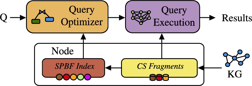
Figure 1 shows a high-level overview of the contributions of Lothbrok, following the approach described above. First, knowledge graphs are fragmented using the Characteristic Set fragmentation, and indexed using the SPBF indexes. The query optimizer uses the information available in the SPBF indexes to build a query execution plan in consideration of data locality. To obtain the final results for a given query, the execution plan is finally executed over the network.
We evaluate Lothbrok thoroughly using LargeRDFBench [61], a benchmark suite for federated RDF systems that comprises 13 datasets with over a billion triples and includes 40 queries of varying complexity and sizes of intermediate results. Furthermore, we evaluate Lothbrok using synthetic data and queries from WatDiv [9] to test the scalability of Lothbrok under load. Thus, in this paper, we focus on the query optimization problem for distributed knowledge graphs. Generalizing the approaches presented in the paper to other types of distributed graphs is an interesting topic for future work. Futhermore, the presentation of our contributions focuses on static knowledge graphs, however, updates can be managed by the underlying P2P, e.g., as done by ColChain [6]. In summary, we make the following contributions:
– A data fragmentation technique that builds on Characteristic Sets [55]
– SPBF indexes adapted to the characteristic set fragmentation technique
– A cardinality estimation approach over decentralized RDF fragments using the SPBF indexes to provide more accurate cardinality estimations
– A locality-aware query optimization algorithm that uses SPBF indexes to delegate subqueries to neighboring nodes and reduce the communication overhead
– A thorough experimental evaluation of the impact of the presented techniques on query processing performance using real-world data from a well-known benchmark suite, and large-scale synthetic datasets
The paper is structured as follows: Section 2 discusses related work while Section 3 describes background information. Then, Section 4 presents Lothbrok, Section 5 details how Lothbrok optimizes queries, and Section 6 describes the query execution approach, while Section 7 presents our experimental evaluation. Lastly, Section 8 concludes the paper with an outlook to future work.
2.Related work
The availability problem has prompted significant amount of research in the areas of decentralized query processing and decentralized architectures for knowledge graphs. In this section, we therefore discuss existing approaches related to Lothbrok; client-server architectures, federated systems, and P2P systems.
2.1.Client-server architectures
SPARQL endpoints are Web services providing an HTTP interface that accepts SPARQL queries and remain some of the most popular interfaces for querying RDF data on the Web. However, studies [12,67] have found that such endpoints are often unavailable and experience downtime.
Linked Data Fragment (LDF) interfaces, such as Triple Pattern Fragments (TPF) [68], attempt to increase the availability of the server by shifting some of the query processing load towards the client while the server only processes requests with low time complexity. For instance, TPF servers only process individual triple patterns while the TPF clients process joins and other expensive operations. Today, several TPF clients exist that rely on either a greedy algorithm [68], a metadata based strategy [36], or star-shaped query decomposition combined with adaptive query processing techniques [1] to determine the join order of the triple patterns in a query. However, while in all these approaches the server can handle more concurrent requests in comparison to SPARQL endpoints without becoming unresponsive, TPF naturally incurs a large network overhead when processing queries since intermediate bindings from previously evaluated triple patterns are transferred along with subsequently evaluated triple patterns to limit the amount of intermediate results, one by one. Furthermore, studies found that the performance of TPF is heavily affected by the type of triple pattern (i.e., the position of variables in the triple pattern) [34] and the shape of the query [50,51].
Several different systems have since been proposed to lower the network overhead. For instance, Bindings-Restricted TPF (brTPF) [32] bulks bindings from previously evaluated triple patterns such that multiple bindings can be attached to a single request. While this reduces the number of requests made for a triple pattern, it still incurs a somewhat large data transfer overhead, since each request still evaluates a single triple pattern. hybridSE [49] combines a brTPF server with a SPARQL endpoint and takes advantage of the strengths of each approach; subqueries with large numbers of intermediate results are sent to the SPARQL endpoint to overcome the limitations posed by LDF systems. However, hybridSE often answers complex queries using the SPARQL endpoint and is thus vulnerable to server failure.
To further limit the network overhead, Star Pattern Fragments (SPF) [3] clients send conjunctive subqueries in the shape of stars (star patterns) to the server and process more complex patterns locally on the client. Such conjunctive subqueries can be processed relatively efficiently by the server [58], which results in the transfer of significantly fewer intermediate results than in systems like TPF and brTPF. On the other hand, Smart-KG [14] ships predicate-family partitions (i.e., characteristic sets) to the client and processes the entire query locally; however, triple patterns with infrequent predicate values (according to a certain threshold) are sent to and evaluated by the server. While this takes advantage of the distributed resources that the clients possess, Smart-KG often ends up transferring excessive amounts of data unnecessarily since entire partitions of a dataset are transferred regardless of any bindings from previously evaluated star patterns. WiseKG [13] combines SPF and Smart-KG and uses a cost model to determine which strategy (SPF or Smart-KG) is the most cost-effective to process a given star-shaped subquery. Like SPF and Smart-KG, WiseKG processes more complex patterns on the client. Nevertheless, all the aforementioned LDF approaches rely on a centralized server or a fixed set of servers that are subject to failure.
Lastly, different from LDF approaches, SaGe [48] decreases the load on the server by suspending queries after a fixed time quantum to prevent long-running queries from exhausting server resources; the queries can then be restarted by making a new request to the server. However, SaGe processes entire, and possibly complex, queries on the server, and as stated above, such servers are subject to failure.
2.2.Federated systems
Federated systems enable answering queries over data spread out across multiple independent SPARQL endpoints [2,18,26,40,64] or LDF servers [33] offering access to different datasets. While such approaches spread out query processing over several servers, lowering the load on each individual server, they sometimes generate suboptimal query execution plans that increase the number of intermediate results and the load on individual servers [43]. As such, several approaches [30,38,52,53,62,66] have attempted to optimize federated queries in different ways. For instance, [64] builds an index over time by remembering which endpoints in the federation can provide answers to which triple patterns. Furthermore, [53] decomposes queries into subqueries that can be evaluated by a single endpoint. While [53] uses a similar query decomposition strategy as Lothbrok, they target federations over SPARQL endpoints, and as previously mentioned, such endpoints suffer from availability issues. On the other hand, [52,62] estimate the selectivity of joins to produce more efficient join plans. For instance, [52] uses characteristic sets [55] and pairs [28] to index the data in the federation and combines this with Dynamic Programming (DP) to optimize query execution plans. Furthermore, [33] proposes an interface for processing federated queries over heterogeneous LDF interfaces. To achieve this, the query optimizer is adapted to the characteristics of the different interfaces as well as the locality of the data, i.e., knowledge of which nodes hold which data. Inspired by these approaches, Lothbrok fragments knowledge graphs based on characteristic sets and uses a similar cardinality estimation technique to optimize join plans in consideration of data locality in the network.
2.3.Peer-to-peer systems
Peer-to-Peer (P2P) systems [4,6,17,24,44,45,47] tackle the availability issue from a different perspective: by removing the central point of failure completely and replicating the data across multiple nodes in a P2P network, they can ensure the data remains available even if the original node that uploaded the data fails. As such, they consist of a set of nodes (often resource limited) that act both as servers and clients, maintaining a limited local datastore. The structure of the network, i.e., connections between the nodes, as well as data placement (data allocation), varies from system to system. For instance, some systems [17,44,45] enforce data placement by applying a structured overlay over the network, such as Dynamic Hash Tables (DHTs) [46]. On the other hand, Piqnic [4] imposes no structure on top the network; nodes are connected randomly to a set of neighbors that are shuffled periodically with another node’s neighbors to increase the degree of joinability between the fragments of neighboring nodes. Lastly, ColChain [6] extends Piqnic and divides the entire network into smaller communities of nodes that collaborate on keeping certain data available and up-to-date. By applying community-based ledgers of updates and relying on a consensus protocol within a community, ColChain lets users actively participate in keeping the data up-to-date.
Each P2P system has different ways of processing queries. For instance, due to the lack of global knowledge over the network, basic P2P systems have to flood the network with requests for a given horizon to increase the likelyhood of receiving complete query results. To counteract this, distributed indexes [5,20,66] like Prefix-Partitioned Bloom Filter (PPBF) indexes [5] determine which nodes may include relevant data for a given query and thus allow the system to prune nodes from consideration during query optimization. Yet, the aforementioned systems still experience a significant overhead partly caused by inaccurate cardinality estimations, query optimization that does not consider the locality of data, as well as data fragmentation that splits up closely related data. For instance, Piqnic and ColChain both use a predicate-based fragmentation strategy that creates a fragment for each predicate. This, together with the replication and allocation strategy used, means that data relevant to a single query is distributed over a significant number of fragments and nodes.
However, while an approach that maximizes the degree to which entire queries can be processed by one node can lower the communication overhead, distributing some of the query processing load across multiple nodes is equally important when optimizing queries in a decentralized context [7] to avoid overloading individual nodes. As such, Lothbrok introduces a query optimization technique that distributes the processing of subqueries to nodes in the network based on data locality and fragment compatibility, while the characteristic set fragmentation technique allows entire star-shaped subqueries to be processed on the same node.
3.Background
A commonly used format for storing semantic data is the Resource Description Framework (RDF) [16]. RDF structures data as triples, defined as follows.
Definition 1
Definition 1(RDF Triple).
Let I, B, and L be the disjoint sets of IRIs, blank nodes, and literals. An RDF triple is a triple t of the form
Given the definition of an RDF triple, a knowledge graph
A complex BGP P can be decomposed into a set of star patterns. A star pattern
Definition 2
Definition 2(Star Decomposition [3]).
Given a BGP
The answer to a BGP P over a knowledge graph
Definition 3
Definition 3(Solution mapping [6,68]).
Given the sets I, B, L, V from above, a solution mapping μ is a partial mapping
Given a BGP P and a solution mapping μ, the notation
Since updates to the data are managed by the underlying P2P layer, solution mappings (Definition 3) are defined independently from the updating process. That is, in the general case, solution mappings are obtained on query time over the latest version of the knowledge graphs. To expand our work to support dynamic datasets, we could make use of the underlying P2P layer; if a dataset changes, the node recomputes the index and broadcasts the update throughout the network. This is what systems like ColChain [6] do, and in our experimental evaluation (Section 7) we have already implemented Lothbrok on top of ColChain. Furthermore, conflicting or inconsistent datasets in a Lothbrok network could lead to unexpected or erroneous results [72] when querying. However, the focus of this paper is on query optimization techniques and considering the quality of the datasets in Lothbrok is outside its scope. Nevertheless, in the future, we could expand Lothbrok with existing knowledge graph quality management techniques (e.g., [42,71,72]) to mitigate this problem. Thus, we refer to related work for more details on handling dynamic [6] or inconsistent [42,71,72] datasets.
3.1.Peer-to-peer
In its simplest form, an unstructured P2P system consists of a set of interconnected nodes that all maintain a local datastore managing a set of (partial) knowledge graphs, where each node maintains a local view over the network, i.e., a set of neighboring nodes and nodes reachable from those neighbors within a certain number of steps (also known as hops), called the horizon of a node.
Formally, we define a P2P network N as a set of interconnected nodes
Definition 4
Definition 4(Node [4,5]).
A node n is a triple
– G is the set of knowledge graphs in n’s local datastore
– I is n’s distributed index
– N is a set of neighboring nodes
While maintaining the structure of the network is important for P2P systems, it is not relevant for the data and query processing techniques that this paper is focusing on. As such, we do not go into detail on network topology, data replication and allocation, and periodic shuffles. Instead, we refer the interested reader to related work such as [4,6] for more details. In the following, we define data fragmentation and introduce a running example.
In line with previous work [4,6], and to avoid having to replicate large knowledge graphs throughout the network, Lothbrok divides knowledge graphs into smaller disjoint fragments, i.e., partial knowledge graphs, which can be replicated more easily. Fragments can be obtained using a fragmentation function. A fragmentation function is a function that, given a knowledge graph, returns a set of disjoint fragments, and is formally defined as follows:
Definition 5
Definition 5(Fragmentation Function [4,6]).
A fragmentation function
Different fragmentation functions can have different granularities. For instance, the most coarse-granular fragmentation function is
The fragments created by the fragmentation function are replicated and allocated at multiple nodes in the network to ensure availability in case the original provider of the knowledge graph becomes unavailable and to enable load balancing. The replication and allocation factor are parameters of the underlying network; for instance, in Piqnic [4], fragments are replicated and allocated across the node’s neighbors, and nodes index all fragments available within a certain horizon. On the other hand, ColChain [6] replicates and allocates fragments at nodes that participate within the same communities. Since this paper focuses on data fragmentation and query optimization, we omit details on data replication and allocation and refer the interested reader to related work [4,6] for details.
Fig. 2.
(a) Example of an unstructured P2P network
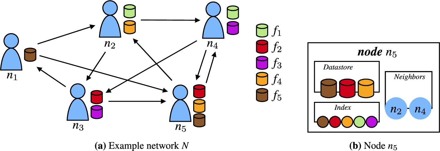
Consider, as a running example, the unstructured P2P network in Fig. 2(a) consisting of five nodes (
3.2.Distributed indexes
To speed up query processing performance, systems like Piqnic [4] and ColChain [6] use distributed indexes [5,20] to efficiently identify nodes holding relevant data for a given SPARQL query. The indexes capture information about the fragments stored locally at the node itself as well as information about fragments that can be accessed via its neighbors.
A distributed index, as defined in [5,6], is a structure that maps the triple patterns in a query to nodes that hold relevant fragments to those triple patterns. In line with [5,6], we thus define distributed indexes as follows.
Definition 6
Definition 6(Distributed Index [5,6]).
Let N be a P2P network, n be a node such that
Given a node n, n’s distributed index is denoted
Definition 7
Definition 7(Node Mapping [5,6]).
For any BPG P and distributed index I, there exists a function
To build the index for a node’s local view over the network, nodes share partial indexes, i.e., partial mappings, for the fragments that they have access to, called index slices. An index slice for a fragment is a partial mapping from triple patterns to the fragments that contain relevant triples to the triple patterns, as well as a mapping from the fragment to the nodes that replicate it, and is defined as follows:
Definition 8
Definition 8(Index Slice [5,6]).
Let f be a fragment. The index slice of f,
Index slices for the fragments that a node has access to are combined into a distributed index for that particular node using the ⊕ operator.11 The distributed index is then used to check the relevancy and overlap of fragments during query time to optimize the query. Given a set of slices S, the index obtained by combining the slices in S,
While the definition of distributed indexes allows for several different types of indexes, the index slices used in Piqnic [4] and ColChain [6] correspond to Prefix-Partitioned Bloom Filters (PPBFs) [5], which extend regular Bloom filters [15]. Given a set
To check the compatibility of two fragments relevant for conjunctive triple patterns, we check whether or not they produce any join results. To do this, we could check whether or not the intersection of the bitvectors describing the subjects and objects of the fragments is empty (i.e., if they have some IRI in common). Given two Bloom filters
To avoid exceedingly large bitvectors, PPBFs partition the bitvector based on the prefix of the IRIs. The prefix of an IRI u corresponds to the IRI of the namespace of u.22 The name of an IRI is then the IRI minus the prefix. For instance, the IRI http://dbpedia.org/resource/Denmark has the prefix (i.e., namespace IRI) http://dbpedia.org/resource/ and the name Denmark. A PPBF is formally defined in [5] as follows.
Definition 9
Definition 9(Prefix-Partitioned Bloom Filter [5]).
A PPBF
– P a set of prefixes
–
–
– H is a set of hash functions
Consider the example where the IRI dbr:Copenhagen is inserted into a PPBF, visualized in Fig. 3(a). In this case, the IRI is matched to the prefix dbr, and the name Copenhagen is hashed using each hash function in the PPBF; each corresponding bit in the bitvector for the dbr prefix is thus set to 1.
Fig. 3.
Example of (a) inserting an IRI into a PPBF
![Example of (a) inserting an IRI into a PPBF B1P and (b) intersection between two PPBFs B1P∩B2P [5].](https://content.iospress.com:443/media/sw/2023/14-6/sw-14-6-sw233438/sw-14-sw233438-g003.jpg)
Like for regular Bloom filters, we say that an IRI i with prefix p and name n may be in a PPBF
Definition 10
Definition 10(Prefix-Partitioned Bloom Filter Intersection [5]).
The intersection of two PPBFs with the same set of hash functions H and bitvectors of the same size, denoted
Consider the example intersection visualized in Fig. 3(b). As described above, the intersection of two PPBFs is the bitwise AND operation on the bitvectors for the prefixes that
Furthermore, given a partitioned bitvector
Consider, for instance, a PPBF
4.The Lothbrok approach
Differently from Piqnic and ColChain, Lothbrok uses a fragmentation strategy based on characteristic sets. To accommodate efficient query processing over such fragments, as well as to enable locality-awareness and more accurate cardinality estimation, Lothbrok introduces an indexing scheme that maps star patterns to fragments rather than triple patterns. In the remainder of this section, we provide a brief overview of the Lothbrok architecture and how Lothbrok optimizes SPARQL queries over decentralized knowledge graphs, followed by a formal definition of the fragmentation and indexing approach. Query optimization with details on how to exploit locality-awareness and join ordering are explained in Section 5.
4.1.Design and overview
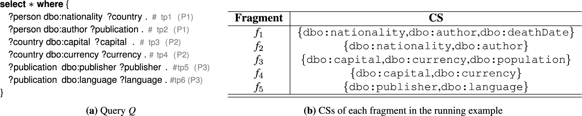
Lothbrok introduces three contributions, that altogether decrease the communication overhead and in doing so increases query processing performance. First, Lothbrok creates fragments based on characteristic sets such that entire star patterns can be answered by a single fragment. This is beneficial since, as we discussed in Section 1, such star patterns are relatively efficiently processed by the nodes [58] and reduce the communication overhead. The characteristic set of a subject value (entity) is the set of predicates that occur in triples with that subject. As such, Lothbrok creates one fragment per unique characteristic set and each fragment thus contains all the triples with the subjects that match the characteristic set of the fragment. Consider, for instance, the example network in Fig. 2 and query Q shown in Fig. 4(a). Figure 4(b) shows the characteristic sets of each fragment in the network. Using this fragmentation method, each fragment can provide answers to entire star patterns; for instance,
Fig. 4.
(a) Example SPARQL query Q and (b) corresponding characteristic sets in the example network.
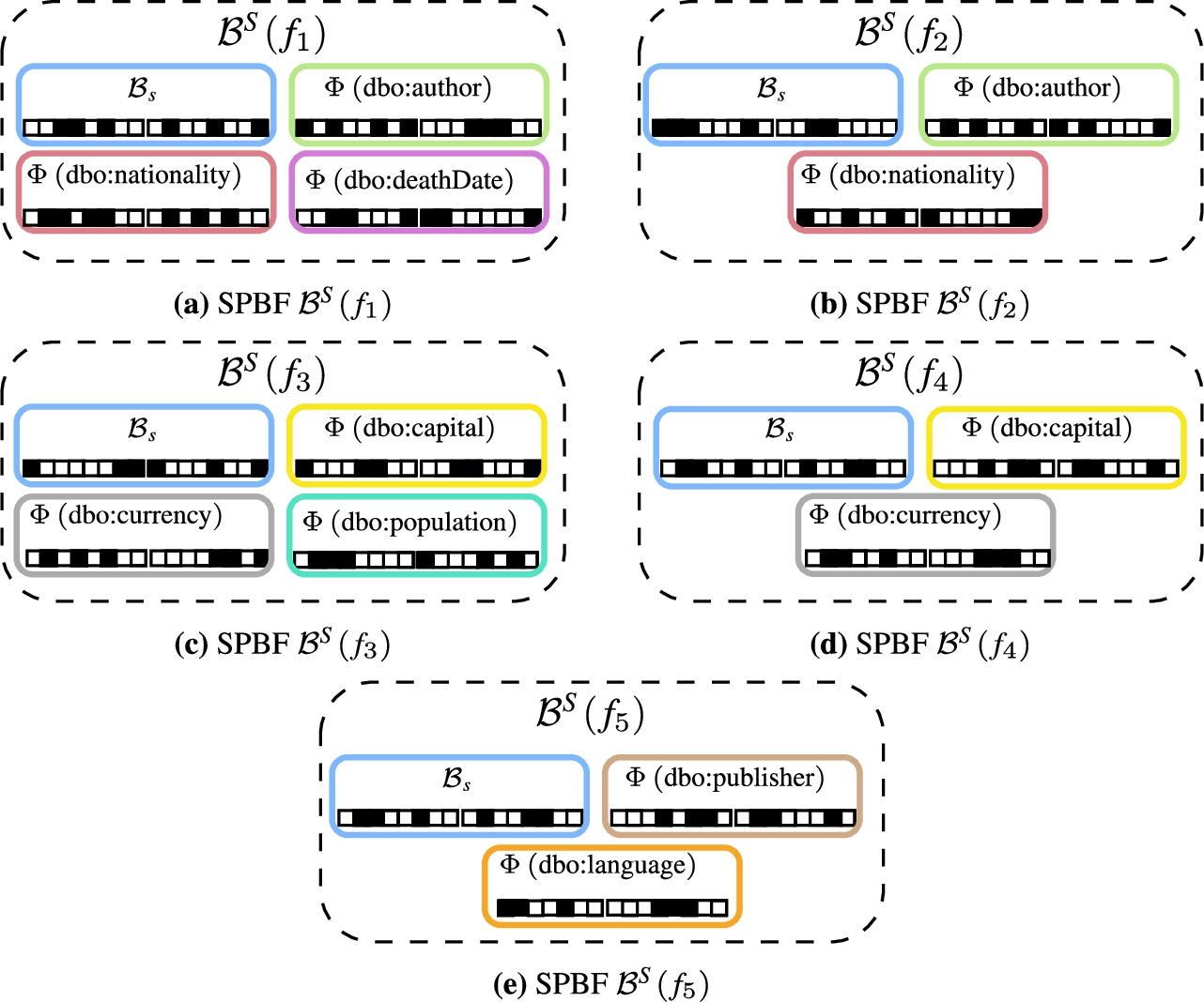
Second, to accommodate processing entire star patterns over individual fragments, and to encode structural information that can be used for cardinality estimation and locality awareness, Lothbrok introduces a novel indexing scheme, called Semantically Partitioned Bloom Filter (SPBF) Indexes, that builds upon the Prefix-Partitioned Bloom Filter (PPBF) indexes presented in [5]. In particular, SPBFs partition the bitvectors based on the IRI’s position in the fragment, i.e., whether it is a subject, predicate, or object. For instance, in the running example, the SPBF for
Third, Lothbrok proposes a query optimization technique that takes advantage of the fragmentation based on characteristic sets and the SPBF indexes to estimate cardinalities and consider data locality while optimizing the query execution plan. First, Lothbrok builds a compatibility graph using the SPBF indexes that describes, for a given query, which fragments are compatible with one another for each join in the query (i.e., which fragments may produce results for the joins). In other words, the nodes in a compatibility graph denote the relevant fragments, and the edges denote which fragments may produce join results with one another for the given query. Then, Lothbrok builds a query execution plan using a Dynamic Programming (DP) algorithm that considers the compatibility of fragments in the compatibility graph and the locality of the fragments in the index. The query execution plan built by the query optimizer follows a left-deep approach that uses the bindings obtained from previously evaluated subplans as input (filter) when processing joins. Furthermore, the plan obtained from this step includes all the relevant fragments (i.e., only non-relevant fragments are pruned).
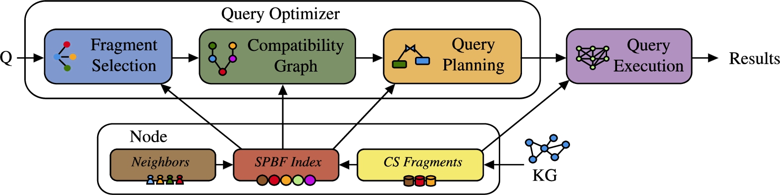
Figure 5 shows an extended version of Fig. 1 using the principles explained in Section 3.1 and the contributions explained above. The query optimizer thus contains three sequential steps; (1) fragment selection, (2) compatibility graph, and (3) query planning, that altogether computes the query execution plan for a given query.
Notice that for star patterns P with a large number of solution mappings,
In the remainder of this section, we detail data fragmentation (Section 4.2) and indexing (Section 4.3) in Lothbrok. Section 5 details the query optimization approach used by Lothbrok.
4.2.Data fragmentation
As discussed in Section 1, star-shaped subqueries can be processed relatively efficiently over a fragment [58], thus they can also help achieving a better balance between reducing the communication overhead and distributing the query processing load [3,13,14]. To facilitate processing such star patterns on single nodes, we propose to fragment the uploaded knowledge graphs based on characteristic sets [13,14,55]. This is the first contribution as explained in Section 4.1, and corresponds to the CS Fragments step in Fig. 5. Formally, a characteristic set is defined as follows:
Definition 11
Definition 11(Characteristic Set [13,14,55]).
The characteristic set for a subject s in a given knowledge graph
In other words, the characteristic set of a subject is the set of predicates (i.e., predicate combination) used to describe the subject, i.e., that occur in the same triples as the subject. For instance, if the triples (dbr:Denmark,dbo:capital,dbr:Copenhagen) and (dbr:Denmark,dbo:currency,dbr:Danish_Krone) are the only ones with subject dbr:Denmark, then this subject is described by the characteristic set {dbo:capital,dbo:currency}.
Characteristic sets were first introduced in [55], used for cardinality estimation and, in extension of that, join ordering. WiseKG [13] and Smart-KG [14] used the notion of characteristic sets for fragmentation of knowledge graphs in LDF systems to balance the query load between clients and servers. In this paper, we use characteristic set based fragments as an alternative to the purely predicate-based fragmentation used by for example Piqnic. We define the characteristic set based fragmentation function as follows:
Definition 12
Definition 12(Characteristic Set Fragmentation Function).
Let
That is, the characteristic set fragmentation function creates a fragment for each characteristic set in the knowledge graph. In the characteristic sets shown in Fig. 4(b),
Depending on the complexity of the knowledge graph, however, using fragmentation purely based on characteristic sets can quickly lead to an unwieldy number of fragments. In our experimental evaluation in Section 7, fragmenting the data from LargeRDFBench [61] using Equation (3) led to 181,859 distinct fragments most of which contain very few subjects. Consider, for instance, in the running example, the situation where the following five characteristic sets are found in the uploaded knowledge graph; for illustration purposes we have extended the notation with the number of subjects covered by each characteristic set:
The fragments in the above example are skewed with a significant difference between the largests and smallest fragments. For instance, a separate fragment is created for
To partially address the data skew issue, we merge fragments with infrequent characteristic sets into fragments with more frequent characteristic sets, similar to [55]. While such an approach potentially has the tradeoff that some of the information in the merged fragments is lost, which could in rare cases lead to incomplete query results, we did not encounter such incomplete results in our experimental evaluation (Section 7). After fragmenting datasets using Equation (3), we iteratively merge the fragments with the lowest number of distinct subject values into other fragments until the total number of fragments is below a threshold, or all fragments with fewer subject values than a threshold have been merged, using the following strategy. In our experiments (Section 7), we computed two sets of fragments for each dataset; one where the total number of fragments matched the number of predicate-based fragments, and one where all fragments with fewer than 50 subjects (determined empirically based on the data used in our experiments) were merged.
First, for infrequent fragments
Second, the remaining fragments f, i.e., ones that cannot directly be merged into any frequent fragments, are split into a set of disjoint fragments,
The steps above are sequential, i.e., all fragments that can be merged into other fragments without splitting are merged according to the first step, whereas the remaining infrequent fragments afterwards have to be split and merged according to the second step. In the example above, we end up with the following fragments:
Clearly, the data skew caused by the fragmentation approach is affected by the structuredness and heterogeneity of the datasets. In Lothbrok, we logically expect well-structured datasets to perform well, while unstructured datasets should lead to a large number of fragments. This is also what we see in our experimental evaluation in Section 7, where a few very unstructured datasets in LargeRDFBench [61] (e.g., the DBPedia subset) caused a large number of fragments some of which have very similar characteristic sets, whereas more structured datasets (e.g., LinkedTCGA-E) resulted in fewer fragments (Table 3) with less similar characteristic sets. Furthermore, we were able to decrease the number of fragments in our experiments by up to two orders of magnitude. For LargeRDFBench specifically, we decreased the number of fragments from 181,859 to 2,160, which significantly reduces the number of compatibility checks in the DP algorithm as well; as shown in our experimental evaluation (Section 7), using the merging procedure presented above, we were able to achieve significantly improved performance compared to triple-pattern-based query processors.
Since the merging procedure described above has already been reasoned and documented by previous studies [28,52,55], and our experimental results (Section 7) are in line with those studies, we will not provide an in-depth analysis of the benefits and tradeoffs of the merging procedure. It is, however, a topic for future work. Furthermore, a complete analysis of the effects of graph complexity measures on the different fragmentation approaches and on the data skew incurred by each fragmentation approach, is a topic for future work.
4.3.Semantically partitioned bloom filter indexes
The updated fragmentation function described in Section 4.2 often results in fragments that contain characteristic sets with several predicates. However, as described in Section 3.2, the PPBF indexes from [5] encode the set of entities in a fragment without any regard for the position of the entity in the fragment or the connection between the subjects, predicates, and objects.
Hence, we propose a novel indexing schema called Semantically Partitioned Bloom Filters (SPBFs), which builds upon PPBF as baseline. This is the second contribution of Lothbrok described in Section 4.1. Specifically, SPBFs encode the subject values in a single prefix-partitioned bitvector, while there is one prefix-partitioned bitvector for each predicate in the fragment that encodes the objects occurring in triples with that predicate. This structural change in the index lets us do two things: (1) by checking the overlap of the partitioned bitvectors that correspond to the position of the join, we can more accurately determine whether or not fragments produce join results with one another, and (2) we can maintain the link between the subjects, predicates, and objects. As explained in Section 4.1, the SPBF indexes are the second contribution of Lothbrok, and corresponds to SPBF Index in Fig. 5. The change in indexing structure requires adjustments in the following query optimization procedure. This procedure is outlined in Fig. 5 and detailed in Section 5, and involves source selection based on the compatibility of the fragments and Dynamic Programming (DP).
Note that since Lothbrok fragments and indexes data based on characteristic sets, the query optimizer described in Section 5 decomposes queries into star patterns. The following description therefore does not mirror exactly the definitions from Section 3.2 [5], since SPBF indexes have to match entire star patterns to fragments rather than triple patterns.
Formally, an SPBF is defined as follows:
Definition 13
Definition 13(Semantically Partitioned Bloom Filter).
An SPBF
– P is a set of distinct predicate values
–
–
–
∗
∗
∗
–
– H is a set of hash functions
Given a fragment f,
Similarly to PPBFs (Section 3.2), we say that an IRI i at position
To adapt the general definition of distributed indexes from Section 3.2 [5] to the characteristic set fragmentation and star-shaped query decomposition of Lothbrok, in the following, we change the definition of the
Definition 14
Definition 14(Fragment Relevance).
Given a star pattern P and a fragment f,
–
∗
∗
∗
–
Consider, as an example, the star pattern
Note, that fragment relevance in Lothbrok is a binary decision,
Given the definition of the
Definition 15
Definition 15(Semantically Partitioned Bloom Filter Index [5,6]).
Let n be a node and
Consider again the running example in Fig. 4 and the example network and fragment distribution in Fig. 2(a). In this case, given the SPBF index
Since Lothbrok, like Piqnic and ColChain, builds partial indexes, i.e., slices (cf. Section 3.2), for each fragment that are combined to form the node’s distributed index, we define an SPBF index slice similar to Definition 8 as follows:
Definition 16
Definition 16(SPBF Slice).
Let f be a fragment. The SPBF slice describing f is a tuple
In the running example, for instance, the SPBF slice for
Since the SPBF indexes presented in this section are more complex than the ones presented in [5], combined with the more complex query optimization technique outlined in Section 5, we expect a slightly increased query optimization overhead compared to existing approaches [5]. However, this overhead should be compensated with the increased query execution efficiency that is partially obtained from the usage of the SPBF indexes. In fact, this is also what our experimental evaluation in Section 7 shows. Nevertheless, a deeper analysis of this tradeoff using even more diverse real-world datasets and queries is part of our future work.
Like the fragmentation approach (Section 4.2), the indexes are structurally affected by graph complexity measures. Unstructured datasets can lead to skewed partitions where some partitioned bitvectors encode a large number of values. Nevertheless, a complete analysis of the effect of the graph complexity on the indexing approach is a topic for future work. In Section 5, we detail how SPBF indexes are used to optimize queries using cardinality estimations and the locality of the data.
5.Query optimization
Besides the characteristic set fragmentation method (Section 4.2) and the SPBF indexes (Section 4.3), Lothbrok introduces a query optimizer that uses the SPBF indexes to build query execution plans in consideration of data locality, that minimizes the number of intermediate results nodes have to transfer between one another. Doing so significantly reduces the network overhead, as we see in our experimental evaluation in Section 7.
As explained in Section 4.1, and visualized in Fig. 5, the query optimizer consists of three sequential steps. The first step is fragment selection, which matches relevant fragments to each star pattern in the query. We use the
In the second step of the query optimizer, Lothbrok uses the mapping of relevant fragments from the first step to build a compatibility graph that describes which fragments are compatible (i.e., joinable) for the star patterns in the query, i.e., which fragments produce join results with one another for the given query. As such, the nodes in a compatibility graph are the relevant fragments, and the edges connect the compatible ones. Compatibility graphs encapsulate two things; (1) fragments that do not contribute to the overall query result are pruned (based on joinability), and (2) different branches of a compatibility graph for the same subqueries can be processed in parallel.
Using the compatibility graph from the previous step, the third step from Fig. 5 uses a Dynamic Programming (DP) algorithm similar to [52,55] to build a query execution plan that specifies which parts of the query can be processed in parallel on which nodes. To decrease the network overhead, a cost function is used by the DP algorithm to reduce the number of intermediate results that have to be transferred over the network.
The output of the query optimization is an annotated query execution plan specifying join order, join delegations, and which subqueries can be processed in parallel on which nodes. Formally, a query execution plan is defined as:
Definition 17
Definition 17(Query Execution Plan).
A query execution plan Π specifies the node that processes the plan, called a delegation, and can be one of four types:
– Join
– Cartesian product
– Union
– Selection
Since unions are not explicitly executed by any node, the partial results of each subplan in the union are transferred to the node that uses those intermediate results. Hence, we omit the specification of delegations for unions from Definition 17 and the description below. Furthermore, we assume that query execution plans are always left-deep, i.e., the right side of a join can only consist of a selection or a union of selections. As part of our future work, we will investigate whether execution plans that are not left-deep could further improve the potential for optimization in certain cases. As an example, the execution plan for query Q,
In the remainder of this section, we detail the compatibility graph and query planning steps from Fig. 5. Section 6 then details how the query execution plan is processed over a network.
5.1.Fragment and source selection
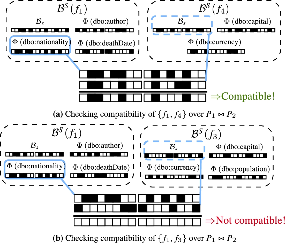
In order to prune fragments that do not contribute to the query result, as well as to determine subqueries that can be processed in parallel, Lothbrok builds a compatibility graph (Fig. 5), describing which of the relevant fragments are compatible for the given query, i.e., which fragments produce join results with one another for each join in the query. Specifically, two fragments are said to be compatible for a given query if the intersection of the corresponding SPBF partitions is non-empty, i.e., if the sets of entities represented by these partitions could have some common elements.
As an example, consider again the query Q and fragments from the running example in Fig. 4. In this case,
In other words, a compatibility graph is an undirected graph where nodes are the relevant fragments and edges describe the compatible ones. Structurally, a compatibility graph is thus defined as follows:
Definition 18
Definition 18(Compatibility Graph).
A compatibility graph
– F is a set of fragments
–
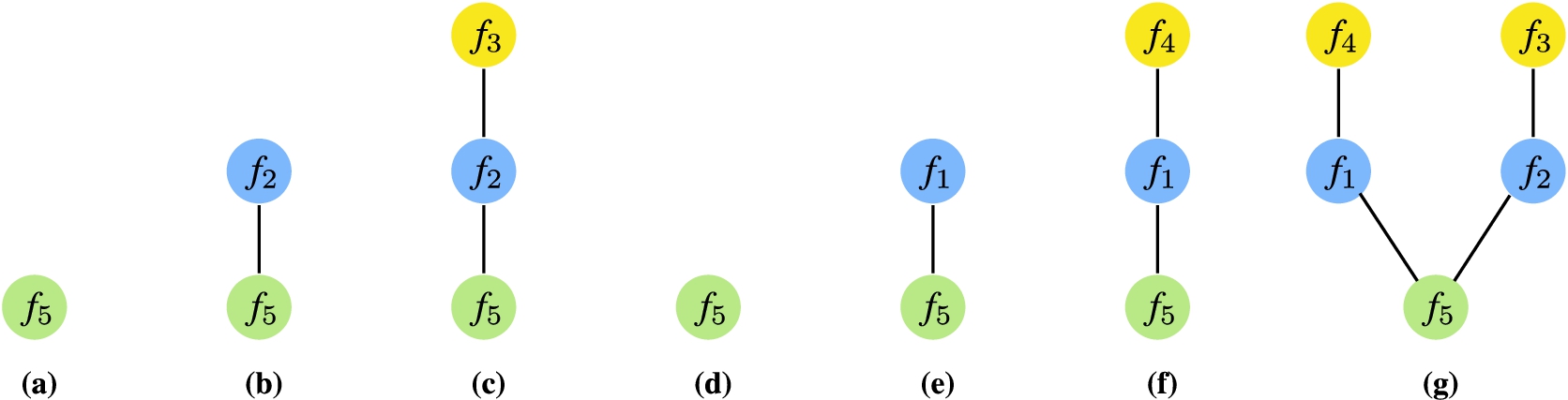
Consider again the running example in Fig. 4, and the example compatibility graph in Fig. 8(g). As we saw in Fig. 7,
Algorithm 1
Compute the compatibility graph of a BGP over an SPBF index
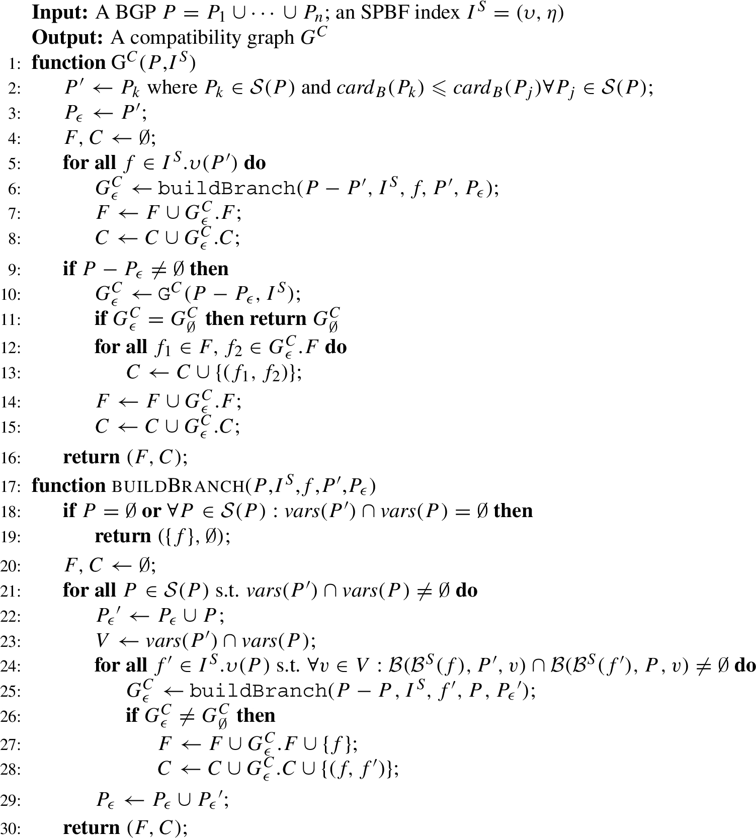
In the following, we detail how Algorithm 1 computes the compatibility graph by going through the algorithm showing a step-by-step example of how the compatibility graph is built in the running example in Fig. 4 (visualized in Fig. 8). Recall the function
Figure 8 shows how Algorithm 1 builds the compatibility graph for query Q in Fig. 4(a). In the following, we go through each intermediate step of the algorithm, describing the intermediate compatibility graphs built in the process. First, the
Then, the relevant fragments for the selected star pattern are found using the
The buildBranch
Instead, the for loop in lines 21–29 iterates through the star patterns
Fig. 8.
Recursively building the compatibility graph for the query in Fig. 4(a) by applying Algorithm 1 resulting in
Since
In the next iteration of the for loop in line 5, the buildBranch is called with
The if statement in lines 9–15 ensures that subqueries with star patterns that do not join (i.e., in the case of Cartesian products) are included in the compatibility graph. This is done by keeping track of the considered star patterns in P using the accumulator
The output of Algorithm 1 in the example is the compatibility graph shown in Fig. 8(g), specifying that
Algorithm 1 and the definition of SPBF indexes (Definition 15) ensure that pruned fragments do not contribute to the query result, i.e., that our pruning method does not miss any potential results. This follows from the theorem:
Theorem 1.
For any BGP P, SPBF index
A high-level sketch of the proof of Theorem 1 follows. Algorithm 1 only prunes fragments when the condition in line 24 is false. Furthermore, this condition is only false when the bitvectors for the two fragments do not overlap; if there is any kind of overlap, even on a single bit, the condition is true. If the two fragments contain a common value, then by definition this value is mapped to the same positions in the corresponding bitvectors, and they will overlap at least on those bits. Hence, Theorem 1 holds, and we do not miss any potential results.
5.2.Cardinality estimation
In Section 4.2 we have described how Lothbrok fragments knowledge graphs based on characteristic sets. Furthermore, in Section 4.3 we described how SPBF indexes connect the objects in a fragment to the predicates they occur in triples with. Since the SPBF of a fragment includes partitioned bitvectors describing the subjects and objects (Definition 15), we can estimate the number of values within these partitioned bitvectors and use those estimations to obtain cardinality estimations in a similar way as [52,55].
Table 1
Estimated cardinalities for the SPBFs
| Partitioned bitvector | Partitioned bitvector | ||
| 1000 | 100 | ||
| 5000 | 100 | ||
| 1000 | 150 | ||
| 1000 | 100 | ||
| 2000 | 200 | ||
| 3000 | 200 | ||
| 2000 | 500 | ||
| 0 | 100 | ||
| 50 | 0 | ||
| 8000 | 500 | ||
| 8000 | 1000 | ||
| 9000 |
Note that the cardinality estimation technique presented in this section is used by the Dynamic Programming (DP) algorithm (Section 5.3) to find the cheapest costing query execution plan including all the relevant fragments, and is not used to rank relevant fragments according to the cardinalities. Recall the
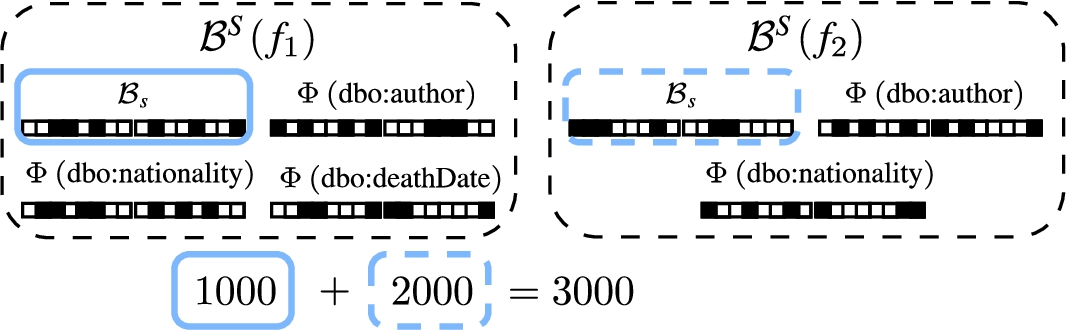
To estimate the cardinality of star-shaped subqueries, we utilize the fact that the subjects are described by a single partitioned bitvector. For a star-shaped subquery asking for the set of unique subject values described by a given set of predicates (i.e., queries with the DISTINCT keyword), the cardinality can be estimated as the sum of the number of subjects in each fragment that includes all the predicates in the star-shaped subquery. For instance, the cardinality of
Given a star pattern P and a fragment f, the cardinality of P over f, assuming that f is a relevant fragment for P, is the number of values in the partitioned bitvector on the subject position in
For queries not including the DISTINCT keyword, we need to account for duplicates by considering, on average, the number of triples for each non-variable predicate value in P that each subject value is associated with. Given a star pattern P and fragment f, let
Henceforth, we will refer to the more generalized function
Fig. 9.
Estimating the cardinality of
Consider, for instance, in the running example, the star-shaped BGP
Fig. 10.
Estimating the cardinality of
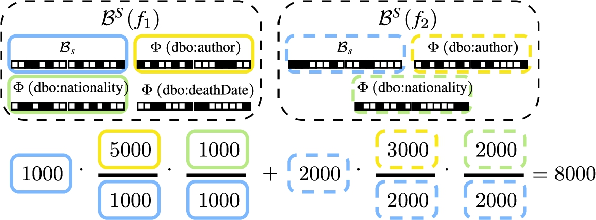
If, instead, the DISTINCT keyword was not included in the query, the cardinality
Until now, the cardinality estimations presented in this section are useful for estimating the cardinality of individual star patterns in a query [52,55]. However, to estimate the cardinality of arbitrary BGPs, [28] introduced characteristic pairs that describe the connections between IRIs described by different characteristic sets. In our case, however, we rely on the SPBFs of the relevant fragments to compute characteristic pairs without storing additional information; by intersecting the partitioned bitvectors on the positions corresponding to the join variable, we can estimate the selectivity of a given join and use that to estimate the cardinality of the join.
To achieve this, we first extend the framework for cardinality estimation described above to enable cardinality estimation of an entire query execution plan. This is straightforward for Cartesian products, unions, and selections; for Cartesian products it is the multiplication of the cardinality of the operands, for unions it is the sum of the cardinality of the operands, and for selections it is the cardinality of the star pattern over a specific fragment defined in Equations (4) and (5). Given the reasoning above, we define the cardinality of a query execution plan Π,
To compute the cardinality of any join
The function
Recall the
Fig. 11.
Estimating the cardinality of
![Estimating the cardinality of Π=([[P2]]f4n2⋈n2[[P1]]f1n2)∪([[P2]]f3n3⋈n3[[P1]]f2n3) with the DISTINCT keyword using the cardinalities from Table 1 and equation (9).](https://content.iospress.com:443/media/sw/2023/14-6/sw-14-6-sw233438/sw-14-sw233438-g012.jpg)
As an example, consider computing the cardinality
Fig. 12.
Estimating the cardinality of Π in Fig. 13(d) without the DISTINCT modifier for (a)
![Estimating the cardinality of Π in Fig. 13(d) without the DISTINCT modifier for (a) Π1=[[P2]]f4n2⋈n2[[P1]]f1n2 and (b) Π2=[[P2]]f3n3⋈n3[[P1]]f2n3. The output of equation (7) is thus the sum of the two formulas (625+225=850).](https://content.iospress.com:443/media/sw/2023/14-6/sw-14-6-sw233438/sw-14-sw233438-g013.jpg)
For queries without the DISTINCT keyword, we once again consider the average predicate occurences. However, since the predicate occurrences in Π are already considered in
Once again, computing the cardinality of Π in Fig. 13(d) not including the DISTINCT keyword is
5.3.Optimizing query execution plans
In the last step of the query optimizer (Fig. 5), Lothbrok builds an annotated query execution plan using a Dynamic Programming (DP) algorithm, that determines which parts of the query can be processed in parallel based on the compatibility graph (as explained in Section 5.1). Furthermore, the DP algorithm is locality-aware, meaning it finds the join delegations that minimize the number of intermediate results that have to be transferred between nodes when executing the plan, called the transfer cost.
To do this, the DP algorithm incrementally builds the plan for each subquery, by checking the transfer cost of the possible join combinations and delegations, and selects the cheapest one. In the remainder of this section, we will first define the cost function used by the DP algorithm, after which we will detail the DP algorithm itself.
Algorithm 2
Compute the transfer cost of a query execution plan
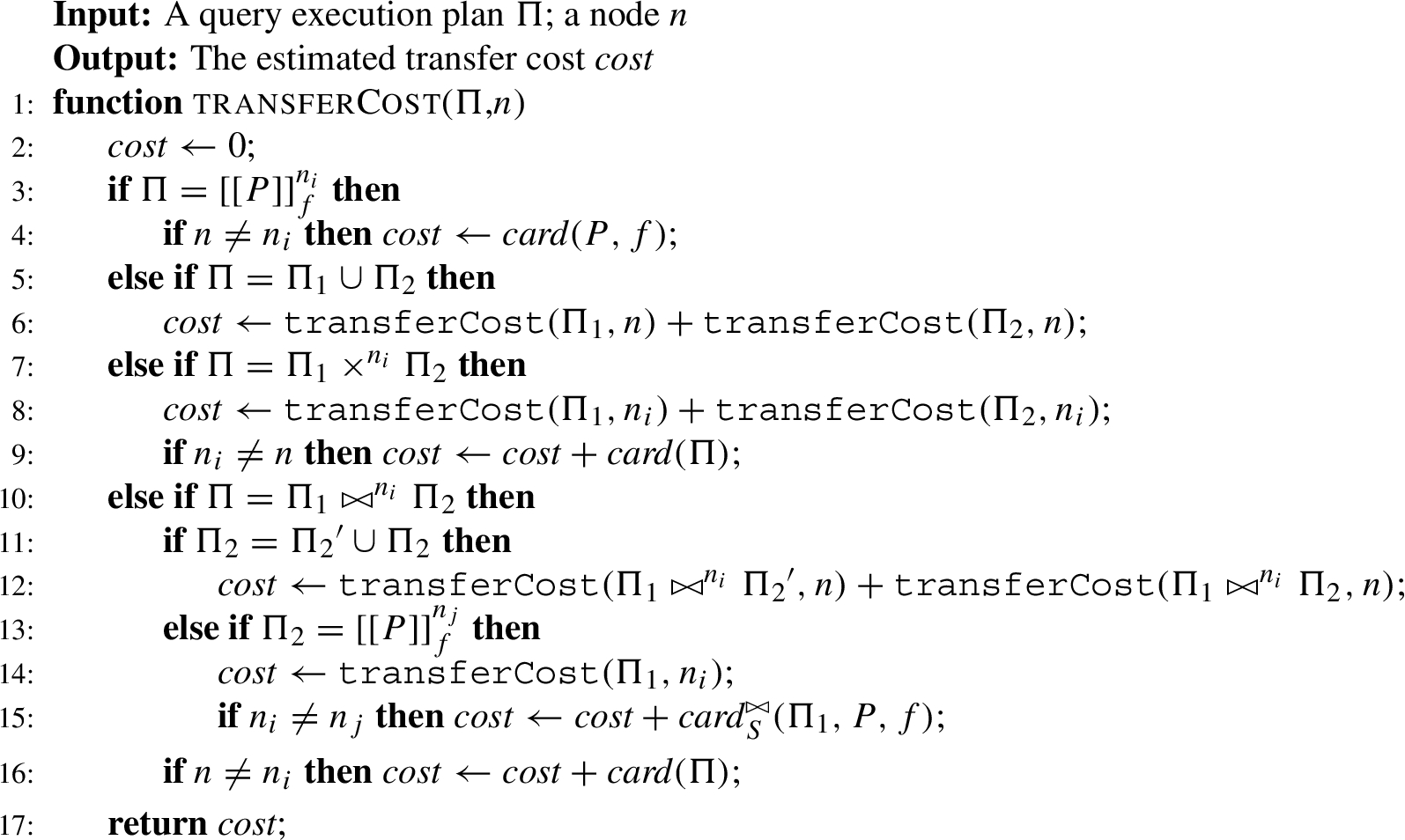
Using the cardinality estimation technique in Section 5.2, Algorithm 2 shows how the transfer cost of a query execution plan Π on a node n is computed taking into account the locality of the fragments. First, if
If, instead,
Otherwise, if
Finally, if
In addition to the transfer cost in Algorithm 2, we add the cardinality of the execution plan to the cost function used by the DP algorithm, since these results also have to be transferred to the user. The cost of processing a query execution plan Π over a node n is formally defined as follows.
Using the cost function in Equation (11), the DP algorithm finds the lowest costing execution plan by incrementally merging the cheapest (sub)plans for the smaller subqueries, and computing the cost of each possible join combination and delegation. Furthermore, to merge the subplans, the DP algorithm uses the compatibility graph computed in the second step (Fig. 5), to determine which parts of those plans can be joined in parallel.
Algorithm 3 shows how the DP table is appended with the lowest costing execution plan for a given (sub)BGP P, node n, and compatibility graph
Consider, in the running example, the situation where the appendDPTable function is called with the parameters
Since
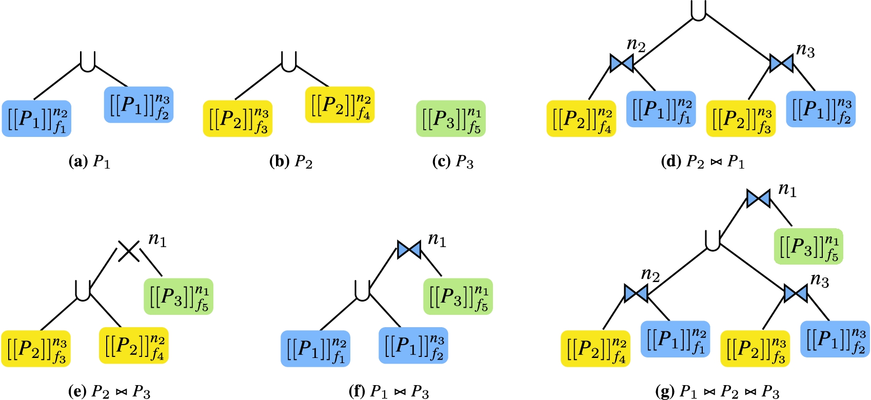
Table 2
Entries in the DP table for query Q (Fig. 4(a))
| Subquery | Execution plan | Cardinality | Cost |
| 8,000 | 8,000 | ||
| 650 | 650 | ||
| 9,000 | 9,000 | ||
| 850 | 1,700 | ||
| 5,850,000 | 5,850,650 | ||
| 1,688 | 9,688 | ||
| 154 | 1,004 |
Algorithm 3
Append DP table for a specific subquery
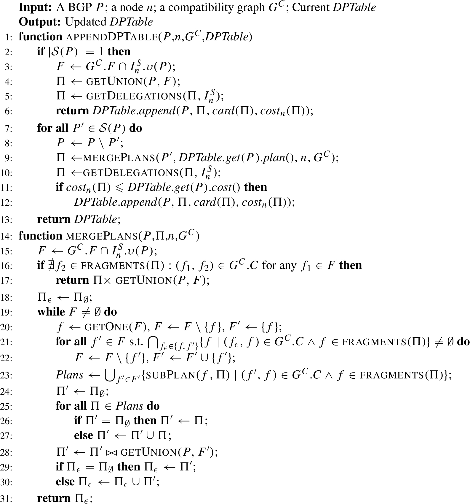
In the call to mergePlans in the first iteration of the for loop in lines 7–12, the function finds in line 15 the relevant fragments to
In the for loop in lines 21–22, the function determines, based on the edges in the compatibility graphs, which fragments in F that should be processed together, i.e., which fragments depend on some common fragments for the joining star patterns. In the above example, since
In line 23, we then determine the set of subplans in Π that the fragments in
Finally, the fragments in
Notice, that the function in lines 14–31 is called for each star pattern in the subquery, i.e., both
6.Query execution
Until now, we have described in Section 5 how Lothbrok obtains a query execution plan using compatibility graphs and locality information provided by the SPBF indexes. In this section, we detail the last step from Fig. 5, i.e., the Query Execution step, and thus how Lothbrok evaluates a query given a query execution plan.
Given a BGP P, a compatibility graph
Definition 19
Definition 19(Selector Function [3,6,32]).
Given a node n, a star pattern P, and a finite set of distinct solution mappings Ω, the star pattern-based selector function for P and Ω, denoted
In line with [3,6,32], and to avoid long-running requests on each node, we apply pagination to the results of star pattern requests, i.e., we group the results into reasonably sized pages to avoid excessive data transfer. The page size used in our experimental evaluation (Section 7) is the page size recommended by related work [3,6,32], i.e., 100. However, for ease of presentation, we assume that all results can fit into one page when presenting the approach to query processing. Furthermore, to avoid underestimating costs caused by the selector function returning some duplicate values (e.g., when the same subject has multiple object values for a specific predicate), our implementation always uses
Algorithm 4
Evaluate a join plan
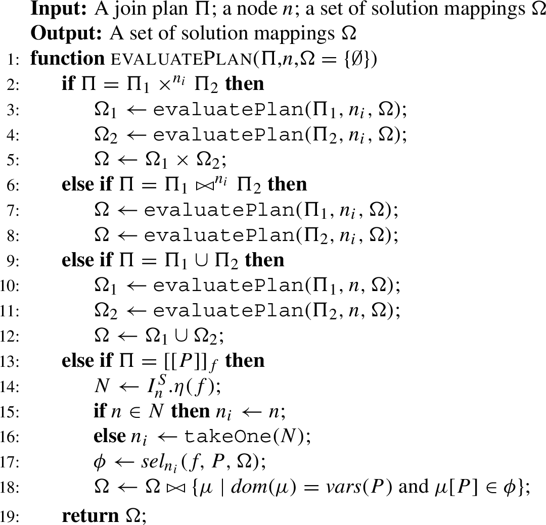
Let
Consider, for instance, the query execution plan Π shown in Fig. 13(g) for query Q in Fig. 4(a) processed by node
Since
When processing the plan
Fig. 14.
Processing Π in Fig. 13(g) on
![Processing Π in Fig. 13(g) on n1 by (a) delegating [[P2]]f4⋈n2[[P1]]f1 to n2 and [[P2]]f3⋈n3[[P1]]f2 to n3 concurrently and (b) processing the join between these 850 results and [[P3]]f5 locally on n1 to achieve the 154 results (solid arrows denote neighbors, dotted arrows subquery delegation, and dashed arrows transferring of intermediate results). n1 can send intermediate results to n3 since it is within its horizon.](https://content.iospress.com:443/media/sw/2023/14-6/sw-14-6-sw233438/sw-14-sw233438-g018.jpg)
Upon receiving the 500 results in line 7, Algorithm 4 makes another recursive call in line 8 to evaluatePlan on node
While
The 850 intermediate results in Ω found by processing
As mentioned above, our implementation uses pagination of the results meaning, for instance, when processing the subplan
7.Experimental evaluation
The experimental evaluation compares Lothbrok with two state-of-the-art approaches building on P2P systems: Piqnic [4] and ColChain [6] with the query optimization approach outlined in [5]. To do this, we implemented33 the fragmentation, indexing, and cardinality estimation approach as a separate package in Java 8 and modified Piqnic’s and ColChain’s query processors to use it. Like ColChain and Piqnic, Lothbrok’s query processor is implemented as an extension to Apache Jena.44 Fragments in our implementation are stored as HDT files [23], allowing for efficient processing of the star patterns. We provide all source code, experimental setup (queries, datasets, etc.), and the full experimental results on our website.55
7.1.Experimental setup
In this section, we detail the experimental setup, including a characterization of the used datasets and queries, the hardware and software setup, experimental configuration, as well as the evaluation metrics.
Datasets. We used two different benchmark suites for data in our experiments, LargeRDFBench [61] and WatDiv [9], with a total of four datasets, detailed in Table 3 along with some characteristics and statistics. LargeRDFBench is a well-known benchmark suite for federated RDF engines that comprises 13 different, interlinked datasets with over a billion triples in total, used to test Lothbrok in a realistic setting where users would upload several interlinked datasets to a network and ask queries with varying complexity. Notice that the total number of fragments over the datasets in LargeRDFBench exceed the number of fragments for LargeRDFBench overall. This is due to some fragments spanning multiple datasets, e.g., LinkedTCGA-M and LinkedTCGA-E span the exact same fragments. WatDiv is a synthetic benchmark used to test the scalability of the approaches when the network is under heavy load, and to assess the impact of the query pattern on performance and network usage. We generated three differently sized WatDiv datasets, from 10 million triples to 1 billion triples.
Table 3
Characteristics of the used datasets
| Dataset | #triples | #subjects | #predicates | #objects | #fragments | Struct. [21] |
| LargeRDFBench | 1,003,960,176 | 165,785,212 | 2,160 | 326,209,517 | 2,160 | 0.926 |
| LinkedTCGA-M | 415,030,327 | 83,006,609 | 6 | 166,106,744 | 8 | 1 |
| LinkedTCGA-E | 344,576,146 | 57,429,904 | 7 | 84,403,402 | 8 | 1 |
| LinkedTCGA-A | 35,329,868 | 5,782,962 | 383 | 8,329,393 | 209 | 0.98 |
| ChEBI | 4,772,706 | 50,477 | 28 | 772,138 | 21 | 0.34 |
| DBPedia-Subset | 42,849,609 | 9,495,865 | 1,063 | 13,620,028 | 1,774 | 0.196 |
| DrugBank | 517,023 | 19,693 | 119 | 276,142 | 11 | 0.726 |
| GeoNames | 107,950,085 | 7,479,714 | 26 | 35,799,392 | 23 | 0.518 |
| Jamendo | 1,049,647 | 335,925 | 26 | 440,686 | 7 | 0.961 |
| KEGG | 1,090,830 | 34,260 | 21 | 939,258 | 3 | 0.919 |
| LinkedMDB | 6,147,996 | 694,400 | 222 | 2,052,959 | 135 | 0.729 |
| NYT | 335,198 | 21,666 | 36 | 191,538 | 6 | 0.731 |
| SWDF | 103,595 | 11,974 | 118 | 37,547 | 12 | 0.426 |
| Affymetrix | 44,207,146 | 1,421,763 | 105 | 13,240,270 | 12 | 0.506 |
| watdiv10M | 10,916,457 | 521,585 | 86 | 1,005,832 | 86 | 0.42 |
| watdiv100M | 108,997,714 | 5,212,385 | 86 | 9,753,266 | 86 | 0.42 |
| watdiv1000M | 1,092,155,948 | 52,120,385 | 86 | 92,220,397 | 86 | 0.42 |
Fig. 15.
Characteristics of the computed fragments over all the included datasets.
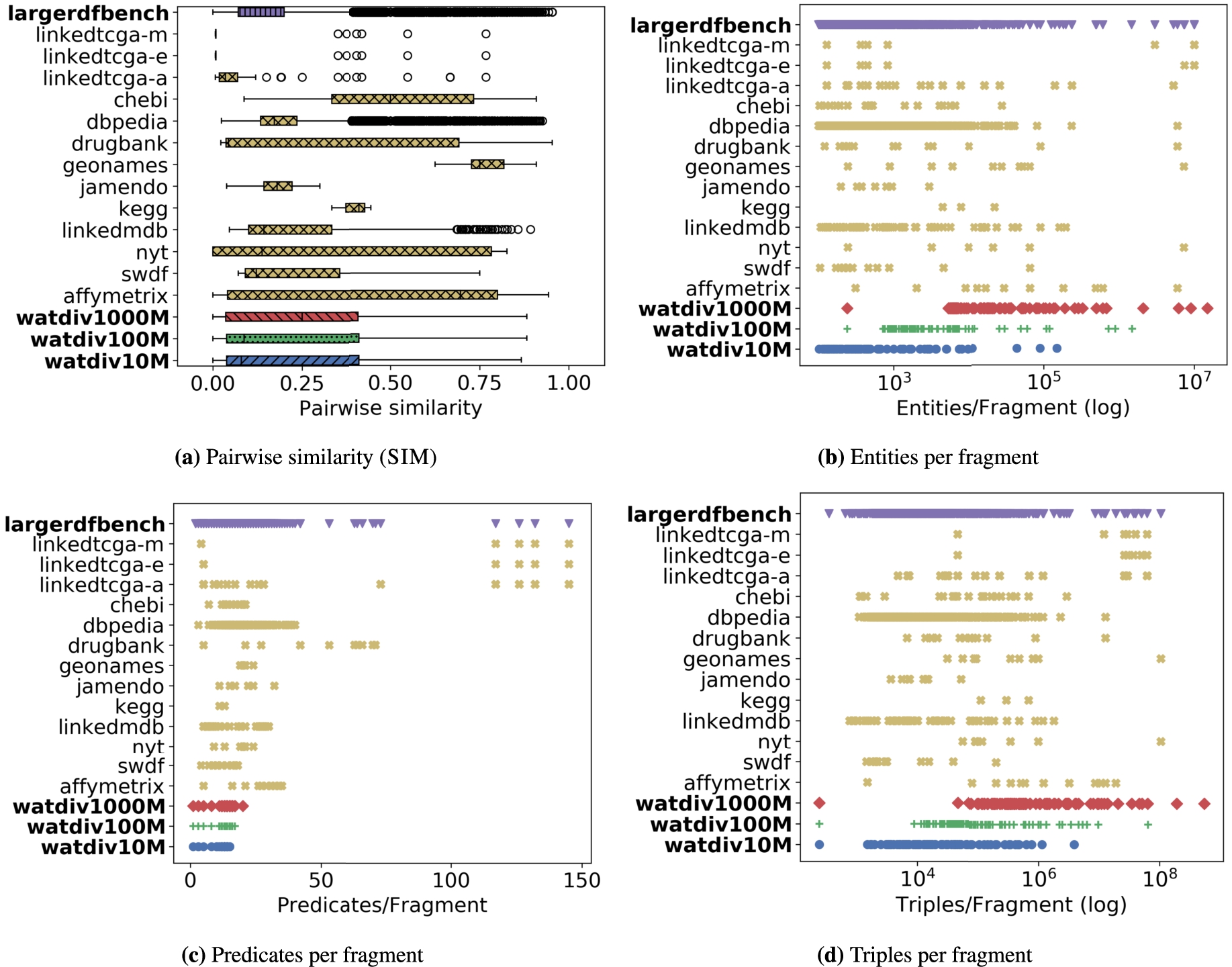
Fragments. To provide a fair comparison between the systems with and without Lothbrok, we created an equal number of fragments for both fragmentation methods, characteristic sets (Section 4.2) and predicate-based, following the approach outlined in Section 4.2. Fig. 15 shows an overview of the following characteristics of each fragment over each dataset: pairwise similarity SIM (Fig. 15(a)): given two fragments
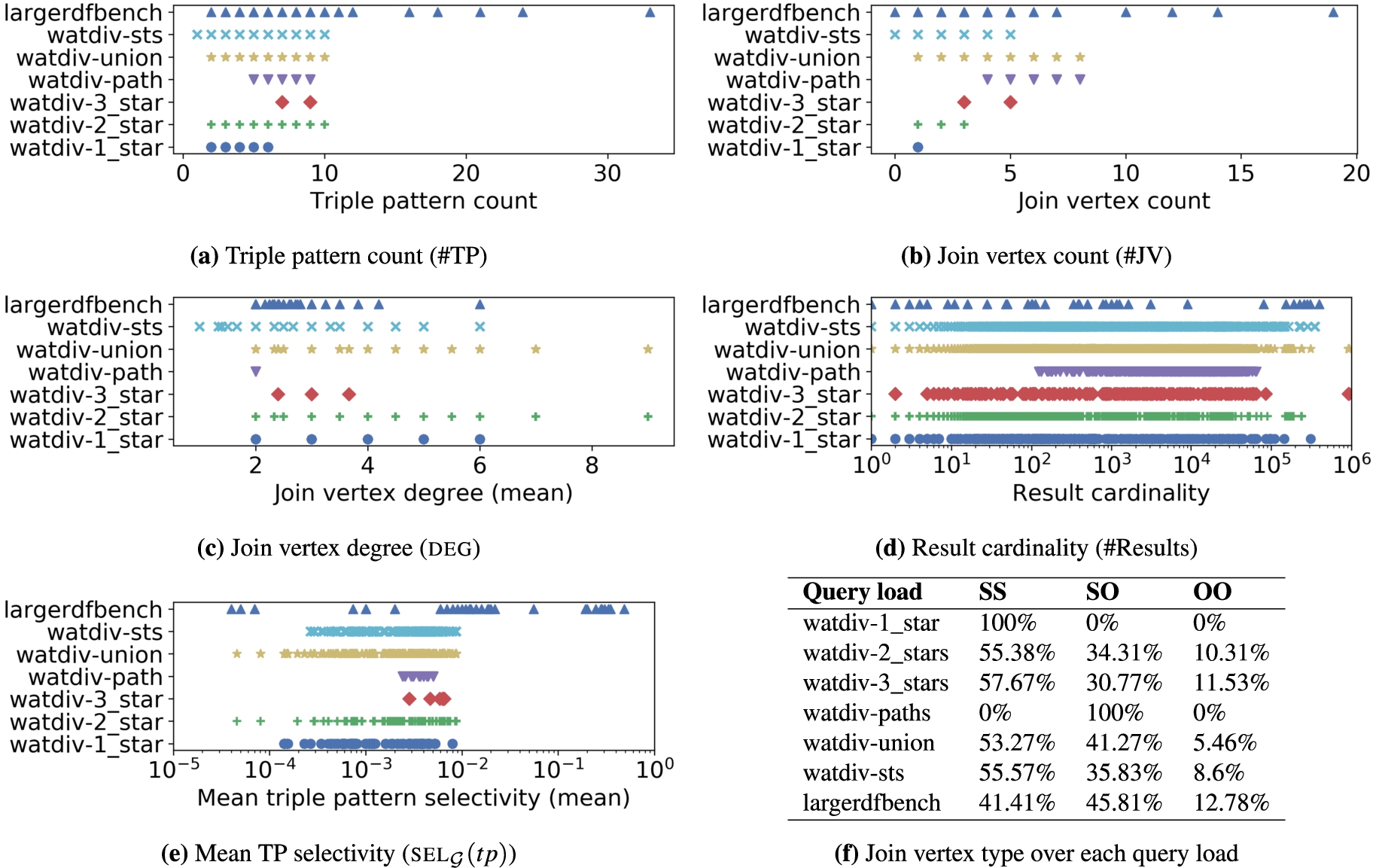
Queries. LargeRDFBench includes 40 queries [61] in five different categories of varying complexity: Simple (S), Complex (C), Large Data (L), and Complex and High Data Sources (CH). For WatDiv, we used WatDiv star query loads from [3] consisting of 1–3 star patterns, called the watdiv-1_star, watdiv-2_star, and watdiv-3_star query loads, as well as a query load consisting of path queries, i.e., queries where each star pattern only has one triple pattern, called the watdiv_path query load. Each of these query loads consists of 6,400 different queries. Furthermore, we combine the aforementioned query loads into a single query load called watdiv-union. Last, we created a query load with 19,968 queries from the WatDiv stress testing query templates (156 per node) called watdiv-sts. The complete set of queries is available on our website5.
Fig. 16 shows an overview of the following characteristics of each load [3,10]: Triple pattern count #TP (Fig. 16(a)), join vertex count #JV (Fig. 16(b)), join vertex degree deg (Fig. 16(c)), result cardinality #Results (Fig. 16(d)), mean triple pattern selectivity sel
Experimental Configuration. We compare the following systems: (1) Piqnic [4] using PPBF indexes [5] (Piqnic), (2) Lothbrok on top of Piqnic (Lothbrok
Fig. 16.
Characteristics of all query loads (WatDiv query loads over watdiv100M; statistics over the watdiv10M and watdiv1000M datasets can be found on our website
Hardware Configuration. For all configurations and P2P systems, we ran 128 nodes concurrently on a virtual machine (VM) with 128 vCPU cores with a clock speed of 2.5 GHz, 64KB L1 cache, 512KB L2 cache, 8192KB L3, and a total of 2TB main memory. To spread out resources evenly across nodes, all nodes were restricted to use 1 vCPU core and 15GB memory, enforced using the -Xmx and -XX:ActiveProcessorCount options for the JVM. Furthermore, to simulate a more realistic scenario, where nodes are not run on the same machine, we simulated a connection speed of 20 MB/s.
Evaluation Metrics. We measured the following metrics:
– Workload Time (WT): The amount of time (in milliseconds) it takes to complete an entire workload including queries that time out.
– Throughput (TP): The number of completed queries in the workload divided by the total workload time (i.e., number of queries per minute).
– Number of Timeouts (NTO): The number of queries that timed out (timeout being 1200 seconds).
– Query Execution Time (QET): The amount of time (in milliseconds) elapsed between when a query is issued and when its processing has finished.
– Query Response Time (QRT): The amount of time (in milliseconds) elapsed between when a query is issued and when the first result is computed.
– Query Optimization Time (QOT): The amount of time (in miliseconds) elapsed between when a query is issued and when the optimizer has finished (i.e., when query execution starts).
– Number of Requests (REQ): The number of requests made between nodes when processing a query (including requests made from nodes that have been delegated subqueries).
– Number of Transferred Bytes (NTB): The amount of data (in bytes) transferred between nodes when processing a query (including data transferred to and from nodes that have been delegated subqueries).
– Number of Relevant Nodes (NRN): The number of distinct nodes that replicate fragments containing relevant data to a query.
– Number of Relevant Fragments (NRF): The number of distinct fragments containing relevant data to a query.
Software Configuration. Unless otherwise specified, we used the following parameters when running the systems. For ColChain, we used the following parameters recommended in [6]: Community Size: 20, Number of Communities: 200. For Piqnic, we use the following parameters recommended in [4]: Time-to-Live (number of hops): 5, Number of Neighbors: 5. The replication factor for Piqnic (i.e., the percentage of nodes replicating each fragment) was matched with the size of the communities in ColChain to provide a better comparison. Nodes were randomly assigned neighbors throughout the network. The page size (i.e., how many results can be returned with each request, was set to 100. Furthermore, to limit the size of HTTP requests, the number of results that each system was allowed to attach to each request (i.e.,
Fig. 17.
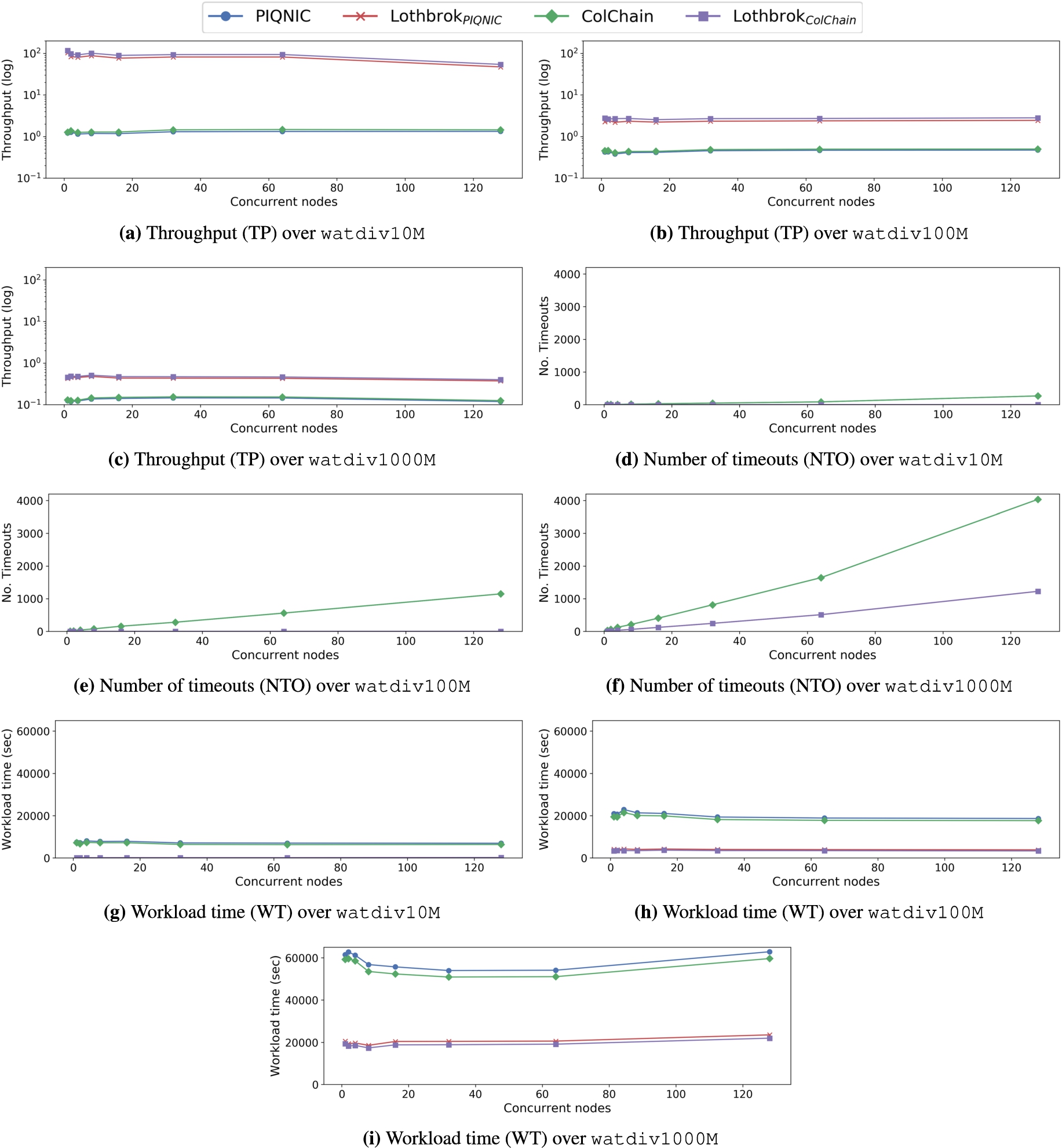
Throughput (TP), number of timeouts (NTO), and workload time (WT) for watdiv-sts over the watdiv10M, watdiv100M, and watdiv1000M datasets.
7.2.Scalability under load
In these experiments, we ran the watdiv-sts queries over each WatDiv dataset in configurations where
Figures 17(d)–17(f) show the number of queries that timed out (TO) of the watdiv-sts query load over each configuration for each WatDiv dataset. As expected, the number of timeouts increases relatively linearly with the number of nodes issuing queries concurrently. This is due to the fact that when more nodes issue queries, more queries in total are executed, meaning the total number of the queries that time out increases. Generally, the queries that time out correspond to query templates that result in a large number of intermediate results, e.g., by using the rdfs:label predicate. Furthermore, Piqnic and ColChain incur significantly more timeouts without Lothbrok compared to with Lothbrok. In fact, for both watdiv10M and watdiv100M, Lothbrok experiences no timeouts while Piqnic and ColChain experience 267 timeouts for watdiv10M and 1,148 timeouts for watdiv1000M. Even for watdiv1000M, the number of timeouts experienced by Lothbrok is just 1,151 while Piqnic and ColChain both experience 4,036 timeouts. Furthermore, Piqnic and ColChain incur the exact same number of timeouts.
While queries can time out for several different reason, the queries that timed out in our experiments have some common characteristics. Specifically, they are typically the queries that result in a large number of intermediate results. This is particularly the case for Piqnic and ColChain, since general predicates such as rdf:type result in querying large fragments and many intermediate results. Lothbrok is able to mitigate this effect by processing those triple patterns as part of a larger star pattern, lowering the total number of intermediate results. On the other hand, the few queries that timeout for Lothbrok over watdiv1000M are the queries specifically with a large number of star patterns with very common characteristic sets as we see in Section 7.3. A deeper analysis of what causes systems like Piqnic and ColChain to timeout requires further research that is out of scope for this paper; nevertheless, it is an interesting aspect to look into in the future.
Figures 17(g)–17(i) show the workload time (WT) for each configuration. In line with the throughput and number of timeouts, Lothbrok incurs a significantly lower average workload time than Piqnic and ColChain across all experiments and datasets. The slight decrease in the workload time for fewer nodes can be attributed to the network being able to process more queries concurrently when the overall load is relatively low. Nevertheless, the average workload time only increases slightly even when all nodes issue queries concurrently.
Overall, our experimental results show that, even when the network is under heavy query processing load, Lothbrok increases the query throughput and decreases the average workload time significantly compared to state-of-the-art decentralized systems. In fact, the increase in performance is up to two orders of magnitude. As a result, Lothbrok is also able to finish more queries without timing out.
7.3.Impact of query pattern
To test the impact of the query pattern on the performance of Lothbrok, we ran the watdiv-1_star, watdiv-2_star, watdiv-3_star, watdiv-path, watdiv-union, and watdiv-sts query loads on each system; the watdiv-sts queries consist of, on average, more selective star patterns compared to the other WatDiv query loads (Fig. 16).
Fig. 18.
Query execution time (QET) and query response time (QRT) for the WatDiv datasets.
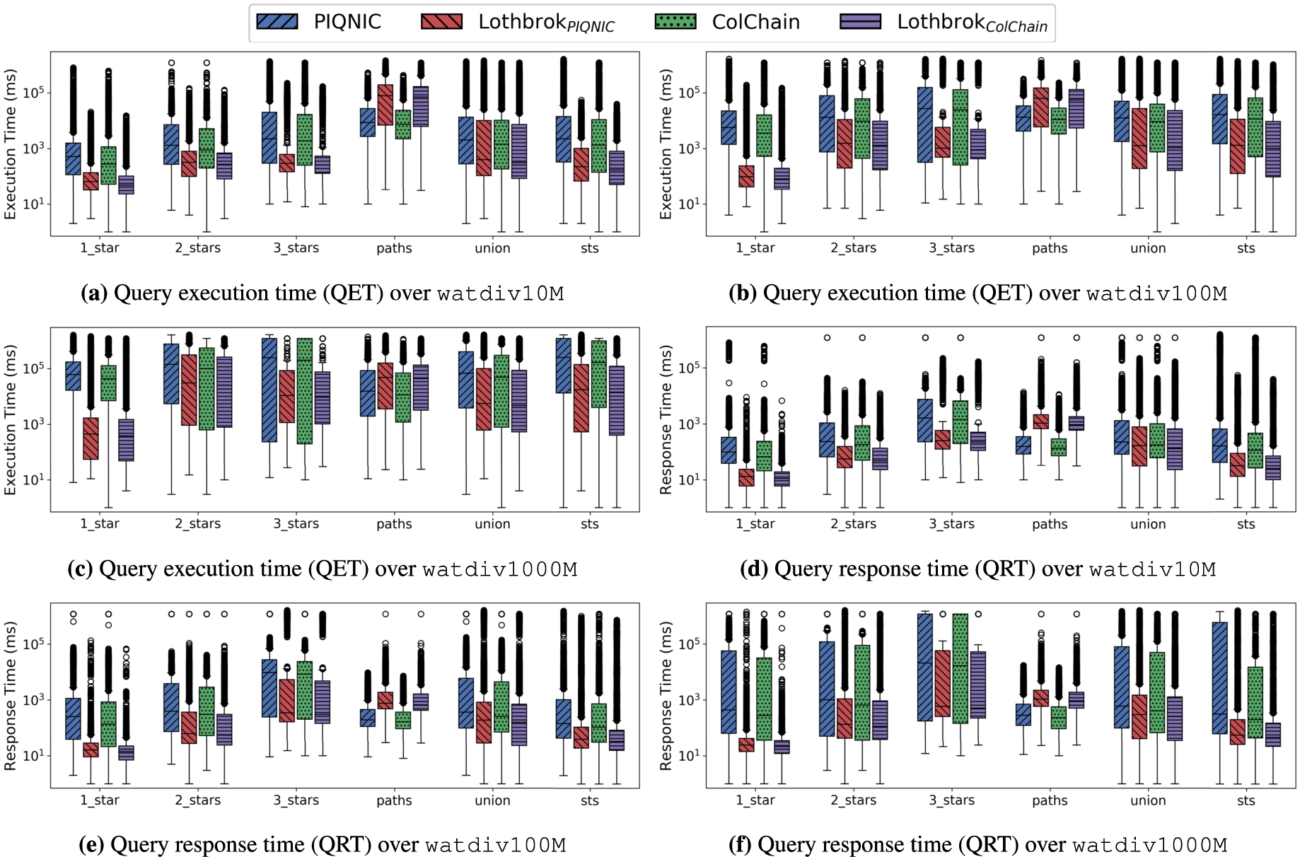
Figures 18(a)–18(c) show the execution time (QET) for each WatDiv query load over each WatDiv dataset, and Figs 18(d)–18(f) show the response time (QRT) for each WatDiv query load in logarithmic scale. Our results show that Lothbrok has significantly better performance across all datasets for almost every query load. As expected, the improvement in performance is more significant for the query loads with a lower number of star patterns. This is due to the fact that since the star patterns within these queries represent a large part of the query, Lothbrok has to issue fewer requests overall, lowering the network overhead. For instance, the queries in the watdiv-1_star query load can by Lothbrok be answered by issuing 0.89 requests per 90 results66, whereas Piqnic and ColChain have to issue 9.27 requests per 90 results on average, for watdiv1000M in our experiments. In the watdiv-3_star query load, the improvement in performance is more modest across the datasets since each star pattern is a relatively small part of the query resulting in a higher number of requests; however, on average, we still see a performance increase of up to an order of magnitude.
Fig. 19.
Number of relevant fragments (NRF) and number of relevant nodes (NRN) for the WatDiv datasets.
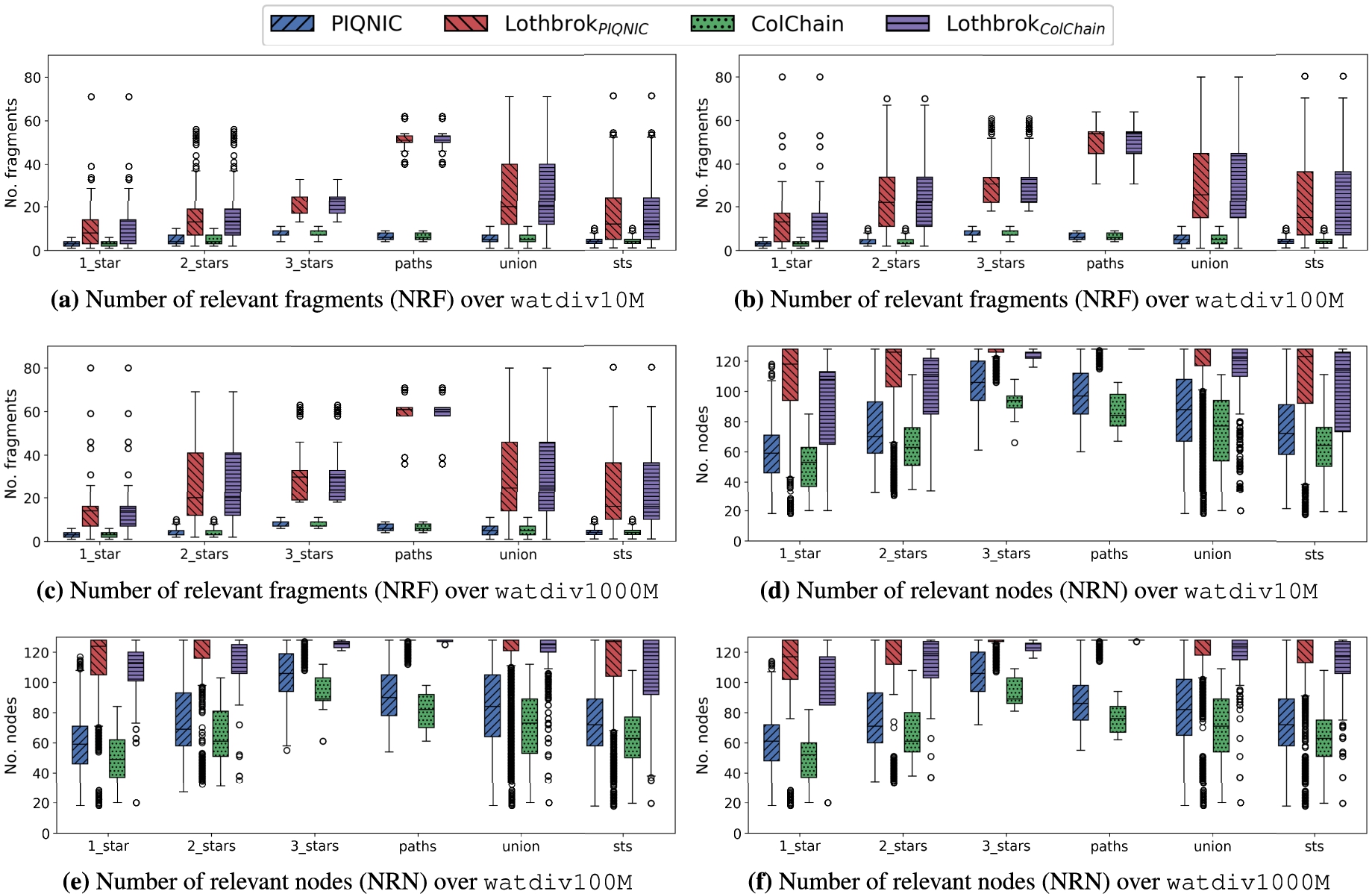
We notice that for the watdiv-path query load, Lothbrok actually has a slightly worse performance both in terms of QET and QRT compared to Piqnic and ColChain due to higher network usage. Fig. 19 shows the number of relevant fragments (NRF) and the number of relevant nodes (NRN) for each query load over each dataset after optimization (similar figures are provided for NRF and NRN before optimization on our website5). Analyzing these results, we see that the decreased performance for watdiv-path is caused by Lothbrok having a significantly larger number of relevant fragments and by extension a larger number of relevant nodes compared to Piqnic and ColChain. In fact, this is the case for all the WatDiv query loads (9 times larger for watdiv-path while up to 5 times larger for the other query loads); however, for the other query loads, this is compensated by the increased performance that the query optimization approach provides. This analysis is corroborated by the number of fragments pruned during optimization for each query load (figures provided on our website5); the watdiv-path query load has significantly less pruned fragments compared to the other query loads except watdiv-1_star. For Piqnic and ColChain, the number of relevant fragments will always equal the number of unique predicates in the query since one fragment is created per predicate; however, due to fragmenting the data based on characteristic sets, Lothbrok can encounter multiple fragments for each unique predicate in the query. Furthermore, the number of relevant fragments is, on average, more than twice as high for Lothbrok over the watdiv-path query load than over the other query loads. This is because the queries in this query load include between 5 and 9 star-shaped subqueries, each of which consists of a single triple pattern which is considerably less selective of characteristic set fragments than subqueries with more triple patterns (Fig. 16).
Nevertheless, the slightly worse performance for Lothbrok over watdiv-path is compensated by the significantly improved performance over the other query loads, so we still see a performance increase for the watdiv-union query load. As such, our experimental results show that Lothbrok is generally able to increase performance over queries with star-shaped subqueries (i.e., all other queries than path queries) significantly and that the increase in performance depends on the shape of the query; queries with fewer but larger star patterns (cf. Fig. 16(c)) show a bigger performance increase than queries with many but small star patterns.
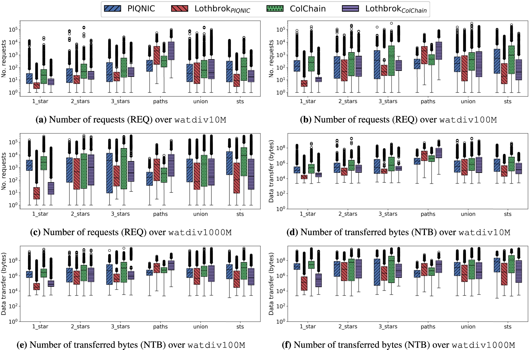
Fig. 20.
Number of requests (REQ) and number of transferred bytes (NTB) for the WatDiv datasets.
7.4.Network usage
Fig. 20 shows the network usage when processing WatDiv queries over each WatDiv dataset in terms of the number of requests (Figs 20(a)–20(c)) and the number of transferred bytes (Figs 20(d)–20(f)) in logarithmic scale. Lothbrok incurs a significant lower network overhead for all query loads except watdiv-path despite the larger number of relevant fragments as discussed in Section 7.3. This is caused by Lothbrok having to send significantly fewer requests for each star pattern since a star pattern can be processed entirely over the relevant fragments, even if there are more fragments (and thus nodes) to send the requests to. Again, the query loads with a smaller number of star patterns see a larger decrease in network usage since larger parts of the queries can be processed by individual nodes. Since the queries in the watdiv-path query load do not benefit from the star pattern-based query processing, the network usage is slightly higher; however, even still, the watdiv-union shows an improvement in the network usage for Lothbrok. These results are in line with the experiments shown in Sections 7.2 and 7.3 and support the hypothesis that Lothbrok increases performance by lowering the network overhead when processing queries, compared to state-of-the-art systems such as Piqnic and ColChain.
7.5.Performance of individual queries
In these experiments, we ran the LargeRDFBench queries three times on each system sequentially to test the performance of those individual queries and report the average results. Figure 21 shows the execution time (Fig. 21(a)), response time (Fig. 21(b)), and optimization time (Fig. 21(c)) for the C query load over LargeRDFBench in logarithmic scale. Similar figures for the other LargeRDFBench query loads are provided on our website5. The results in Fig. 21 are similar to the remaining query loads; we show the C query load since this query load had the most diversity in the performance across the queries.
Fig. 21.
Query execution time (a), response time (b), and optimization time (c) for the C query load over LargeRDFBench.
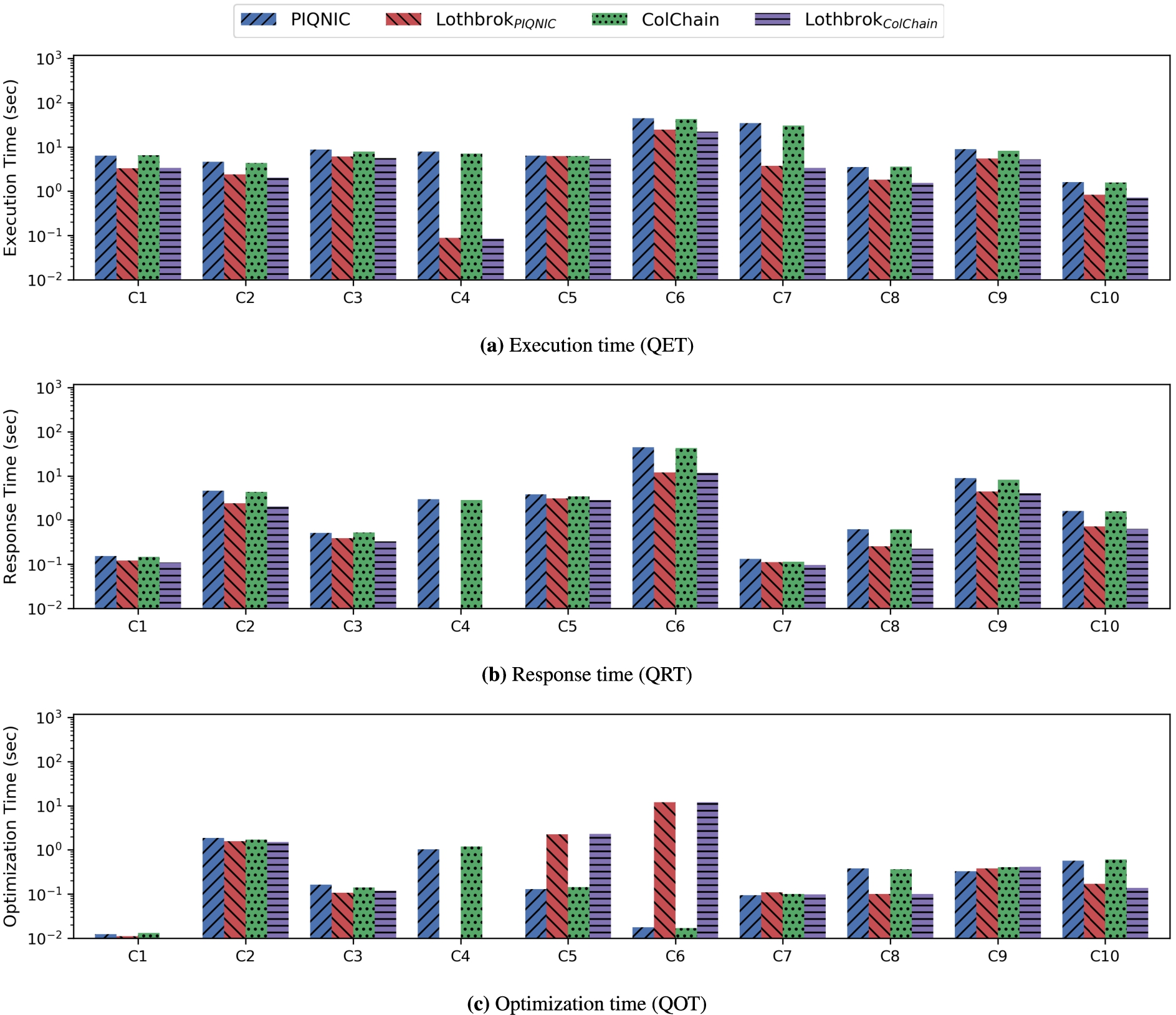
While, in our experiments, Lothbrok provides an improvement for the execution time (Fig. 21(a)) across all the queries in LargeRDFBench, the improvement varies based on the query shape in line with the findings of [3,13] and the query shape experiments shown in Section 7.3. For instance, query C4 consists of one highly selective star pattern with 6 unique predicates. Lothbrok is thus able to answer C4 with one request to the only fragment with that predicate combination, while Piqnic and ColChain have to send at least one request per triple pattern. Hence, Lothbrok has around two orders of magnitude better performance for this particular query. On the other hand, query C5 consists of four star patterns, two of which contain only one triple pattern with one of them being the very common rdfs:label predicate. As a result, Lothbrok has more than twice the number of relevant fragments for C5 compared to both Piqnic and ColChain. Nevertheless, Lothbrok still has slightly improved performance for C5 compared to Piqnic and ColChain since the query still contains two star patterns with three triple patterns each, meaning the increased optimization and communication overhead that the additional relevant fragments entail is offset by the benefits of processing the star patterns over the individual fragments. The response times (Fig. 21(b)) show a similar comparison between the systems as the execution times (Fig. 21(a)) with the exception of query C4. Again, the reason being that Lothbrok can process this query with a single request, and therefore the first result is obtained immediately after receiving the response to the request.
However, the optimization times (Fig. 21(c)) differ quite significantly depending on the number of relevant fragments to the query. For instance, queries like C5 and C6 (that contain a star pattern consisting of a single triple pattern with a very common predicate) incur a significant number of relevant fragments for Lothbrok (286 for C5 and 144 for C6) and thus a higher optimization time. This is the case, since a higher number of relevant fragments means a higher number of SPBFs have to be intersected which represents an overhead. In all of these cases, however, the benefits of processing entire star patterns over the fragments, in terms of decreased network overhead mean that the overall execution time is still lower for Lothbrok. This is especially the case for C6, which contains a star pattern with 6 triple patterns that in Piqnic and ColChain have to be processed individually. On the other hand, queries like C4 that contain few very selective star patterns have a low optimization time for Lothbrok, since each star pattern have very few relevant fragments. In the case of C4, Piqnic and ColChain have a relatively high number of relevant fragments due to one of the predicates being the common owl:sameAs predicate that occurs in multiple datasets. As a result, Piqnic and ColChain have a significantly higher optimization time for this query compared to Lothbrok.
Fig. 22.
Number of transferred bytes (NTB) (a), number of requests (REQ) (b), number of relevant fragments (NRF) (c), and number of relevant nodes (NRN) (d) for each LargeRDFBench query load.
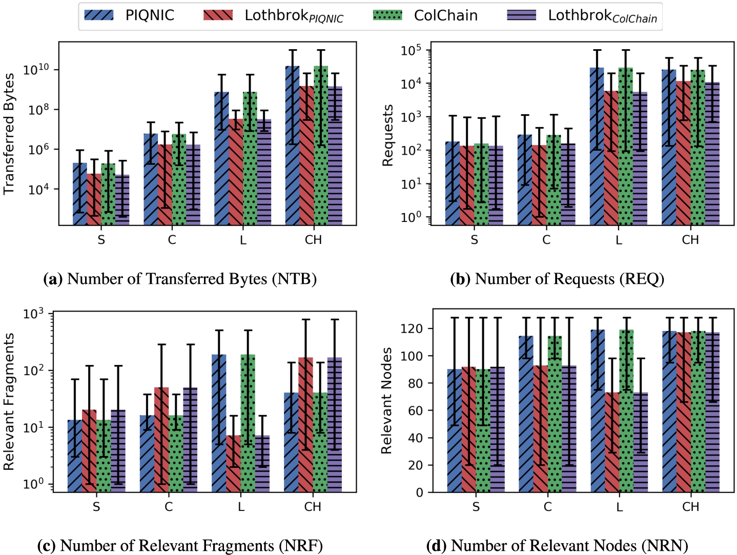
Figure 22 shows the number of transferred bytes (Fig. 22(a)), the number of requests (Fig. 22(b)), the number of relevant fragments (Fig. 22(c)), and the number of relevant nodes (Fig. 22(d)) for each LargeRDFBench query load in logarithmic scale. We provide figures displaying each measure in Fig. 22 for each individual LargeRDFBench query on our website5. As with the experiments shown in Section 7.4, Lothbrok clearly incurs a lower network usage than both Piqnic and ColChain, both in terms of data transfer (Fig. 22(a)) and the number of requests made (Fig. 22(b)). This, together with the performance experiments, shows that Lothbrok is able to reduce the network overhead significantly across all query loads and, in doing so, increase the performance overall.
Interestingly, while for most query loads, Lothbrok has a higher number of relevant fragments (Fig. 22(c)) in line with the experiments presented in Section 7.3, for the L query load, Lothbrok has a lower number of relevant fragments in most queries. The reason is that the queries in this query load mostly use data from the quite structured linkedTCGA datasets which contain few similar characteristic sets, thus incurring a low number of relevant fragments per star pattern. On the other hand, for Piqnic and ColChain, the fact that some star patterns with a low number of triple patterns include common predicates like rdf:type increases the number of relevant fragments. The number of relevant nodes (Fig. 22(d)) shows a similar trend to the number of relevant fragments since each fragment is replicated across 20 nodes; in some cases, however, where two relevant fragments are simultaneously replicated by some of the same nodes, the actual number of relevant nodes will be a bit lower than when the relevant nodes replicate exactly one relevant fragment.
Our results are similar for all query loads (figures provided on our website5) and show that even for the complex queries in query loads C and CH and the queries with a large number of intermediate results in query load L, Lothbrok presents a significant performance increase because it lowers the communication overhead. For some queries, this is quite significant; for instance the queries C4 and S3 where Lothbrok increases execution time by up to two orders of magnitude. Furthermore, some queries in the L and CH groups that timed out for Piqnic and ColChain, such as L3 and CH2, finished within the timeout of 1200 seconds for Lothbrok. This is in line with the results presented in Section 7.2 and suggests that Lothbrok is able to complete more queries within the timeout than the state-of-the-art systems.
7.6.Discussion
Our experimental evaluations show that Lothbrok significantly improves query performance while lowering the communication overhead compared to Piqnic and ColChain. Lothbrok does so by distributing subqueries to other nodes such that the estimated network cost is limited as much as possible, and by processing entire star patterns over the individual fragments. In doing so, Lothbrok decreases the network usage both in terms of the data transfer and number of requests, and increases performance by up to two orders of magnitude compared to the state of the art. Moreover, Lothbrok does so while providing scalable performance under load; in fact, even when all nodes in the network issue queries concurrently, Lothbrok maintains efficient query processing.
The only exception to the improved scalability and performance in our experiments is the slightly worse performance for path queries in Lothbrok compared to existing approaches. This is mainly caused by factors like similarity and coplanarity of fragments having an effect on the performance of Lothbrok that is not mitigated by star-shaped query optimizations. Specifically, we see an increased number of relevant fragments and lower number of pruned fragments per query incurred by Lothbrok over the path queries caused by many of the fragments containing very similar characteristic sets. Optimizing queries for such path queries is a difficult problem, corroborated by several previous studies [3,13,28,52,55], and was out of scope of this paper. Nevertheless, looking into query optimization for path queries is an interesting topic for future work. For instance, one possible solution to the path query optimization problem could be co-location of fragments relevant for common paths on the same nodes, similar to workload-aware fragmentation techniques [8,39], or storing and using statistics about commonly used paths as part of the query optimization step.
We emphasize that our goal with this work was not to beat client-server systems like SPF [3] or WiseKG [13] in terms of performance, rather we aimed at making query processing in the decentralized setup, where node failures can be tolerated [4], more feasible with high scalability. While this paper specifically aims to optimize queries, the nature of P2P networks means that processing queries comes at a performance cost due to queries having to be split across multiple nodes that is impossible to remove completely. In any case, P2P systems also have the benefit that the query processing effort is divided across several nodes. As such, even when the network incurs heavy load, the performance should stay relatively stable in contrast to the centralized solutions. In fact, our scalability experiments in Section 7.2 clearly support this since they show that the query throughput hardly decreases, even when all the nodes in the network process queries at the same time (Fig. 17). On the other hand, the analysis provided by [4,13] of SPF and WiseKG (both are client-server systems where all queries have to be evaluated on a single server holding all the data) show a significant decrease in query throughput when the load increases.
8.Conclusions
In this paper, we proposed Lothbrok, a novel query optimization approach for SPARQL queries over decentralized knowledge graphs. Lothbrok builds upon recent work on decentralized Peer-to-Peer (P2P) systems [4,6] and introduces a novel fragmentation technique based on characteristic sets [55], i.e., predicate families, as well as a novel indexing scheme that summarizes the sets of subjects and objects in a fragment using partitioned bitvectors. Furthermore, Lothbrok proposes a query optimization strategy based on cardinality estimation, fragment compatibility, and data locality that is able to delegate the processing of (sub)queries to other, neighboring nodes in the network that hold relevant data. We implemented our approach on top of two recent systems and evaluated Lothbrok’s capabilities over well-known benchmarking suites containing real-world data and queries, as well as the performance of Lothbrok under load using large-scale synthetic datasets and stress-testing query templates. The experimental results show that Lothbrok significantly reduces the network overhead when processing queries in a P2P network and, in doing so, increases performance by up to two orders of magnitude.
While Lothbrok generally improves performance, our experimental results showed that path queries have slightly worse performance for Lothbrok than existing approaches. As such, our future work includes looking into the optimization problem for path queries, e.g., by co-locating relevant fragments for common path patterns on the same nodes, similar to workload-aware partitioning techniques [8,39]. Furthermore, a complete analysis of the effects of graph complexity metrics, like density and centrality, on the fragment skew, query performance, and indexing strategy, as well as an analysis of different fragmentation techniques, e.g., based on SHACL/ShEx shapes [59,60], is important future work. We also plan to expand the range of supported queries to include aggregation and analytical queries [25,41], and add support for provenance both for data [11,29,31], so that the system has information about the origin of the data it uses, as well as for queries [35] so that the system can explain how query answers were computed. Finally, we plan to generalize our approach to other types of distributed graphs, extend the query optimizer to support relevance scores or benefit-based source selection [38], extend our approach with methods for handling inconsistent or conflicting data, analyze the benefits and tradeoffs of the merging procedure presented in Section 4 and indexes presented in Section 4.3 using even more diverse real-world datasets, and investigate the potential benefits of allowing execution plans of any shape (i.e., removing the assumption, given in Section 5, that execution plans are always left-deep).
Notes
1 ⊕ is defined in [5,6] as
2 As defined in https://www.w3.org/TR/rdf11-concepts/#vocabularies.
3 Code is available on the following GitHub repository: https://github.com/dkw-aau/Lothbrok-Java.
6 Even though one request can fetch up to 90 results, the average number of requests is lower than 1 since the nodes store some data locally.
Acknowledgements
This research was partially funded by the Independent Research Fund Denmark (DFF) under grant agreement no. DFF-8048-00051B and the Poul Due Jensen Foundation.
References
[1] | M. Acosta and M. Vidal, Networks of linked data eddies: An adaptive web query processing engine for RDF data, in: The Semantic Web – ISWC 2015 – 14th International Semantic Web Conference, Proceedings, Part I Bethlehem, PA, USA, October 11–15, 2015, M. Arenas, Ó. Corcho, E. Simperl, M. Strohmaier, M. d’Aquin, K. Srinivas, P. Groth, M. Dumontier, J. Heflin, K. Thirunarayan and S. Staab, eds, Lecture Notes in Computer Science, Vol. 9366: , Springer, (2015) , pp. 111–127. doi:10.1007/978-3-319-25007-6_7. |
[2] | M. Acosta, M. Vidal, T. Lampo, J. Castillo and E. Ruckhaus, ANAPSID: An adaptive query processing engine for SPARQL endpoints, in: The Semantic Web – ISWC 2011 – 10th International Semantic Web Conference, Proceedings, Part I, Bonn, Germany, October 23–27, 2011, L. Aroyo, C. Welty, H. Alani, J. Taylor, A. Bernstein, L. Kagal, N.F. Noy and E. Blomqvist, eds, Lecture Notes in Computer Science, Vol. 7031: , Springer, (2011) , pp. 18–34. doi:10.1007/978-3-642-25073-6_2. |
[3] | C. Aebeloe, I. Keles, G. Montoya and K. Hose, Star pattern fragments: Accessing knowledge graphs through star patterns, 2020, CoRR, arXiv:2002.09172. |
[4] | C. Aebeloe, G. Montoya and K. Hose, A decentralized architecture for sharing and querying semantic data, in: The Semantic Web – 16th International Conference, ESWC 2019, Portorož, Slovenia, Proceedings, June 2–6, 2019, P. Hitzler, M. Fernández, K. Janowicz, A. Zaveri, A.J.G. Gray, V. López, A. Haller and K. Hammar, eds, Lecture Notes in Computer Science, Vol. 11503: , Springer, (2019) , pp. 3–18. doi:10.1007/978-3-030-21348-0_1. |
[5] | C. Aebeloe, G. Montoya and K. Hose, Decentralized indexing over a network of RDF peers, in: The Semantic Web – ISWC 2019 – 18th International Semantic Web Conference, Proceedings, Part I, Auckland, New Zealand, October 26–30, 2019, C. Ghidini, O. Hartig, M. Maleshkova, V. Svátek, I.F. Cruz, A. Hogan, J. Song, M. Lefrançois and F. Gandon, eds, Lecture Notes in Computer Science, Vol. 11778: , Springer, (2019) , pp. 3–20. doi:10.1007/978-3-030-30793-6_1. |
[6] | C. Aebeloe, G. Montoya and K. Hose, ColChain: Collaborative linked data networks, in: WWW’21: The Web Conference 2021, Virtual Event, Ljubljana, Slovenia, April 19–23, 2021, J. Leskovec, M. Grobelnik, M. Najork, J. Tang and L. Zia, eds, ACM/IW3C2, (2021) , pp. 1385–1396. doi:10.1145/3442381.3450037. |
[7] | A. Ailamaki, D.J. DeWitt, M.D. Hill and D.A. Wood, DBMSs on a modern processor: Where does time go?, in: VLDB’99, Proceedings of 25th International Conference on Very Large Data Bases, Edinburgh, Scotland, UK, September 7–10, 1999, M.P. Atkinson, M.E. Orlowska, P. Valduriez, S.B. Zdonik and M.L. Brodie, eds, Morgan Kaufmann, (1999) , pp. 266–277, http://www.vldb.org/conf/1999/P28.pdf. |
[8] | A. Akhter, M. Saleem, A. Bigerl and A.N. Ngomo, Efficient RDF knowledge graph partitioning using querying workload, in: K-CAP’21: Knowledge Capture Conference, Virtual Event, USA, December 2–3, 2021, A.L. Gentile and R. Gonçalves, eds, ACM, (2021) , pp. 169–176. doi:10.1145/3460210.3493577. |
[9] | G. Aluç, O. Hartig, M.T. Özsu and K. Daudjee, Diversified stress testing of RDF data management systems, in: The Semantic Web – ISWC 2014–13th International Semantic Web Conference, Proceedings, Part I, Riva del Garda, Italy, October 19–23, 2014, P. Mika, T. Tudorache, A. Bernstein, C. Welty, C.A. Knoblock, D. Vrandecic, P. Groth, N.F. Noy, K. Janowicz and C.A. Goble, eds, Lecture Notes in Computer Science, Vol. 8796: , Springer, (2014) , pp. 197–212. doi:10.1007/978-3-319-11964-9_13. |
[10] | G. Aluç, O. Hartig, M.T. Özsu and K. Daudjee, Diversified stress testing of RDF data management systems, in: The Semantic Web – ISWC 2014–13th International Semantic Web Conference, Proceedings, Part I, Riva del Garda, Italy, October 19–23, 2014, P. Mika, T. Tudorache, A. Bernstein, C. Welty, C.A. Knoblock, D. Vrandecic, P. Groth, N.F. Noy, K. Janowicz and C.A. Goble, eds, Lecture Notes in Computer Science, Vol. 8796: , Springer, (2014) , pp. 197–212. doi:10.1007/978-3-319-11964-9_13. |
[11] | A.B. Andersen, N. Gür, K. Hose, K.A. Jakobsen and T.B. Pedersen, Publishing Danish agricultural government data as semantic web data, in: Semantic Technology – 4th Joint International Conference, JIST 2014, Revised Selected Papers, Chiang Mai, Thailand, November 9–11, 2014, T. Supnithi, T. Yamaguchi, J.Z. Pan, V. Wuwongse and M. Buranarach, eds, Lecture Notes in Computer Science, Vol. 8943: , Springer, (2014) , pp. 178–186. doi:10.1007/978-3-319-15615-6_13. |
[12] | C.B. Aranda, A. Hogan, J. Umbrich and P. Vandenbussche, SPARQL web-querying infrastructure: Ready for action?, in: The Semantic Web – ISWC 2013–12th International Semantic Web Conference, Proceedings, Part II, Sydney, NSW, Australia, October 21–25, 2013, H. Alani, L. Kagal, A. Fokoue, P. Groth, C. Biemann, J.X. Parreira, L. Aroyo, N.F. Noy, C. Welty and K. Janowicz, eds, Lecture Notes in Computer Science, Vol. 8219: , Springer, (2013) , pp. 277–293. doi:10.1007/978-3-642-41338-4_18. |
[13] | A. Azzam, C. Aebeloe, G. Montoya, I. Keles, A. Polleres and K. Hose, WiseKG: Balanced access to web knowledge graphs, in: WWW’21: The Web Conference 2021, Virtual Event, Ljubljana, Slovenia, April 19–23, 2021, J. Leskovec, M. Grobelnik, M. Najork, J. Tang and L. Zia, eds, ACM/IW3C2, (2021) , pp. 1422–1434. doi:10.1145/3442381.3449911. |
[14] | A. Azzam, J.D. Fernández, M. Acosta, M. Beno and A. Polleres, SMART-KG: Hybrid shipping for SPARQL querying on the web, in: WWW’20: The Web Conference 2020, Taipei, Taiwan, April 20–24, 2020, Y. Huang, I. King, T. Liu and M. van Steen, eds, ACM/IW3C2, (2020) , pp. 984–994. doi:10.1145/3366423.3380177. |
[15] | B.H. Bloom, Space/time trade-offs in hash coding with allowable errors, Commun. ACM 13: (7) ((1970) ), 422–426. doi:10.1145/362686.362692. |
[16] | D. Brickley, R.V. Guha and B. McBride, in: RDF Schema 1.1, W3C Recommendation, Vol. 25: , (2014) , pp. 2004–2014. |
[17] | M. Cai and M.R. Frank, RDFPeers: A scalable distributed RDF repository based on a structured peer-to-peer network, in: Proceedings of the 13th International Conference on World Wide Web, WWW 2004, New York, NY, USA, May 17–20, 2004, S.I. Feldman, M. Uretsky, M. Najork and C.E. Wills, eds, ACM, (2004) , pp. 650–657. doi:10.1145/988672.988760. |
[18] | A. Charalambidis, A. Troumpoukis and S. Konstantopoulos, SemaGrow: Optimizing federated SPARQL queries, in: Proceedings of the 11th International Conference on Semantic Systems, SEMANTiCS 2015, Vienna, Austria, September 15–17, 2015, A. Polleres, T. Pellegrini, S. Hellmann and J.X. Parreira, eds, ACM, (2015) , pp. 121–128. doi:10.1145/2814864.2814886. |
[19] | W.W.W. Consortium et al., SPARQL 1.1 overview (2013). |
[20] | A. Crespo and H. Garcia-Molina, Routing indices for peer-to-peer systems, in: Proceedings of the 22nd International Conference on Distributed Computing Systems (ICDCS’02), Vienna, Austria, July 2–5, 2002, IEEE Computer Society, (2002) , pp. 23–32. doi:10.1109/ICDCS.2002.1022239. |
[21] | S. Duan, A. Kementsietsidis, K. Srinivas and O. Udrea, Apples and oranges: A comparison of RDF benchmarks and real RDF datasets, in: Proceedings of the ACM SIGMOD International Conference on Management of Data, SIGMOD 2011, Athens, Greece, June 12–16, 2011, T.K. Sellis, R.J. Miller, A. Kementsietsidis and Y. Velegrakis, eds, ACM, (2011) , pp. 145–156. doi:10.1145/1989323.1989340. |
[22] | M. Dumontier, A. Callahan, J. Cruz-Toledo, P. Ansell, V. Emonet, F. Belleau and A. Droit, Bio2RDF release 3: A larger, more connected network of linked data for the life sciences, in: Proceedings of the ISWC 2014 Posters & Demonstrations Track a Track Within the 13th International Semantic Web Conference, ISWC 2014, Riva del Garda, Italy, October 21, 2014, M. Horridge, M. Rospocher and J. van Ossenbruggen, eds, CEUR Workshop Proceedings, Vol. 1272: , CEUR-WS.org, (2014) , pp. 401–404, https://ceur-ws.org/Vol-1272/paper_121.pdf. |
[23] | J.D. Fernández, M.A. Martínez-Prieto, C. Gutierrez, A. Polleres and M. Arias, Binary RDF representation for publication and exchange (HDT), J. Web Semant. 19: ((2013) ), 22–41. doi:10.1016/j.websem.2013.01.002. |
[24] | L. Galárraga, K. Hose and R. Schenkel, Partout: A distributed engine for efficient RDF processing, in: 23rd International World Wide Web Conference, WWW’14, Companion Volume, Seoul, Republic of Korea, C. Chung, A.Z. Broder, K. Shim and T. Suel, eds, ACM, (2014) , pp. 267–268. doi:10.1145/2567948.2577302. |
[25] | L. Galárraga, K.A. Jakobsen, K. Hose and T.B. Pedersen, Answering provenance-aware queries on RDF data cubes under memory budgets, in: ISWC, (2018) , pp. 547–565. |
[26] | O. Görlitz and S. Staab, SPLENDID: SPARQL endpoint federation exploiting VOID descriptions, in: Proceedings of the Second International Workshop on Consuming Linked Data (COLD2011), Bonn, Germany, October 23, 2011, O. Hartig, A. Harth and J.F. Sequeda, eds, CEUR Workshop Proceedings, Vol. 782: , CEUR-WS.org, (2011) , https://ceur-ws.org/Vol-782/GoerlitzAndStaab_COLD2011.pdf. |
[27] | D. Graux, G. Sejdiu, H. Jabeen, J. Lehmann, D. Sui, D. Muhs and J. Pfeffer, Profiting from kitties on Ethereum: Leveraging blockchain RDF with SANSA, in: Proceedings of the Posters and Demos Track of the 14th International Conference on Semantic Systems Co-Located with the 14th International Conference on Semantic Systems (SEMANTiCS 2018), Vienna, Austria, September 10–13, 2018, A. Khalili and M. Koutraki, eds, CEUR Workshop Proceedings, Vols 2198: , CEUR-WS.org, (2018) , https://ceur-ws.org/Vol-2198/paper_124.pdf. |
[28] | A. Gubichev and T. Neumann, Exploiting the query structure for efficient join ordering in SPARQL queries, in: Proceedings of the 17th International Conference on Extending Database Technology, EDBT 2014, Athens, Greece, March 24–28, 2014, S. Amer-Yahia, V. Christophides, A. Kementsietsidis, M.N. Garofalakis, S. Idreos and V. Leroy, eds, OpenProceedings.org, (2014) , pp. 439–450. doi:10.5441/002/edbt.2014.40. |
[29] | E.R. Hansen, M. Lissandrini, A. Ghose, S. Løkke, C. Thomsen and K. Hose, Transparent integration and sharing of life cycle sustainability data with provenance, in: The Semantic Web – ISWC 2020 – 19th International Semantic Web Conference, Proceedings, Part II, Athens, Greece, November 2–6, 2020, J.Z. Pan, V.A.M. Tamma, C. d’Amato, K. Janowicz, B. Fu, A. Polleres, O. Seneviratne and L. Kagal, eds, Lecture Notes in Computer Science, Vol. 12507: , Springer, (2020) , pp. 378–394. doi:10.1007/978-3-030-62466-8_24. |
[30] | A. Harth, K. Hose, M. Karnstedt, A. Polleres, K. Sattler and J. Umbrich, Data summaries for on-demand queries over linked data, in: Proceedings of the 19th International Conference on World Wide Web, WWW 2010, Raleigh, North Carolina, USA, April 26–30, 2010, M. Rappa, P. Jones, J. Freire and S. Chakrabarti, eds, ACM, (2010) , pp. 411–420. doi:10.1145/1772690.1772733. |
[31] | O. Hartig et al., RDF-star and SPARQL-star. W3C Draft Community Group. Report, W3C Community (2021), https://w3c.github.io/rdf-star/cg-spec/2021-12-17.html. |
[32] | O. Hartig and C.B. Aranda, Bindings-restricted triple pattern fragments, in: On the Move to Meaningful Internet Systems: OTM 2016 Conferences – Confederated International Conferences: CoopIS, C&TC, and ODBASE 2016, Proceedings, Rhodes, Greece, October 24–28, 2016, C. Debruyne, H. Panetto, R. Meersman, T.S. Dillon, E. Kühn, D. O’Sullivan and C.A. Ardagna, eds, Lecture Notes in Computer Science, Vol. 10033: , (2016) , pp. 762–779. doi:10.1007/978-3-319-48472-3_48. |
[33] | L. Heling and M. Acosta, A framework for federated sparql query processing over heterogeneous linked data fragments, 2021, CoRR, arXiv:2102.03269. |
[34] | L. Heling, M. Acosta, M. Maleshkova and Y. Sure-Vetter, Querying large knowledge graphs over triple pattern fragments: An empirical study, in: Querying Large Knowledge Graphs over Triple Pattern Fragments: An Empirical Study, Proceedings, Part II, Monterey, CA, USA, October 8–12, 2018, D. Vrandecic, K. Bontcheva, M.C. Suárez-Figueroa, V. Presutti, I. Celino, M. Sabou, L. Kaffee and E. Simperl, eds, Lecture Notes in Computer Science, Vol. 11137: , Springer, (2018) , pp. 86–102. doi:10.1007/978-3-030-00668-6_6. |
[35] | D. Hernández, L. Galárraga and K. Hose, Computing how-provenance for SPARQL queries via query rewriting, Proc. VLDB Endow. 14: (13) ((2021) ), 3389–3401, http://www.vldb.org/pvldb/vol14/p3389-galarraga.pdf. doi:10.14778/3484224.3484235. |
[36] | J.V. Herwegen, R. Verborgh, E. Mannens and R.V. de Walle, Query execution optimization for clients of triple pattern fragments, in: The Semantic Web. Latest Advances and New Domains – 12th European Semantic Web Conference, ESWC 2015, Proceedings, Portoroz, Slovenia, May 31–June 4, 2015, F. Gandon, M. Sabou, H. Sack, C. d’Amato, P. Cudré-Mauroux and A. Zimmermann, eds, Lecture Notes in Computer Science, Vol. 9088: , Springer, (2015) , pp. 302–318. doi:10.1007/978-3-319-18818-8_19. |
[37] | K. Hose, Knowledge graph (R)evolution and the web of data, in: Proceedings of the 7th Workshop on Managing the Evolution and Preservation of the Data Web (MEPDaW) Co-Located with the 20th International Semantic Web Conference (ISWC 2021), Virtual Event, October 25th, 2021, CEUR Workshop Proceedings, Vol. 3225: , CEUR-WS.org, (2021) , pp. 1–7, https://ceur-ws.org/Vol-3225/paper1.pdf. |
[38] | K. Hose and R. Schenkel, Towards benefit-based RDF source selection for SPARQL queries, in: Proceedings of the 4th International Workshop on Semantic Web Information Management, SWIM 2012, Scottsdale, AZ, USA, May 20, 2012, R.D. Virgilio, F. Giunchiglia and L. Tanca, eds, ACM, (2012) , p. 2. doi:10.1145/2237867.2237869. |
[39] | K. Hose and R. Schenkel, WARP: Workload-aware replication and partitioning for RDF, in: Workshops Proceedings of the 29th IEEE International Conference on Data Engineering, ICDE 2013, Brisbane, Australia, April 8–12, 2013, C.Y. Chan, J. Lu, K. Nørvåg and E. Tanin, eds, IEEE Computer Society, (2013) , pp. 1–6. doi:10.1109/ICDEW.2013.6547414. |
[40] | D. Ibragimov, K. Hose, T.B. Pedersen and E. Zimányi, Processing aggregate queries in a federation of SPARQL endpoints, in: The Semantic Web. Latest Advances and New Domains – 12th European Semantic Web Conference, ESWC 2015, Proceedings, Portoroz, Slovenia, May 31–June 4, 2015, F. Gandon, M. Sabou, H. Sack, C. d’Amato, P. Cudré-Mauroux and A. Zimmermann, eds, Lecture Notes in Computer Science, Vol. 9088: , Springer, (2015) , pp. 269–285. doi:10.1007/978-3-319-18818-8_17. |
[41] | D. Ibragimov, K. Hose, T.B. Pedersen and E. Zimányi, Optimizing aggregate SPARQL queries using materialized RDF views, in: The Semantic Web – ISWC 2016–15th International Semantic Web Conference, Proceedings, Part I, Kobe, Japan, October 17–21, 2016, P. Groth, E. Simperl, A.J.G. Gray, M. Sabou, M. Krötzsch, F. Lécué, F. Flöck and Y. Gil, eds, Lecture Notes in Computer Science, Vol. 9981: , (2016) , pp. 341–359. doi:10.1007/978-3-319-46523-4_21. |
[42] | S. Issa, O. Adekunle, F. Hamdi, S.S. Cherfi, M. Dumontier and A. Zaveri, Knowledge graph completeness: A systematic literature review, IEEE Access 9: ((2021) ), 31322–31339. doi:10.1109/ACCESS.2021.3056622. |
[43] | A.L. Jakobsen, G. Montoya and K. Hose, How diverse are federated query execution plans really?, in: The Semantic Web: ESWC 2019 Satellite Events – ESWC 2019 Satellite Events, Revised Selected Papers, Portorož, Slovenia, June 2–6, 2019, P. Hitzler, S. Kirrane, O. Hartig, V. de Boer, M. Vidal, M. Maleshkova, S. Schlobach, K. Hammar, N. Lasierra, S. Stadtmüller, K. Hose and R. Verborgh, eds, Lecture Notes in Computer Science, Vol. 11762: , Springer, (2019) , pp. 105–110. doi:10.1007/978-3-030-32327-1_21. |
[44] | Z. Kaoudi, M. Koubarakis, K. Kyzirakos, I. Miliaraki, M. Magiridou and A. Papadakis-Pesaresi, Atlas: Storing, updating and querying RDF(s) data on top of DHTs, J. Web Semant. 8: (4) ((2010) ), 271–277. doi:10.1016/j.websem.2010.07.001. |
[45] | M. Karnstedt, K. Sattler, M. Richtarsky, J. Müller, M. Hauswirth, R. Schmidt and R. John, UniStore: Querying a DHT-based universal storage, in: Proceedings of the 23rd International Conference on Data Engineering, ICDE 2007, the Marmara Hotel, Istanbul, Turkey, April 15–20, 2007, R. Chirkova, A. Dogac, M.T. Özsu and T.K. Sellis, eds, IEEE Computer Society, (2007) , pp. 1503–1504. doi:10.1109/ICDE.2007.369054. |
[46] | P. Larson, Dynamic hash tables, Commun. ACM 31: (4) ((1988) ), 446–457. doi:10.1145/42404.42410. |
[47] | E. Mansour, A.V. Sambra, S. Hawke, M. Zereba, S. Capadisli, A. Ghanem, A. Aboulnaga and T. Berners-Lee, A demonstration of the solid platform for social web applications, in: Proceedings of the 25th International Conference on World Wide Web, WWW 2016, Companion Volume, Montreal, Canada, April 11–15, 2016, J. Bourdeau, J. Hendler, R. Nkambou, I. Horrocks and B.Y. Zhao, eds, ACM, (2016) , pp. 223–226. doi:10.1145/2872518.2890529. |
[48] | T. Minier, H. Skaf-Molli and P. Molli, SaGe: Web preemption for public SPARQL query services, in: The World Wide Web Conference, WWW 2019, San Francisco, CA, USA, May 13–17, 2019, L. Liu, R.W. White, A. Mantrach, F. Silvestri, J.J. McAuley, R. Baeza-Yates and L. Zia, eds, ACM, (2019) , pp. 1268–1278. doi:10.1145/3308558.3313652. |
[49] | G. Montoya, C. Aebeloe and K. Hose, Towards efficient query processing over heterogeneous RDF interfaces, in: Proceedings of the 2nd Workshop on Decentralizing the Semantic Web Co-Located with the 17th International Semantic Web Conference, DeSemWeb@ISWC 2018, Monterey, California, USA, October 8, 2018, R. Verborgh, T. Kuhn and T. Berners-Lee, eds, CEUR Workshop Proceedings, Vols 2165: , CEUR-WS.org, (2018) , https://ceur-ws.org/Vol-2165/paper4.pdf. |
[50] | G. Montoya, I. Keles and K. Hose, Analysis of the effect of query shapes on performance over LDF interfaces, in: Proceedings of the QuWeDa 2019: 3rd Workshop on Querying and Benchmarking the Web of Data Co-Located with 18th International Semantic Web Conference (ISWC 2019), Auckland, New Zealand, October 26–30, 2019, M. Saleem, A. Hogan, R. Usbeck, A.N. Ngomo and R. Verborgh, eds, CEUR Workshop Proceedings, Vol. 2496: , CEUR-WS.org, (2019) , pp. 51–66, https://ceur-ws.org/Vol-2496/paper4.pdf. |
[51] | G. Montoya, I. Keles and K. Hose, Querying linked data: An experimental evaluation of state-of-the-art interfaces, 2019, CoRR, arXiv:1912.08010. |
[52] | G. Montoya, H. Skaf-Molli and K. Hose, The odyssey approach for optimizing federated SPARQL queries, in: The Semantic Web – ISWC 2017 – 16th International Semantic Web Conference, Proceedings, Part I, Vienna, Austria, October 21–25, 2017, C. d’Amato, M. Fernández, V.A.M. Tamma, F. Lécué, P. Cudré-Mauroux, J.F. Sequeda, C. Lange and J. Heflin, eds, Lecture Notes in Computer Science, Vol. 10587: , Springer, (2017) , pp. 471–489. doi:10.1007/978-3-319-68288-4_28. |
[53] | G. Montoya, M. Vidal and M. Acosta, A heuristic-based approach for planning federated SPARQL queries, in: Proceedings of the Third International Workshop on Consuming Linked Data, COLD 2012, Boston, MA, USA, November 12, 2012, J.F. Sequeda, A. Harth and O. Hartig, eds, CEUR Workshop Proceedings, Vol. 905: , CEUR-WS.org, (2012) , https://ceur-ws.org/Vol-905/MontoyaEtAl_COLD2012.pdf. |
[54] | S. Nakamoto, Bitcoin: A peer-to-peer electronic cash system, 2009, http://www.bitcoin.org/bitcoin.pdf. |
[55] | T. Neumann and G. Moerkotte, Characteristic sets: Accurate cardinality estimation for RDF queries with multiple joins, in: Proceedings of the 27th International Conference on Data Engineering, ICDE 2011, Hannover, Germany, April 11–16, 2011, S. Abiteboul, K. Böhm, C. Koch and K. Tan, eds, IEEE Computer Society, (2011) , pp. 984–994. doi:10.1109/ICDE.2011.5767868. |
[56] | O. Papapetrou, W. Siberski and W. Nejdl, Cardinality estimation and dynamic length adaptation for bloom filters, Distributed Parallel Databases 28: ((2010) ), 119–156. doi:10.1007/s10619-010-7067-2. |
[57] | Y. Park, S. Ko, S.S. Bhowmick, K. Kim, K. Hong and W. Han, G-CARE: A framework for performance benchmarking of cardinality estimation techniques for subgraph matching, in: Proceedings of the 2020 International Conference on Management of Data, SIGMOD Conference 2020, Online Conference, Portland, OR, USA, June 14–19, 2020, D. Maier, R. Pottinger, A. Doan, W. Tan, A. Alawini and H.Q. Ngo, eds, ACM, (2020) , pp. 1099–1114. doi:10.1145/3318464.3389702. |
[58] | J. Pérez, M. Arenas and C. Gutierrez, Semantics and complexity of SPARQL, ACM Trans. Database Syst. 34: (3) ((2009) ), 16:1–16:45. doi:10.1145/1567274.1567278. |
[59] | K. Rabbani, M. Lissandrini and K. Hose, Optimizing SPARQL queries using shape statistics, in: Proceedings of the 24th International Conference on Extending Database Technology, EDBT 2021, Nicosia, Cyprus, March 23–26, 2021, Y. Velegrakis, D. Zeinalipour-Yazti, P.K. Chrysanthis and F. Guerra, eds, OpenProceedings.org, (2021) , pp. 505–510. doi:10.5441/002/edbt.2021.59. |
[60] | K. Rabbani, M. Lissandrini and K. Hose, SHACL and ShEx in the wild: A community survey on validating shapes generation and adoption, in: Companion of the Web Conference 2022, Virtual Event, Lyon, France, April 25–29, 2022, F. Laforest, R. Troncy, E. Simperl, D. Agarwal, A. Gionis, I. Herman and L. Médini, eds, ACM, (2022) , pp. 260–263. doi:10.1145/3487553.3524253. |
[61] | M. Saleem, A. Hasnain and A.N. Ngomo, LargeRDFBench: A billion triples benchmark for SPARQL endpoint federation, 2018, pp. 85–125. doi:10.1016/j.websem.2017.12.005. |
[62] | M. Saleem, A. Potocki, T. Soru, O. Hartig and A.N. Ngomo, CostFed: Cost-based query optimization for SPARQL endpoint federation, in: Proceedings of the 14th International Conference on Semantic Systems, SEMANTiCS 2018, Vienna, Austria, September 10–13, 2018, A. Fensel, V. de Boer, T. Pellegrini, E. Kiesling, B. Haslhofer, L. Hollink and A. Schindler, eds, Procedia Computer Science, Vol. 137: , Elsevier, (2018) , pp. 163–174. doi:10.1016/j.procs.2018.09.016. |
[63] | M. Saleem, G. Szárnyas, F. Conrads, S.A.C. Bukhari, Q. Mehmood and A.N. Ngomo, How representative is a SPARQL benchmark? An analysis of RDF triplestore benchmarks, in: The World Wide Web Conference, WWW 2019, San Francisco, CA, USA, May 13–17, 2019, L. Liu, R.W. White, A. Mantrach, F. Silvestri, J.J. McAuley, R. Baeza-Yates and L. Zia, eds, ACM, (2019) , pp. 1623–1633. doi:10.1145/3308558.3313556. |
[64] | A. Schwarte, P. Haase, K. Hose, R. Schenkel and M. Schmidt, FedX: Optimization techniques for federated query processing on linked data, in: The Semantic Web – ISWC 2011 – 10th International Semantic Web Conference, Proceedings, Part I, Bonn, Germany, October 23-27, 2011, L. Aroyo, C. Welty, H. Alani, J. Taylor, A. Bernstein, L. Kagal, N.F. Noy and E. Blomqvist, eds, Lecture Notes in Computer Science, Vol. 7031: , Springer, (2011) , pp. 601–616. doi:10.1007/978-3-642-25073-6_38. |
[65] | M. Sopek, P. Gradzki, W. Kosowski, D. Kuzinski, R. Trójczak and R. Trypuz, GraphChain: A distributed database with explicit semantics and chained RDF graphs, in: Companion of the the Web Conference 2018 on the Web Conference 2018, WWW 2018, Lyon, France, April 23–27, 2018, P. Champin, F. Gandon, M. Lalmas and P.G. Ipeirotis, eds, ACM, (2018) , pp. 1171–1178. doi:10.1145/3184558.3191554. |
[66] | J. Umbrich, K. Hose, M. Karnstedt, A. Harth and A. Polleres, Comparing data summaries for processing live queries over linked data, World Wide Web 14: ((2011) ), 495–544. doi:10.1007/s11280-010-0107-z. |
[67] | P. Vandenbussche, J. Umbrich, L. Matteis, A. Hogan and C.B. Aranda, SPARQLES: Monitoring public SPARQL endpoints, Semantic Web 8: (6) ((2017) ), 1049–1065. doi:10.3233/SW-170254. |
[68] | R. Verborgh, M.V. Sande, O. Hartig, J.V. Herwegen, L.D. Vocht, B.D. Meester, G. Haesendonck and P. Colpaert, Triple pattern fragments: A low-cost knowledge graph interface for the web, J. Web Semant. 37–38: ((2016) ), 184–206. doi:10.1016/j.websem.2016.03.003. |
[69] | M. Vidal, E. Ruckhaus, T. Lampo, A. Martínez, J. Sierra and A. Polleres, Efficiently joining group patterns in SPARQL queries, in: The Semantic Web: Research and Applications, 7th Extended Semantic Web Conference, ESWC 2010, Proceedings, Part I, Heraklion, Crete, Greece, May 30–June 3, 2010, L. Aroyo, G. Antoniou, E. Hyvönen, A. ten Teije, H. Stuckenschmidt, L. Cabral and T. Tudorache, eds, Lecture Notes in Computer Science, Vol. 6088: , Springer, (2010) , pp. 228–242. doi:10.1007/978-3-642-13486-9_16. |
[70] | D. Vrandecic and M. Krötzsch, Wikidata: A free collaborative knowledgebase, Commun. ACM 57: (10) ((2014) ), 78–85. doi:10.1145/2629489. |
[71] | B. Xue and L. Zou, Knowledge graph quality management: A comprehensive survey, IEEE Transactions on Knowledge and Data Engineering (2022), 1–1. doi:10.1109/tkde.2022.3150080. |
[72] | A. Zaveri, A. Rula, A. Maurino, R. Pietrobon, J. Lehmann and S. Auer, Quality assessment for linked data: A survey, Semantic Web 7: (1) ((2016) ), 63–93. doi:10.3233/SW-150175. |
[73] | Z. Zheng, S. Xie, H. Dai, X. Chen and H. Wang, Blockchain challenges and opportunities: A survey, Int. J. Web Grid Serv. 14: (4) ((2018) ), 352–375. doi:10.1504/IJWGS.2018.095647. |

