

Abstract
Grand gauge–Higgs unification of five-dimensional SU(6) gauge theory on an orbifold S1/Z2 with localized gauge kinetic terms is discussed. The Standard Model (SM) fermions on the boundaries and some massive bulk fermions coupling to the SM fermions are introduced. Compared to the previous model, the number of bulk fermions is reduced, which reproduces the generation mixing of SM fermions and SM fermion mass hierarchy by mildly tuning the bulk masses and parameters of the localized gauge kinetic terms.
Export citation and abstract BibTeX RIS
1. Introduction
Gauge–Higgs unification (GHU) [1] is a concept in physics that goes beyond the Standard Model (SM). It solves the hierarchy problem by associating the SM Higgs field with one of the extra spatial components of the higher-dimensional gauge field. In this scenario, the physical observables in the Higgs sector are calculable and predictable regardless of its non-renormalizability. For instance, the quantum corrections to Higgs mass and Higgs potential are known to be finite at one-loop [2] and two-loop [3] levels thanks to the higher-dimensional gauge symmetry.
The hierarchy problem originally arose in the context grand unified theory (GUT), where the discrepancy between the GUT scale and the weak scale are preserved and stable under quantum corrections. Therefore, it is logical to explore the extension of GHU to grand unification. One of the authors discussed grand gauge–Higgs unification (GGHU) [4],
5
where five-dimensional (5D) SU(6) GGHU was considered and the SM fermions were embedded into zero modes of SU(6) multiplets in the bulk. This setup was very attractive because of its minimal matter content without massless exotic fermions being absent in the SM, meaning that it was anomaly-free matter content. However, a crucial drawback was found. The down-type Yukawa couplings and the charged lepton Yukawa couplings in GHU originating from the gauge interaction cannot be allowed since the left-handed  doublets and the right-handed
  singlets are embedded into different SU(6) multiplets.
6
Fortunately, an alternative approach to generate Yukawa coupling in the context of GHU was found [7, 8], in which the SM fermions are introduced on the boundaries (i.e. a fixed point in an orbifold compactification). We also introduced massive bulk fermions, which couple to the SM fermions through the mass terms on the boundary. Integrating out these massive bulk fermions leads to non-local SM fermion masses, which are proportional to the bulk-to-boundary couplings and exponentially sensitive to their bulk masses. Then, the SM fermion mass hierarchy can be obtained by very mild tuning of bulk masses.
singlets are embedded into different SU(6) multiplets.
6
Fortunately, an alternative approach to generate Yukawa coupling in the context of GHU was found [7, 8], in which the SM fermions are introduced on the boundaries (i.e. a fixed point in an orbifold compactification). We also introduced massive bulk fermions, which couple to the SM fermions through the mass terms on the boundary. Integrating out these massive bulk fermions leads to non-local SM fermion masses, which are proportional to the bulk-to-boundary couplings and exponentially sensitive to their bulk masses. Then, the SM fermion mass hierarchy can be obtained by very mild tuning of bulk masses.
Along this line, we have improved the SU(6) GGHU model from [4] in [9], where the SM fermion mass hierarchy except for top quark mass is obtained by introducing it on the boundary as SU(5) multiples, with the four types of massive bulk fermions in SU(6) multiplets coupling to the SM fermions. Furthermore, we have shown that electroweak symmetry breaking and an observed Higgs mass can be realized by introducing additional bulk fermions with a large-dimensional representation. In GHU on a flat spacetime, where the top quark is embedded into the bulk field, generating the top quark mass becomes difficult. This is because Yukawa coupling is originally gauge coupling and fermion mass is at most an order of W boson mass in this scenario. As a useful approach [7], introducing the localized gauge kinetic terms on the boundary is known to enhance fermion mass. In our previous paper [10], we followed this approach in order to realize the SM fermion mass hierarchy including the top quark. Once the localized gauge kinetic terms are introduced, the zero-mode wave functions of gauge fields are distorted and the gauge coupling universality is not guaranteed. We found a parameter space where the gauge coupling constant between fermions and a gauge field, the cubic and the quartic self-coupling constants are almost universal. Then, we showed that the fermion mass hierarchy including top quark mass was indeed realized by appropriately choosing the bulk mass parameters and the size of the localized gauge kinetic terms. The correct pattern of electroweak symmetry breaking was obtained by introducing extra bulk fermions, as in our previous paper [10], but their representations have been greatly simplified. However, unfortunately, generation mixing could not be generated in the previous model [10] because each type of bulk fermion was introduced per generation.
The main motivation of this paper is to reproduce the generation mixing as well as fermion masses, which were not realized previously [10]. For this purpose, we will reduce the number of bulk fermions coupling to the SM fermions on the boundaries and modify their coupling. This reduction inevitably introduces inter-generational couplings and makes reproducing the quark and lepton mixing angles highly nontrivial, but it finally enables us to reproduce the flavor-mixing angles and a charge-parity (CP) phase. After the analysis, we find allowed parameter sets to reproduce the SM fermion masses and mixing.
This paper is organized as follows. In the next section, we briefly describe the gauge and Higgs sectors of our model with the localized gauge kinetic terms, and discuss the mass spectrum of gauge fields including their effects. In section 3, we explain how our model has been changed as well as the generation mechanism of the SM fermion masses and mixing. Then, it is shown that the SM fermion masses and mixing can be reproduced by mild tuning of bulk masses and parameters of the localized gauge kinetic terms. The final section is devoted to our conclusions.
2. Setup
In this section, we briefly explain our model [10], which is a 5D SU(6) gauge theory compactified on an orbifold S1/Z2 where the radius is denoted as R. Since two fixed points are located at y = 0, π R in the fifth dimension, Z2 parities must be imposed and given as follows.

Accordingly, we assign the Z2 parity to the gauge field and the scalar field as Aμ
( − y) = PAμ
(y)P†, Ay
( − y) = − PAy
(y)P†. We note that only the field with parity (+, + ) has a 4D massless zero mode, where (+, + ) means that Z2 parity is even at the y = 0 (y = π
R) boundary. This is because the wave functions of (+, + ) are  after the Kaluza–Klein (KK) expansion. The Z2 parity of Aμ
tells us that SU(6) gauge symmetry is broken into
after the Kaluza–Klein (KK) expansion. The Z2 parity of Aμ
tells us that SU(6) gauge symmetry is broken into  by the combination of the symmetry-breaking pattern at each boundary,


The hypercharge  is contained in the Georgi–Glashow SU(5) GUT, which implies that the weak mixing angle is
  (θW: weak mixing angle) at the unification scale.
The problem of the remaining extra  is easily resolved by introducing a 4D
  charged scalar field localized on a fixed point and constructing the quadratic and quartic scalar potential with negative mass squared. The scalar field will develop a vacuum expectation value (VEV) and the
  gauge field is massive.
The SM  Higgs doublet field is identified with part of an extra component of gauge field Ay
. The VEV of the Higgs field is assumed to be taken in the 28th SU(6) generator as
Higgs doublet field is identified with part of an extra component of gauge field Ay
. The VEV of the Higgs field is assumed to be taken in the 28th SU(6) generator as  , where g is a 5D SU(6) gauge coupling constant and α is a dimensionless constant. The VEV of the Higgs field is expressed by
  . In this setup, the doublet-triplet splitting problem is solved by the orbifolding since the colored Higgs has a Z2 parity (+, − ) and correspondingly becomes massive [11].
The Higgs couplings to the gauge bosons and the fermions are included in the gauge interactions of their kinetic terms,


where M, N = {μ, y}, μ = 0, 1, 2, 3, y = 5 and subscripts a, b, c, d and e denote the gauge indices for SU(6). Γy
in (5) is the fifth component of the 5D gamma matrices ΓM
= (Γμ
, Γy
) = (γμ
, i
γ5). Equations (4) and (5) become the mass terms after the Higgs field takes the VEV. The mass eigenvalues are obtained as  , where n is KK mode. ν = 0 or 1/2 depending on the boundary condition. ν is 0 for a periodic sector where A(y + π
R) = A(y) or parity of fields are
, where n is KK mode. ν = 0 or 1/2 depending on the boundary condition. ν is 0 for a periodic sector where A(y + π
R) = A(y) or parity of fields are  , or 1/2 for an anti-periodic sector where A(y + π
R) = − A(y) or parity of fields are
, or 1/2 for an anti-periodic sector where A(y + π
R) = − A(y) or parity of fields are  . q is an integer charge fixed by the SU(2) representation to which the field coupled to a Higgs field belongs. If the field belongs to an N + 1 representation of
  , the q is equal to N. For instance, 6 representation of SU(6) has the branching rule under
  like 6 → (3, 1) ⊕ (1, 2) ⊕ (1, 1), which implies that this representation has four states with q = 0 and one state with q = 1.
In order to reproduce the top quark mass, we introduce additional gauge kinetic terms localized at y = 0 and y = π R. The Lagrangian of the SU(6) gauge kinetic term is

where the first term is the 5D bulk gauge kinetic term and the second and third terms are gauge kinetic terms localized at fixed points. c1,2 are dimensionless free parameters. The superscripts a, b and c denote the gauge indices for SU(6), SU(5) × U(1) and  .
.
The mass spectrum of the SM gauge field becomes very complicated due to these localized gauge kinetic terms. In particular, their effects on the periodic sector and the anti-periodic sector are different. In a basis where the 4D gauge kinetic terms are diagonal, the boundary conditions for wave functions are found as fn (y + π R; q α) = e2iπ q α fn (y; q α) in the periodic sector and fn (y + π R; q α) = e2iπ(q α+1/2) fn (y; q α) in the anti-periodic sector. The wave functions in the same basis satisfy the following equation

where mn (q α) is the KK mass. By solving equation (7) with the (anti-)periodic boundary conditions, the equations determining the KK mass spectrum are obtained [12].

where ξn = π Rmn .
Taking into account that m0 is around weak scale (∼100 GeV) and 1/R is larger than 1 TeV, it is reasonable to suppose ξ0 ≪ 1. Then, we can find an approximate form of ξ0 as

For instance, the W boson mass mW is given by

since the W boson is the gauge boson with q = 1 and ν = 0.
3. Fermion masses and mixing
In the previous paper [10], the SM fermions were embedded into SU(5) multiplets localized at the y = 0 boundary, where three sets of decouplet, anti-quintet and singlet  are introduced. We also introduced three types of bulk fermions Ψ and
  (referred as 'mirror fermions') with opposite Z2 parities to each other per generation and a constant mass term of
  in the bulk to avoid exotic 4D massless fermions. Without these mirror fermions and mass terms, we necessarily have extra exotic 4D massless fermions with SM charges after an orbifold compactification. As a result, we have no massless chiral fermions from the bulk and its mirror fermions. The massless fermions are only the SM fermions and the gauge anomalies for the SM gauge groups are trivially canceled.
In this setup, we could not generate the generation mixing of quarks and leptons [10]. In this section, we will show how the model has been changed, discuss the mechanism generating the SM mass and the generation mixing of weak interaction, and demonstrate the setup of our model and the results.
3.1. Boundary fermion mass
The boundary fermions χi=1,2,3 localized on the boundaries  are equal to either 0 or π
R and have kinetic mixing terms between the bulk and mirror fermions. These interaction terms are
are equal to either 0 or π
R and have kinetic mixing terms between the bulk and mirror fermions. These interaction terms are
where A and B are the bulk and mirror fermions. an and bn are the corresponding 4D fields:

 is a factor from mode functions fn
(y) and takes 1 if
is a factor from mode functions fn
(y) and takes 1 if  or
or  if
if  .
.
The generation mixing of the boundary fermion is generated by integrating out the bulk or mirror fermions, which can be seen from the diagram shown in figure 1,

where the subscript E means Euclidean, namely Wick rotation is performed. Furthermore, all terms can be expressed in terms of the bulk and mirror fermion propagator 
We notice that these mixing effects are new bulk contributions, which are absent in the previous paper [10] where the same set of bulk and mirror fermions are introduced per generation. By construction, we have no mixing from the bulk sector. In this paper, however, generation mixings are inevitable due to the reduction of the number of bulk and mirror fermions, which makes our analysis very complicated and also obtaining realistic mixing parameters nontrivial.
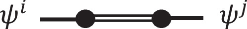
Figure 1. Diagram of generating kinetic mixing of SM fermion ψi . The double line represents the bulk and mirror fermion propagator.
Download figure:
Standard image High-resolution imageWe can evaluate these terms (14) by computing the bulk and mirror fermion propagator  and the summation of the KK modes. The methods are summarized in appendices A and B. The results are classified into three cases depending on the cases where a and b are the bulk fermion or the mirror fermion, and can be rewritten by the following functions,
where x = π
RpE
and  describes the distance between r1
i
and r2
j
. δ takes 0 if
describes the distance between r1
i
and r2
j
. δ takes 0 if  ) and 1 if
  . T denotes the periodicity of the fields. T = 1 corresponds to
  and T = − 1 corresponds to
  in tables 2, 3 and 4.
Table 1. Representation of bulk fermions and the corresponding mirror fermions. Pi is the parity of bulk fermion for i representation in SU(6). R in R(+,+) means an SU(6) representation of the bulk fermion. ri in r1 ⊕ r2 are SU(5) representations.
| Bulk fermion SU(6) → SU(5) | Mirror fermion |
|---|---|
| 20(+,+)=10 ⊕ 10* | 20(−,−) |
| 15(+,+)=10 ⊕ 5 | 15(−,−) |
|

|
| 6(−,−)=5 ⊕ 1 | 6(+,+) |

|

|
Table 2.
20 bulk and SM fermions. r1,2 in  are SU(3) and SU(2) representations in the SM, respectively. a is
  charges.
Bulk fermion 
| SM fermion coupling to bulk |
|---|---|

|

|

|

|
Table 3. Upper (Lower) table shows 15 ( ) bulk and SM fermions. r1,2 in
  are SU(3) and SU(2) representations in the SM, respectively. a is
  charges.
Bulk fermion 
| SM fermion coupling to bulk |
|---|---|

|

|

|

|
Bulk fermion 
| SM fermion coupling to bulk |

|

|

|

|
Table 4. Upper (Lower) table shows 6 ( ) bulk and SM fermions. r1,2 in
  are SU(3) and SU(2) representations in the SM, respectively. a is
  charges.
Bulk fermion 
| SM fermion coupling to bulk |
|---|---|

|

|

|

|
Bulk fermion 
| SM fermion coupling to bulk |
|
|
|

|
The first case is that both are bulk fermions:
where λ = π RM.
The second case is that they are bulk and mirror fermions, respectively:
The third case is that both are mirror fermions:
If some bulk and mirror fermions are introduced, all of the contributions to the kinetic and mass mixing must be summed in equation (14),


In the expression above, the superscript 'a' in  and Ma,ij
denotes the SU(6) representations and
and Ma,ij
denotes the SU(6) representations and  and Ma,ij
show the contributions from the corresponding bulk and mirror fermions.
and Ma,ij
show the contributions from the corresponding bulk and mirror fermions.
These kinetic mixing can be diagonalized by unitary matrices 


where  are diagonal matrices. After rewriting the mass term in terms of the new basis diagonalizing the kinetic mixings and normalizing the kinetic term, we obtain the following mass matrix

Next, we perform unitary transformations in order to move on to the mass basis:

In this new basis, the mass matrix is diagonalized:

This expression allows us to compute the SM fermion masses.
3.2. Weak interaction for the boundary fermion
As in the previous section, taking into account the mixing effects between the bulk and mirror fermions and the boundary fermions, additional mixing in the charged weak interaction of the boundary fermion, which is not present in the SM, also seems to be generated. The corresponding interactions generating the additional mixings in the charged weak interaction are shown below,
where W is the weak boson, u is up-type quark or electron and d is a down-type quark or neutrino. χ and  are the bulk and mirror fermions, respectively. Note that an
was defined as the corresponding 4D fields of the bulk or mirror fermions and we have not specified whether an
represents bulk or mirror fermions here. We will consider three cases as in the previous subsection and specify what an
is.
are the bulk and mirror fermions, respectively. Note that an
was defined as the corresponding 4D fields of the bulk or mirror fermions and we have not specified whether an
represents bulk or mirror fermions here. We will consider three cases as in the previous subsection and specify what an
is.
The additional generation mixing in the charged weak interaction is generated by integrating out the bulk and mirror fermions and can be seen from the diagram shown in figure 2,

where

Similarly, this contribution can be evaluated by using the method in appendices A and B. Here, we consider three cases where we specify whether an
is the bulk fermion χn
or the mirror fermion  . As a result, we find the additional mixings in the charged weak interaction to be the same as the kinetic mixing for the left-handed fermions localized on the boundary,

This property ensures that no additional mixing is needed, as will be shown below. In the case where some bulk and mirror fermions are introduced, the kinetic and mass mixing are the summation of all contributions in equation (29),

After rewriting the charged weak interaction in terms of the new basis in equation (25), the Cabibbo–Kobayashi–Maskawa (CKM) and Pontecorvo–Maki–Nakagawa–Sakat (PMNS) matrices are given by
where u, d, e and ν denote the up-type quarks, down-type quarks, charged leptons and neutrinos of the SM fermion, respectively. We utilized the fact that the contributions of the left-handed SU(2) doublets to the kinetic mixing are the same, for instance,  and
and  . These expressions allow us to calculate the weak mixing angles and a CP phase.

Figure 2. Diagram of the generation of the weak interaction of an SM fermion. ψi and W are the SM fermion and the weak boson, respectively. The double line represents the bulk and mirror fermion propagator.
Download figure:
Standard image High-resolution image
3.3. Fermion sector of our model and results
In the setup of our model, we introduce five bulk fermions  and the corresponding mirror fermions
  shown in table 1. Note that the number of bulk fermions has been reduced from nine in [10] to five, which necessarily introduces generational mixings through the coupling of bulk fermions to boundary fermions. The Lagrangian for the bulk and mirror fermions is given by

where the subscript a denotes the SU(6) representations of the bulk and mirror fermions. The bulk masses between the bulk and the mirror fermions are normalized by π R and expressed by the dimensionless parameter λa .
The SM quarks and leptons for the first and the second generation are embedded into SU(5) multiplets localized at the y = 0 boundary, which are two sets of decouplets, anti-quintets and singlets  . On the other hand, those for the third generation are embedded into
  multiplets localized at the y = π
R boundary. The reason why such a configuration of the SM fermions is adopted is to avoid massless SM quarks and leptons. If three generations of the SM fermions are localized on the y = 0 boundary, we found that the rank of the mass matrices for the SM quarks and leptons is at most two, which means that at least one massless quark or lepton is inevitable. Therefore, the Lagrangian for the SM fermions
multiplets localized at the y = π
R boundary. The reason why such a configuration of the SM fermions is adopted is to avoid massless SM quarks and leptons. If three generations of the SM fermions are localized on the y = 0 boundary, we found that the rank of the mass matrices for the SM quarks and leptons is at most two, which means that at least one massless quark or lepton is inevitable. Therefore, the Lagrangian for the SM fermions  is expressed by
Here, the superscript 'j' denotes the generation of the SM fermions and  is the Dirac conjugate of χb
.
is the Dirac conjugate of χb
.
In order to realize the SM fermion masses, the boundary localized mass terms between the SM fermions localized at the boundaries and the bulk fermions are necessary. To allow such localized mass terms, we have to choose appropriate SU(6) representations for bulk fermions carefully. Note that, for simplicity, the mirror fermions have no coupling to the SM fermions in this setup.  are boundary mass terms between the bulk fermions and the SM fermions, which are defined as follows.
where ΨM⊂N
is a bulk fermion for M in SU(5) representation and N means SU(6) representation.  is the strength of the mixing term between the bulk fermion and the SM fermion and should be a complex number to avoid the problem where the determinant of the mass matrix in equation (18) equals zero. In other words, some SM fermions become a massless state. The decomposition of the introduced bulk fermions in the 20, 15 (
 ), 6 (
 ) representations into the SM gauge group and the corresponding the SM fermions to be coupled on the boundary are summarized in tables 2, 3 and 4, respectively.
Based on the discussion above, our total Lagrangian for the fermions is given as follows:

Solving the exact KK spectrum of the bulk fermions from this Lagrangian is very difficult because of the complicated bulk and boundary system. We assume in this paper that the physical mass induced for the boundary fields is much smaller than the masses of the bulk fields [7]. This is reasonable since the compactification scale and the bulk mass mainly determines the KK mass spectrum of the bulk fields is larger than the mass for the boundary fields whose typical scale is given by the Higgs VEV. In this case, the effects of the mixing on the spectrum for the bulk fields can be negligible and the spectrum  is a good approximation [7].
Thanks to the reduction of bulk fermions, we can reproduce the quark and lepton mixing angles in addition to the SM fermion masses. For example, the discussion in section 3.1 allows us to obtain up-type quark mass Mu in the following form
where c = c1 + c2, and  are the input parameters that appeared in equations (35) and (36). Λij
(i, j = 1, 2, 3) is defined as
are the input parameters that appeared in equations (35) and (36). Λij
(i, j = 1, 2, 3) is defined as  ,
,  and
and  . Mass matrices for other types of quarks and leptons are given in a similar way. After following the method discussed in section 3.2, we can also calculate the flavor-mixing angles and a CP phase and fit them to their experimental values. This is because we have now changed the way the bulk fermions couple to the SM fermions. In the previous model, each type of bulk fermion was introduced per generation so that the mass matrices were essentially diagonal.
Finally, we have identified allowed parameter sets capable of reproducing the SM fermion masses and mixing. Sample data sets depending on the parameter of the localized gauge kinetic terms c are shown in tables 5, 6 and 7. Note that we use experimental data in our analysis and one of the standard conventions for the CKM and PMNS matrices shown by the Particle Data Group [13]. In the analysis of the neutrino sector, we assume a normal hierarchy, although it is not a mandatory requirement. As can be seen from tables 5 and 6, our results are in almost good agreement with the experimental data. 7 This is a very remarkable result since it introduces new generation mixing in the bulk resulting from the reduction of the number of bulk fermions, which makes, in particular, reproducing the quark and lepton mixing angles highly nontrivial. Our model turned out to be a good starting point for constructing a realistic model of GGHU.
Table 5. Our results of parameter fitting in the quark sector for some parameters 1/R and c = c1 + c2. The up, down and strange quark masses are the  masses at the scale μ=2 GeV. The charm and bottom quark masses are the
  masses renormalized at the
  mass, i.e.
  . The top quark mass is extracted from direct measurements.
| 1/R | c | mu | mc | mt | |
|---|---|---|---|---|---|
| 10 TeV | 80 | 2.163 MeV | 1.217 GeV | 166.294 GeV | |
| 10 TeV | 90 | 2.320 MeV | 1.229 GeV | 167.931 GeV | |
| 15 TeV | 80 | 2.316 MeV | 1.214 GeV | 165.300 GeV | |
| 15 TeV | 90 | 2.156 MeV | 1.225 GeV | 166.89 GeV | |
| Data |
 MeV MeV | 1.27 ± 0.02 GeV | 172 ± 0.30 GeV |
| 1/R | c | md | ms | mb | |
|---|---|---|---|---|---|
| 10 TeV | 80 | 5.583 MeV | 75.7 MeV | 4.155 GeV | |
| 10 TeV | 90 | 5.505 MeV | 75.8 MeV | 4.321 GeV | |
| 15 TeV | 80 | 5.522 MeV | 75.5 MeV | 4.201 GeV | |
| 15 TeV | 90 | 5.545 MeV | 75.1 MeV | 4.183 GeV | |
| Data |
 MeV MeV |
 MeV MeV |
 GeV GeV |
| 1/R | c |

|

|

| δ |
|---|---|---|---|---|---|
| 10 TeV | 80 | 0.191 797 | 0.003 537 | 0.041 430 | 1.1560 |
| 10 TeV | 90 | 0.195 857 | 0.003 510 | 0.039 893 | 1.2424 |
| 15 TeV | 80 | 0.190 839 | 0.003 556 | 0.041 459 | 1.1831 |
| 15 TeV | 90 | 0.192 085 | 0.003 518 | 0.040 088 | 1.1750 |
| Data | 0.226 50 ± 0.00048 |

|

|

|
Table 6. Our results of parameter fitting in the lepton sector for some parameters 1/R and c = c1 + c2. In the neutrino sector, a normal hierarchy is assumed.
| 1/R | c | me | mμ | mτ |
|---|---|---|---|---|
| 10 TeV | 80 | 0.5136 MeV | 98.750 MeV | 1687.12 MeV |
| 10 TeV | 90 | 0.5140 MeV | 98.188 MeV | 1689.56 MeV |
| 15 TeV | 80 | 0.5135 MeV | 98.776 MeV | 1695.46 MeV |
| 15 TeV | 90 | 0.5139 MeV | 98.610 MeV | 1687.59 MeV |
| Data | 0.510 998 946 1(31) MeV | 105.658 374 5(24) MeV | 1776.86(12) MeV | |
|---|---|---|---|---|
| 1/R | c |

|
 (Normal) (Normal) | δ |
| 10 TeV | 80 | 7.7306 × 10⁻⁵ eV2 | 2.4524 × 10⁻³ eV2 | 1.539π rad |
| 10 TeV | 90 | 7.7087 × 10⁻⁵ eV2 | 2.4367 × 10⁻³ eV2 | 1.536π rad |
| 15 TeV | 80 | 7.8054 × 10⁻⁵ eV2 | 2.3895 × 10⁻³ eV2 | 1.531π rad |
| 15 TeV | 90 | 7.6544 × 10⁻⁵ eV2 | 2.4577 × 10⁻³ eV2 | 1.536π rad |
| Data | (7.53 ± 0.18) × 10−5 eV2 | (2.453 ± 0.033) × 10−3 eV2 |
 rad rad | |
|---|---|---|---|---|
| 1/R | c |

|

|
 (Normal) (Normal) |
| 10 TeV | 80 | 0.3313 | 2.240 × 10⁻² | 0.5161 |
| 10 TeV | 90 | 0.3294 | 2.155 × 10⁻² | 0.5187 |
| 15 TeV | 80 | 0.3505 | 2.094 × 10⁻² | 0.5069 |
| 15 TeV | 90 | 0.3308 | 2.123 × 10⁻² | 0.5161 |
| Data | 0.307 ± 0.013 | (2.20 ± 0.07) × 10−2 | 0.546 ± 0.021 | |
Table 7. Input parameters of the parameter fitting where c = c1 + c2.  are the bulk masses between the bulk and the mirror fermions which are normalized by π
R. is the strength of the mixing term between the bulk fermion and the SM fermion, ∣∣ is its absolute value and θ is a phase of the corresponding . Only
are the bulk masses between the bulk and the mirror fermions which are normalized by π
R. is the strength of the mixing term between the bulk fermion and the SM fermion, ∣∣ is its absolute value and θ is a phase of the corresponding . Only  can be taken as a real number without loss of generality. This is because we have not shown
  in this table.
| 1/R | c | λ20 | λ15 |

| λ6 |

|
|---|---|---|---|---|---|---|
| 10 TeV | 80 | 0.697 103 | 0.379 299 | 1.866 68 | 13.404 | 12.0452 |
| 10 TeV | 90 | 0.707 565 | 0.382 020 | 1.875 16 | 13.383 | 12.0376 |
| 15 TeV | 80 | 0.727 571 | 0.421 544 | 1.885 62 | 13.390 | 11.0374 |
| 15 TeV | 90 | 0.737 359 | 0.428 899 | 1.896 30 | 13.355 | 11.0374 |
| 1/R | c |

|

|

|

|

|
|---|---|---|---|---|---|---|
| 10 TeV | 80 | 1 | 0.061 893 8 | 0.398 107 | 0.000 724 436 | 0.020 417 4 |
| 10 TeV | 90 | 1.000 05 | 0.062 408 1 | 0.398 146 | 0.000 668 344 | 0.019 724 2 |
| 15 TeV | 80 | 0.999 60 | 0.062 089 9 | 0.398 107 | 0.000 031 622 8 | 0.006 683 44 |
| 15 TeV | 90 | 0.999 994 | 0.062 593 | 0.398 095 | 0.000 029 512 1 | 0.006 531 31 |
| 1/R | c |

|

|

|

|

|
|---|---|---|---|---|---|---|
| 10 TeV | 80 | 0.190 546 | 0.014 150 8 | 0.079 432 8 | 0.000 426 58 | 0.010 115 8 |
| 10 TeV | 90 | 0.190 545 | 0.014 177 3 | 0.079 433 3 | 0.000 380 189 | 0.009 885 53 |
| 15 TeV | 80 | 0.190 546 | 0.014 159 3 | 0.079 432 8 | 0.000 028 510 2 | 0.004 954 5 |
| 15 TeV | 90 | 0.190 546 | 0.014 197 0 | 0.079 433 1 | 0.000 026 607 3 | 0.004 841 72 |
| 1/R | c |

|

|

|

|

|
|---|---|---|---|---|---|---|
| 10 TeV | 80 | 0.007 368 13 | 0.258 731 | 0.070 371 2 | 5.956 450 | 3.783 11 |
| 10 TeV | 90 | 0.007 449 81 | 0.253 490 | 0.071 090 4 | 5.956 450 | 3.783 11 |
| 15 TeV | 80 | 0.007 758 07 | 0.268 290 | 0.073 149 7 | 0.712 979 | 4.940 97 |
| 15 TeV | 90 | 0.007 744 13 | 0.263 562 | 0.074 399 5 | 0.752 089 | 4.940 97 |
| 1/R | c | ∣20e
∣ | ∣15u
∣ |

| ∣6ν
∣ |

|
|---|---|---|---|---|---|---|
| 10 TeV | 80 | 0.054 238 6 | 0.000 873 495 | 0.008 777 01 | 0.000 01 | 0.000 01 |
| 10 TeV | 90 | 0.052 238 6 | 0.000 847 602 | 0.008 491 88 | 0.000 010 115 8 | 0.000 01 |
| 15 TeV | 80 | 0.054 210 9 | 0.000 878 758 | 0.008 885 08 | 0.000 213 796 | 0.000 01 |
| 15 TeV | 90 | 0.051 966 0 | 0.000 853 353 | 0.008 584 60 | 0.000 211 349 | 0.000 01 |
| 1/R | c | θ20e | θ15u |

| θ6ν |

|
|---|---|---|---|---|---|---|
| 10 TeV | 80 | 4.251 55 | 4.147 07 | 4.213 75 | 3.180 33 | 0.000 01 |
| 10 TeV | 90 | 4.226 78 | 4.165 61 | 4.214 89 | 3.180 33 | 0.000 01 |
| 15 TeV | 80 | 4.289 15 | 4.111 34 | 4.223 85 | 4.560 62 | 0.000 01 |
| 15 TeV | 90 | 4.286 32 | 4.129 57 | 4.2136 | 4.560 62 | 0.000 01 |
| 1/R | c | ∣20q
∣ | ∣15e
∣ | θ20q | θ15e | |
|---|---|---|---|---|---|---|
| 10 TeV | 80 | 0.011 359 9 | 0.001 225 72 | 2.155 76 | 2.163 23 | |
| 10 TeV | 90 | 0.010 911 6 | 0.001 965 32 | 2.137 19 | 2.595 40 | |
| 15 TeV | 80 | 0.011 597 6 | 0.001 235 53 | 2.193 91 | 2.572 35 | |
| 15 TeV | 90 | 0.011 416 7 | 0.001 407 87 | 2.175 91 | 2.651 10 |
Note that these parameters are evaluated at the compactification scale. In order to compare these values with the experimental data, we have to solve the renormalization group equation (RGE) from the compactification scale ( TeV) to the weak scale, but we expect that these RGE effects do not affect our results.
4. Conclusions
In this paper, we have discussed the fermion mass hierarchy and mixing in SU(6) GGHU with localized gauge kinetic terms. The SM fermions are introduced on the boundaries. We also introduced massive bulk fermions in three types of SU(6) representations coupling to the SM fermions on the boundaries. Their number has been reduced in order to achieve generation mixings of quarks and leptons, which greatly changed the coupling of the bulk fermions to the SM fermions on the boundaries and led to the appearance of additional generation mixings in the bulk sector. This feature makes our analysis of the SM fermion masses and mixing angles highly complicated and nontrivial. We have shown that the SM fermion masses and mixing can be almost reproduced by mild tuning of bulk masses and the parameters of the localized gauge kinetic terms. Some parameter sets of our results are listed. The model discussed in this paper turned out to be a good starting point for constructing a realistic model of GGHU.
For our future work, it is important to calculate the effective potential for the Higgs field and study whether the electroweak symmetry breaking occurs correctly. Since the Higgs field is originally a gauge field, the potential is generated at the one-loop level by the Coleman–Weinberg mechanism. It is not easy to obtain the observed Higgs mass 125 GeV because the effects of localized gauge kinetic terms enhance the compactification scale and Higgs boson mass. From the viewpoint of gauge coupling unification, we have little room to introduce extra bulk fields to adjust the Higgs mass, which also makes the analysis of the electroweak symmetry breaking difficult. It is possible to introduce a Majorana neutrino on the boundary in order to obtain the Higgs boson mass, which relaxes the constraint for the bulk mass parameters. We would like to investigate the electroweak symmetry breaking and Higgs boson mass along this line. The predictions from this model could be also studied based on these analyses.
Acknowledgments
This work was supported by JST SPRING, Grant Number JPMJSP2139 (Y Y ).
Data availability statement
All data that support the findings of this study are included within the article (and any supplementary files).
Appendix A.: The propagator of the bulk and mirror fermion
The bulk and mirror fermions  in five dimensions and their KK decomposition is given by
where  are 4D fields and fn
(y) is a mode function. The quadratic terms for
are 4D fields and fn
(y) is a mode function. The quadratic terms for  can be expressed in momentum space by using the above KK decomposition as

which leads to the propagator in Minkowski spacetime

or in Euclidean spacetime

Appendix B.: Summation of the KK mode
In order to evaluate equation (14), we need to calculate the summation of KK mode contributions. The summation of KK mode contributions can be rewritten as
where δ = 0(1) for the case where the left-handed and right-handed boundary fermions are localized on the same (opposite) boundary. T is the periodicity for bulk and mirror fermions. The factor n + ν + q α in the denominator comes from the KK mass spectrum

where α is a dimensionless parameter corresponding to the VEV of the Higgs field.
Furthermore, it is useful to express the real and imaginary part of these functions.
therefore we obtain
Footnotes
- 5
For earlier attempts and related works, see [5].
- 6
In the case of SU(6) GGHU in warped space [6], a realistic spectrum is realized fully due to appropriate boundary terms with suitable bulk representations.
- 7
We managed to find the input parameters to reproduce the output parameters with the present accuracy. It is difficult to find all regions of allowed parameters. That is why ms and the Cabibbo angle look to be considerably different. It is expected that there exist sets of input parameters that will enable us to obtain the output parameters more accurately. We could find such input parameters after improving analysis methods.