
Abstract
A high temperature superconducting (HTS) demonstration coil has been developed in the frame of the Experimental Physics department Research and Development program at CERN The magnet extends the recent experimental demonstration of aluminium-stabilised HTS conductors and supports the development of future large scale detector magnets. The HTS magnet has five turns and an open bore diameter of 230 mm. Up to 30 K, the coil was measured to be fully superconducting across four central turns at 4.4 kA, the maximum available current of existing power supply. The central magnetic field is 0.113 T, the peak field on the conductor is 1.2 T and the coil has a stored magnetic energy of 0.1 kJ. A 3D-printed aluminium alloy (Al10SiMg) cylinder acts both as a stabiliser and a mechanical support for the superconductor. The resistivity of Al10SiMg was measured at cryogenic temperatures, and has a residual resistivity ratio of approximately 2.5. The ability to solder ReBCO tapes (a stack of four REBCO tapes, 4 mm wide, Fujikura) to Al10SiMg stabiliser, electroplated with copper and tin, forming a coil, is demonstrated using tin-lead solder at 188 ∘C. The HTS magnet was proven to be stable when superconductivity was broken locally using a thin-film heater. Despite voids in the solder joint between HTS and stabiliser, no degradation of the magnet's performance was observed after 12 thermal cycles and locally quenching the magnet. A numerical model of the transient behaviour of solenoid with partially shorted turns is developed and validated against measurements. Our work experimentally and numerically validates that using an aluminium alloy as a stabiliser for HTS tapes can result in a stable, lightweight and transparent magnet.
Export citation and abstract BibTeX RIS

Original content from this work may be used under the terms of the Creative Commons Attribution 4.0 license. Any further distribution of this work must maintain attribution to the author(s) and the title of the work, journal citation and DOI.
1. Introduction
This magnet, developed as part of CERN EP R&D for future detector magnets, serves as a demonstrator for projects needing ultra-thin, radiation transparent, light-weight and self-protected magnets, to be operated without liquid helium. It uses ReBCO high-temperature superconductor (HTS) soldered to a 3D-printed aluminium cylinder which acts as a stabiliser for current-sharing in case of a quench and support for the Lorentz-forces. Aluminium is chosen due to its low density and thus high radiation transparency, which is a requirement for detector magnets where the magnet is between the interaction point and the calorimeter. ReBCO as a conductor allows for operation at elevated temperatures, which is not only advantageous because of the present and expected future helium shortage [1, 2], but also for projects such as AMS-100 [3] where operation at elevated temperatures is a necessity. Furthermore, following Carnot efficiency, operation at higher temperatures saves cooling costs compared to low temperature superconductors (LTSs).
Conventionally, pure aluminium or pure copper is used for stabilisation of LTS Nb–Ti cables due to its low electrical resistance and high thermal conductivity at cryogenic temperatures. At elevated temperatures, where HTS-magnets can be operated, these pure metals however loses some of these advantages with respect to alloys [4].
This HTS magnet extends the recent experimental demonstration of aluminium-stabilised HTS cables [5, 6] and experimentally validates that an aluminium alloy with an impurity fraction as high as 10% can be used as a stabiliser for this type of partially-insulated HTS magnets. The mild transition edge and large temperature margin intrinsic to ReBCO compared to LTS allow for the usage of an aluminium alloy for stabilisation. Advantages of this stability are decreased risks of magnet training and degradation.
Using aluminium alloys as stabiliser for HTS has some advantages over pure aluminium, such as higher strength, lower costs, and better availability. With 3D-printing, complex shapes and fast-prototyping of aluminium structures are achievable. At this moment, However, in case of a quench, the higher resistivity of the stabiliser alloy leads to more heating and higher voltages [7], which are unfavourable. Despite that, this 3D-printed magnet, which has more than a factor 400 higher stabiliser resistivity at 4.2 K compared to the stabiliser used in the largest detector magnets ATLAS and CMS [8], proved to be stable, even when locally quenching. This was achieved by combining the aluminium stabiliser with partial insulation. Partial insulation is a passive quench protection technique where the stored energy is distributed by creating bypasses in between turns. Current can flow around the quenched region, decreasing the local hotspot temperature which makes this magnet 'self-protected': the cold mass can absorb the stored magnetic energy and keeps the hotspot temperature and the corresponding thermal stresses sufficiently low not to damage the magnet. It should be notes that the energy-density of this magnet operated at 4.5 kA is a factor 40 lower than ATLAS and CMS.
Along with detector magnets, this technology may be useful for applications where thin, exotically shaped, stable, light-weight and efficiently cooled HTS magnets are needed. For example, magnets for radiation-shielding or propulsion in space.
This paper continues in section 2 by presenting the design of the magnet and measurements of the electrical resistivity of Al10SiMg at cryogenic temperatures. In section 3, the manufacturing process of the HTS magnet is explained and section 4 describes the performance of the magnet at various temperatures and when locally breaking superconductivity. Section 5 presents results of a thermo-electromagnetic simulation of the transient behaviour of the magnet. Subsequently, measurements and simulations are compared in section 6 and conclusions are discussed in section 8.
2. Design of the magnet
The support cylinder design of our 230 mm diameter open-bore HTS magnet consists of 5 helical turns of a U-shape profile, connected to the neighbouring turns by 19 shorts per turn as partial insulation as shown in figure 1. These shorts are intentionally incorporated as part of the 3D-printed structure. A stack of four Fujikura FESC-SCH04 wires, each pre-coated with tin-lead, is soldered together to the U-groove. Properties corresponding to this design of the coil when operated at 4.5 kA are listed in table 1. A simulated axi-symmetric magnetic field map of a coil in this geometry at 4.5 kA is displayed in figure 2. Based on the simulation the peak magnetic field experienced by the ReBCO tapes is 1.2 T, the shear stress at 4.5 kA between the tapes and cylinder is maximum 0.45 MPa, which is significantly lower than the shear delamination strength of ReBCO ( 3 MPa) [9] and the yield strength of tin-lead solder (
 40 MPa) [10]. The chosen manufacturing method of the cylinder is 3D-printing because of its short lead time and capability to manufacture the desired shape. The material choice was governed by the manufacturing process. Despite that AlF357 and Al2139 alloys are possible to 3D-print, Al10SiMg was chosen because of its better availability and lower cost. The choice 3D-printing currently gives an upper limit to the size of the coil. However, the geometry shown in figure 1 is considered representative of a wound conductor where locally welds are made between adjacent conductors to allow axial current redistribution. Because the electrical resistivity of 3D-printed Al10SiMg was unknown at cryogenic temperatures, samples were measured for electrical resistivity from 4.2 K to room temperature, presented in the next section.

Figure 1. Frontal—top view of the coated cylinder before soldering (a) and inside view of the coil after soldering the tapes (b).
Download figure:
Standard image High-resolution image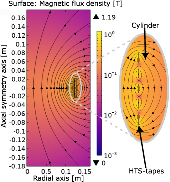
Figure 2. Simulated magnetic field map of a cylinder with azimuthal current in 5 turns at 4.5 kA. The colourmap represents the magnetic field in Tesla, and the arrowed contours illustrate magnetic field lines.
Download figure:
Standard image High-resolution imageTable 1. Properties of the HTS magnet.
| Design parameter | Value | Unit |
|---|---|---|
| Conductor | ||
| Conductor | 4 ReBCO tapes soldered in Al U-profile | |
| Aluminium | 3D-printed Al10SiMg | |
| HTS type | Fujikura FESC-SCH04 | |
 per tape at 77 K in self-field per tape at 77 K in self-field | 155 | A |
| Solder | Sn–Pb | |
| Coil | ||
| Inner diameter | 230 | mm |
| Length | 50 | mm |
| Number of shorts per turn | 19 | (—) |
| Width of short | 3.1 | mm |
| Thickness of cylinder wall | 5 | mm |
| Depth groove in U-profile | 2 | mm |
| Weight | 0.5 | kg |
| Inductance | 0.01 | mH |

| 5 | (—) |
| Central field | 0.114 | T |
| Peak field on conductor | 1.2 | T |
| Stored magnetic energy | 0.1 | kJ |
| Energy density | 0.2 | kJ kg−1 |
2.1. Cryogenic properties of Al10SiMg
As the stabiliser carries the current in case of a quench and resistive heating influences the superconducting characteristics, it is useful to know the electrical and thermal resistivity of the used material at a range of temperatures. To determine the electrical resistivity of Al10SiMg, test samples with a cross-section of 20 mm  10 mm from two different manufacturers were printed (Xometry and IN3DTEC). The current-to-voltage characteristics of these samples were measured across a distance of 100 mm at temperatures from 4.2 K to room-temperature to obtain the corresponding electrical resistivities with temperature shown in figure 3. In addition to these measurement results, Bloch–Gruneisen fits of resistivity data of pure aluminium [11] and 99% pure aluminium alloy (Al 1100) [4] are depicted for comparison. From this was extracted that Al10SiMg has a residual resistivity ratio of around 2.5.

Figure 3. Measured resistivity from 4.2 K to room temperature of two 3D-printed Al10SiMg samples compared to pure aluminium data from [11] and aluminium alloy (Al 1100) data from [4].
Download figure:
Standard image High-resolution imageThe additive manufacturing process of Al10SiMg results in an anisotropic microstructure of the alloy. Near grain boundaries of as-built samples, regions having high concentration of silicon were identified and the direction of grain growth was observed to depend on the build orientation causing anisotropic electrical resistivity [12]. Since the microstructure is not exactly known, the impurity fraction is significantly higher than 5%, and the temperature dependence of the resistivity of the predominant metal and the alloying elements are different, no simple estimations of the direction dependence of the resistivity at cryogenic temperatures could be made. Therefore, we measured the resistivity of Al10SiMg perpendicular and parallel to the build orientation at room temperature and 77 K shown in figure 4.
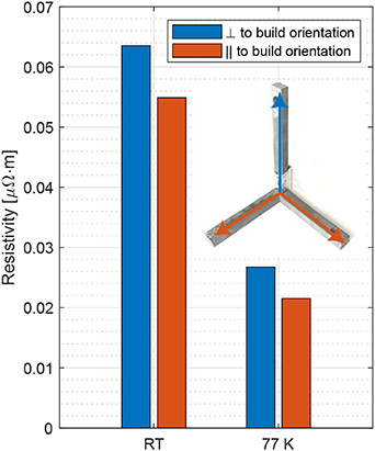
Figure 4. Measured build orientation dependence of Al10SiMg electrical resistivity at 77 K and room temperature alongside a picture of the test piece printed by Xometry with arrows indicating the direction of resistivity.
Download figure:
Standard image High-resolution imageIn accordance with earlier studies, resistivity is higher in the direction perpendicular to build orientation compared to parallel, indicated by the blue and orange arrows respectively in figure 4. At room temperature, the piece has a 14% higher resistivity in the perpendicular direction compared to parallel, and this increases at 77 K to 19%. It should be noted that this effect was measured on the same piece, thereby excluding material variability. Because of the difference between resistivity values for the two different manufacturers as shown in figure 3, this material uncertainty must be considered separately.
We estimate the thermal conductivity from the electrical resistivity ρ by the Wiedemann–Franz approximation because a direct measurement of thermal conductivity would require a dedicated instrumentation.
where k depicts the thermal conductivity, T is the temperature and L is the Lorentz ratio. For aluminium alloys, except the relatively pure 1100 and 2024 series, it is shown that Lorentz ratios are constant within ±10% of the Sommerfeld value [4]. Therefore, we assume that for this diluted alloy, this is also the case and that the thermal conductivity can be estimated using equation (1) within 10%–20% accuracy.
3. Fabrication of the magnet
3.1. Coating of the support cylinder
To ensure current-sharing between the superconductor and stabiliser and for the mechanical support of the tapes, the superconducting ReBCO tapes are soldered to the cylinder. To solder directly to aluminium, temperatures over 280 ∘C would be needed to remove the refractory oxide on the surface with reactive chloride fluxes [10]. Exposure to this temperature would permanently degrade the performance of the tapes [13, 14]. Next to that, aluminium specific solders flow poorly, and aluminium reacts with Sn–Pb solders causing corrosion at the solder interface [10] leading to bad contact. To avoid degradation by temperature and mentioned concerns, it was decided to first coat the cylinder electrochemically and later solder the tapes to this coating. The first layer of the coating enables bonding between copper and aluminium and consists of  –
– m nickel. The second layer consists of 10–
 m copper for current-sharing and the last layer consists of
  m tin to prevent the copper from oxidising. This way, the tapes can be soldered to the support cylinder at a temperature of 188 ∘C without degradation.
3.2. Soldering of the ReBCO tapes
For soldering the tapes to the coated cylinder, we used a similar method as for cables described by [5], but the type of solder is changed from tin-bismuth (Sn 42%, Bi 57.6%, Ag 0.4%) to tin-lead (Sn 63%, Pb 37%). The higher melting temperature of Sn–Pb allows us to use Sn–Bi to make a low-resistance solder joint between the current-leads and the cylinder without melting the tape-to-cylinder solder joint.
Both ends of the stack of tapes are trimmed in a staircase pattern with each Hastelloy layer pointed away from the aluminium. This way, each tape end has 4 mm × 20 mm direct contact with the coated aluminium lowering the contact resistance to each ReBCO layer. Measurements comparing a stack of four ReBCO tapes from the same spool soldered to the same electrochemically coated stabiliser with these two different solders (Sn–Bi at 160 ∘C and Sn–Pb at 188 ∘C) did not show an observable degradation in  . The degradation, if any, was smaller than the
  fluctuation within the same tape at 77 K.
To fix the tapes in the helical U-profile of the cylinder during soldering, a Teflon tube is pressed against the ReBCO tapes from the inside of the cylinder using stainless-steel parts. Everything was soldered in an air drying oven which was heated to 188 ∘C for 6 h and then switched off to obtain a gradual cool-down. After soldering, the tube and stainless-steel parts were removed. Figure 1(b) shows the tapes already soldered to the groove of the cylinder.
To non-destructively investigate the soldering quality, a computed tomography scan of the coil was taken. The scan indicates the presence of voids in the solder joint between the cylinder and tapes, some highlighted by red ellipses in figure 5 [15]. The formation of voids may be prevented by soldering in a vacuum oven. Despite the presence of voids, the HTS magnet performed to expectations, as described in the next sections.
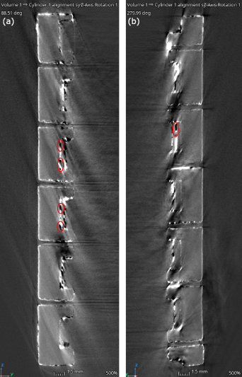
Figure 5. CT-scans of two cross-sections of the cylinder after soldering the HTS-tapes. Solder (high-density) is displayed as white, and voids can be identified as black spots, some highlighted by red ellipses.
Download figure:
Standard image High-resolution image3.3. Current lead assembly
Current leads of our HTS coil consist of two oxygen-free electronic (OFE) copper rings with a groove. The ends of the cylinder are soldered in the grooves of the rings with Sn–Bi. After soldering, additional stainless-steel rods were inserted in the current leads to insure mechanical protection of the soldered joints as can be seen in figure 6. These current leads are subsequently clamped to the busbars of our existing liquid helium cryostat using OFE-copper adaptor pieces and indium tape.

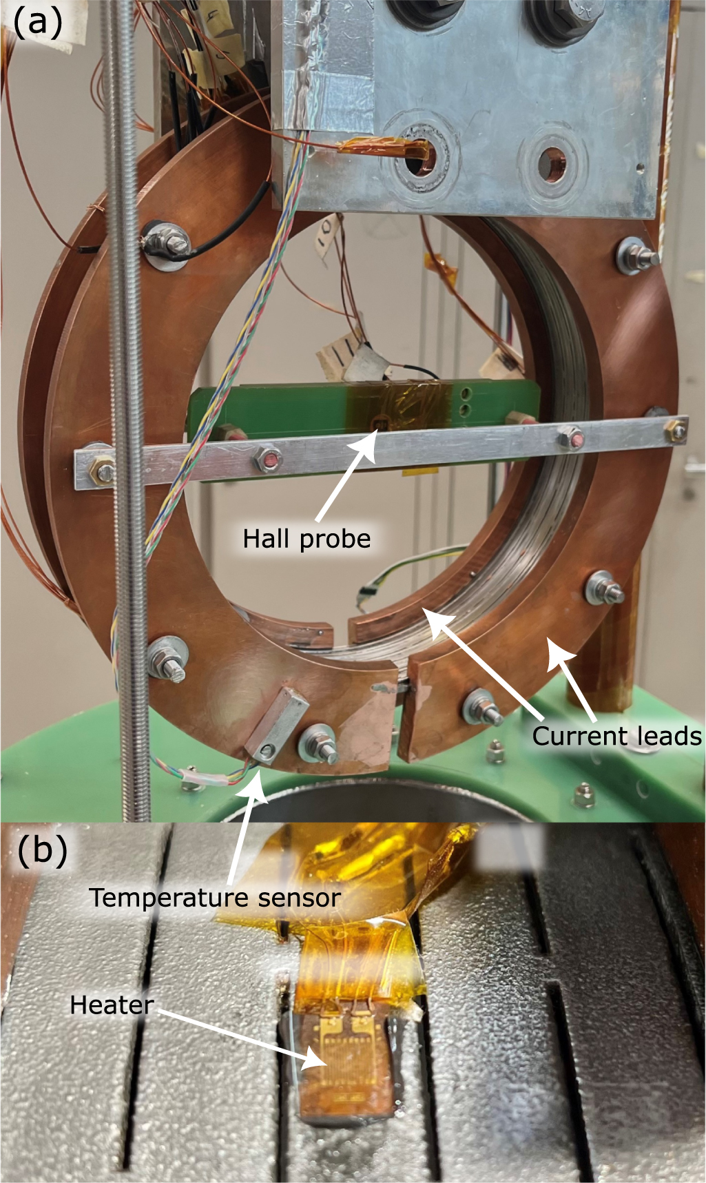
Figure 6. Al-stabilised HTS magnet mounted to the busbars of the helium cryostat (a) and the quench initiate heater glued to the cylinder (b).
Download figure:
Standard image High-resolution image4. Measured performance of the magnet
4.1. Setup and instrumentation
The magnet's performance was measured in liquid nitrogen, gaseous helium and liquid helium. For testing at 77 K, the magnet was submerged in a liquid nitrogen dewar and powered by two Delta Elektronika SM 15-400 power supplies connected in parallel providing a maximum current of 800 A.
The HTS magnet was also tested in a helium cryostat for operation in liquid or gaseous helium. In this setup the busbars were connected to a 4.5 kA Magna-Power Electronics MSA5-4500/380 power supply via He gas cooled current leads. Due to vertical orientation of the magnet in the cryostat, it will see the temperature gradients in the gaseous helium.
Across the four middle turns of the coil, voltage taps were positioned every half turn, resulting in eight half-turn sections across which the voltage can be independently measured. Additionally, voltage taps were attached to the current leads allowing for junction resistance measurements needed to estimate the contact heat load.
In the centre of the magnet, an AREPOC s.r.o. Hall probe is placed and two bridge temperature sensors [16] were mounted on a current lead. One was positioned at the top of the lead, the other at the bottom. Direct attachment to the coil would result in a poor contact given the mismatch in the round surface of the coil and the flat surface of the temperature sensor. The lead is assumed to give an indication of the temperature of the coil given the soldered connection. A thin-film heater with a cross-section of  was glued to the aluminium at the bottom of the coil using a thermally-conductive epoxy, shown in figure 6(b).
Voltages were measured with both a Keithley DAQ6510 scanning multimetre and 34401A multimetres in parallel and the operating current of the magnet is measured using a 20  room-temperature shunt-resistor in series.
4.2. Measurements in liquid nitrogen
Using the  V m−1 convention, a critical current at 77 K
  = (
= ( ) A was extracted from a power-law fit of the current–voltage characteristics depicted in figure 7. When looking at the magnetic field shown in the same figure, it can be observed that up to 550 A the field increases linearly with increasing current. Around 580 A however, the limit of the tapes is at least locally reached and the current redistributes as the field does not increase linearly with the current anymore. For this magnet, the voltage increases almost linearly after reaching the limit of the tapes, corresponding to the resistance of the stabiliser.
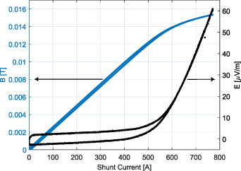
Figure 7. Electric field across the magnet and central magnetic field plotted against current at 77 K. The current was ramped up and down at a rate of 1 A s−1.
Download figure:
Standard image High-resolution imageAnalysis of the response of the magnetic and voltage to a step up and down in current, shown in figure 8 gives a time constant  s, where the expanded uncertainty is determined from the fitted values from various current levels between 200–800 A. It is noteworthy to mention that when current-redistribution has taken place after a step up from 0 at 600–800 A, the developed voltage does not runaway as shown in figure 8(b) allowing stable operation of the magnet.
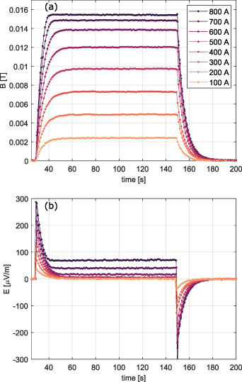
Figure 8. Response to a step up and down in current of B-field in the centre of the HTS coil (a) and electric field across 4 turns (b) for a range of currents.
Download figure:
Standard image High-resolution image4.3. Measurements in liquid and gaseous helium
Before measuring in helium, the magnet was thermally cycled for 10 times between 77 K and room temperature. Afterwards, it was measured twice at 4.2 K and no changes in the central magnetic field or voltage were observed. At a current of  A, the B-field in the centre of the HTS coil was measured to be
  T. The inductance L of 4 turns
  H. The inductance is determined from the difference in induced voltage
  when ramping up and down the magnet with rate
  as
as
The total inductance, including the copper current leads, is  = (9.0 ± 0.4) µH.
The critical current of the magnet was measured from 30 to 77 K, with the lower temperature limit imposed by the maximum current of 4.5 kA of the power supply used. Figure 9 depicts the measured critical current, defined at an electric field of  V m−1, as function of the effective temperature and a trendline based on scaling and offsetting the critical current of an individual tape at 3 T provided by Fujikura [17].
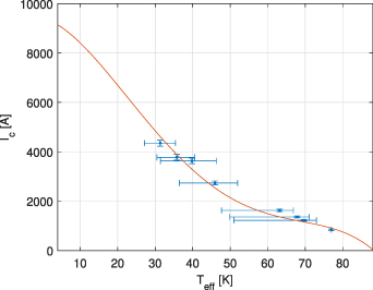
Figure 9. Measurements and trendline of the HTS magnet critical current as function of effective temperature. The displayed limits for the temperature are the measured temperature at the bottom and top of the current lead of the coil. We estimate the 2σ uncertainty in effective temperature to be lower, that is ±3.3 K.
Download figure:
Standard image High-resolution imageEffective temperature consists of a scaling of the measured temperature at the top and bottom of the current lead with the dependence of critical current of an individual tape. The critical current has a the strong temperature dependence and the large ±10 K vertical temperature gradients were measured across the HTS coil with the bridge sensors attached to the current lead. If we assume a linear temperature gradient, the temperature profile along the coil can be described as:
where  is the average temperature,
  is the temperature difference between top and bottom, and θ is the angle between the central axis of the cylinder and any point on the cylinder where one wants to find the temperature. This angle dependent temperature is subsequently used to scale the average temperature to an effective temperature using the critical current dependence of an individual tape at (B-field parallel to the wide surface of the tape) provided by Fujikura [17] in the following way:
When operating at 4.2 K, the joint resistance from copper current-lead—aluminium cylinder—tape and back was measured to be  corresponding to 3 W of Ohmic heating at 4.5 kA.
4.4. Effect of locally breaking superconductivity
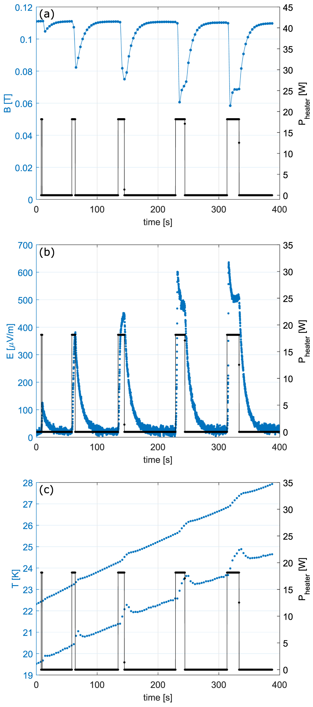
With the magnet operating at 4.4 kA in  K helium vapour, heat pulses with a maximum power of 18 W corresponding to a power density of 80 W cm−2 were applied using a thin-film heater shown in figure 1(b). During the heating pulses, the current in the magnet was kept constant and we simultaneously measured the magnetic field, voltage across the 4 middle turns, and temperature on the top and bottom of one current lead. At a heating power of 7.1 W, a local loss of superconductivity was observed. The heating power was increased to 18 W and the corresponding simultaneous response of voltage, magnetic field and temperature at the top and bottom of the current-leads as function of time for 5 heating pulses is shown in figure 10.

Figure 10. The measured development of the central magnetic field (a), the electric field across the 4 central turns of the magnet (b) and the temperature increase at the bottom and top of the coil (c) when turning on and off the quench initiate heater at a magnet operating current of 4.4 kA.
Download figure:
Standard image High-resolution imageIn figure 10 the pulse lengths, depicted by the black lines, were 2 s, 5 s, 10 s, 15 s, and 20 s. For each 18 W heating pulse, we observed a drop in magnetic field and development of voltage indicating loss of superconductivity. After the heater was switched off, the magnetic field recovered to the original value and the voltage disappeared. For the 2 s, 5 s, and 10 s pulses, the voltage was continuously increasing, and the magnetic field was continuously dropping over the entire heating period. The heat load into the magnet by previous pulses may have influenced the response to the following since the time to homogenise in between pulses was short. For the 15 s and 20 s pulses, which were performed at higher temperature, the magnetic field first dropped and then stabilised while the heater was on. This means that the magnet was partly still superconducting and current flowed partly helical. Also, for both pulses the voltage peaked and subsequently stabilised at a non-zero value. The peak may arise from the induced voltage by the dropping magnetic field and may cease by current-distribution.
When analysing data from the individual voltage-taps, corresponding to information across each half-turn, we observed that the quench spreads axially. Sections of the helix on the opposite side of the heater were found to be fully superconducting. After locally losing superconductivity, the current flows via the stabiliser and shorts, back to the tapes.
Over the course of the experiment, while the heater was switched off, the temperature at the top and bottom of the current leads, hence the temperature of the magnet since these are in thermal contact, increased steadily. The effect of switching on the heater on the temperature on the top and bottom of the current lead can be directly observed by the temperature sensors, as shown in figure 10(c). The effect of the heating pulses at the bottom sensor is larger as this sensor is mounted closer to the heater. Even though heat conduction and current redistribution to the copper current leads will have influenced the transient behaviour of the magnet, the stabilisation of magnetic field and voltage combined with measured superconductivity in sections of the coil shows that the self-protection by partial insulation and aluminium stabilisation works for this demonstrator magnet.
5. Model for simulating the performance of the magnet
A numerical model has been developed to study the transient behaviour of partially insulated high-temperature superconducting magnets and made public for everyone to use [18]. Below, we shortly describe the main working principles of the code. An elaborate description of the development of the code can be found in [19].
5.1. Setup of the numerical model
The code in its current form uses the geometry, materials, and conductor of the HTS coil described in section 2 as inputs, but it is written such that the geometry, conductor and material can be changed to any solenoid, stabiliser metal and ReBCO tape, respectively.
The model consists of coupled electric, magnetic and thermal parts. The electro-magnetic part is based on Kirchhoff's circuit laws and Biot–Savart law. The thermal part is a nearest neighbour model. After each electrical time-step, multiple, shorter thermal time-steps are performed to even out the nearest neighbour information.
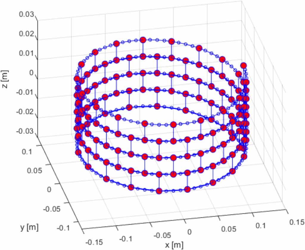
The code forms a model of the solenoid in the form of a helical-shaped nodal network, depicted in figure 11. Each node is connected to the next by a line element, in which current and heat can flow. Certain nodes are connected axially by line elements, representing partial insulation.
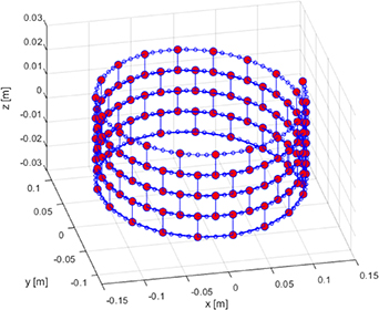
Figure 11. Nodal network used in the simulation. Line elements are visualised as blue lines and nodes as transparent or red dots. Red nodes are connected axially and helical, blue dots only helical.
Download figure:
Standard image High-resolution imageEach element has an electrical and thermal resistance dependent on temperature and an inductance. Helical elements are given a temperature dependent heat capacity, however the heat capacity of axial elements is considered negligible. Therefore, axial line elements do not have a temperature themselves and their material properties are calculated using an average of the two nearest helical line elements they connect.
For the electrical part, the self and mutual inductance of all elements are stored in a square symmetric matrix L, listing the self-inductance of each element along the main diagonal and the mutual inductance between element i and j in the off-diagonal elements.
The self-inductance of each line element, representing a section of the HTS cable or axial short, is approximated as the self-inductance of a long conductor of rectangular cross section (equation (24) in [20]) and is stored in matrix  , where i = j. The mutual inductance between line-elements i and j is calculated by a discretised version of the double integral Neumann formula [21] and is stored in
  , where i ≠ j:
The magnetic field at any point in space can be calculated using Biot-Savart Law
where  , the amount of current in each line element is considered constant across the line element and taken out of the integral.
The resistance of each line element is dependent on temperature T, and is calculated using the measured resistivity data for Al10SiMg depicted in figure 3 and coil geometry described in table 1. The voltage developed across each line element depends on the critical current of the superconductor  and
and  . The resistive current in each element is calculated using a critical state model assumption:

The dependence of the critical current on temperature T, magnitude of the local magnetic field B and angle of the local magnetic field with respect to the c-axis of the ReBCO crystal θB
is implemented in the code by the parametrised critical current density  fitted to the Fujikura FESC-SCH04 tape dataset [17] (see
Kirchhoff's laws are implemented using matrix M, comprising inductance and node and line-element connectivity information. It is generated once at the start of the simulation
where  and KV together ensure Kirchhoff's voltage law for each line element by adding the voltage of its neighbouring nodes, KV consists of zeros and ones and KI describes the ingoing and outgoing current at each node. By symmetry, KV and KI are each other transpose. O is a null matrix.
A set of equations is set-up in the form of

where  consists of
  at each line element, followed by the node voltage, and
  lists respectively the resistive voltage drop across each line element followed by
  flowing in and out each node.
The multiplication of the top section of M with 

denotes the implementation of Kirchhoff's voltage law: the voltage at each node is the voltage drop across the adjacent line element added up to the voltage at the adjacent node. The last node is grounded.
If we multiply the bottom section of M with  it follows that
hence the sum of  and thus the sum of I flowing in and out of each node is forced to be zero, Kirchhoff's current law.
Since we know the resistance of each element and  at each node
  (
( if we do not ramp the magnet up/down), and we want to know
  , and thus I in each line-element and the voltage at each node, which are contained in
  , we rewrite equation (9) as

For numerical efficiency, only the top half of this system of equations is solved for  at each element using MATLAB's ode15s solver for stiff equations.
Subsequently, the resistive voltage drop in  is calculated using updated current after each electric time step
  defined as
To conclude the electrical time step, the voltage at each node with respect to the last node is found using equation (12).
Each temperature step the change in temperature of helical line elements due to Joule heating  , heat conduction from to and from the neighbouring elements
  and any additional cooling
  or heating
  is calculated as
where Cp is the heat capacity of the element, approximated with the specific heat dependency on temperature of Al5083 from [23]. To determine the temperature at each line-element, equation (14) is integrated each temperature time step similar to equation (13).
5.2. Simulating the transient measurement conditions
The configuration of the ring shaped current leads has an effect on the transient behaviour of the magnet. Essentially, every point of the first and last turn are shorted to any other point of the respective turn by the high conductivity OFE copper ring. This effect is implemented in the model by setting the stabiliser resistance of each element in the first and last turn to that of the adjacent part of the copper ring, as the resistance of the ring is always lower than the resistance of Al10SiMg. Additionally, due to the high thermal mass of the current lead and the soldered connection, the current-leads act as a heat sink. This is modelled by adding a thermal link from each element of the first and last turn to an edge element at the respective edge with the heat capacity of that current-lead. This way, heat can flow to and from the rings, and the temperature profile along the rings is considered uniform, as the thermal conductivity of OFE copper is high.
Since the magnet was cooled by helium vapour during the measurement, convection cooling by the vapour was implemented in the simulation code and estimated using the Nusselt number. In the simulations, we set the gaseous helium to have a constant temperature of 20 K. The helium convection heat flux term in equation (14) is implemented as:
where  is the thermal conductivity of helium at 20 K and 0.01 MPa [24],
  denotes the temperature gradient between the element and the helium gas, w is the characteristic length scale, here chosen as the average width of the element, Nu is set to 4.36 under the assumptions of a fully developed laminar circular tube flow with uniform surface heat flux [25], and A is the exposed surface area of the line element.
6. Comparison of the simulation and experiment
We simulated the transient behaviour of the coil with the model described in section 5. The timing and power of the heating pulses is replicated in the model by setting  in equation (14) to the measured value for the time it was switched on. The simulated response of the central magnetic field, electric field over the middle 5 turns, and temperature at one current lead of the magnet to heating pulses are displayed in figure 12, respectively. The magnetic field drops as the heater is switched on, and recovers when the heater is turned off. Simultaneously, an electric field develops and fades. In the simulation, the field drops more than in the measurement.

Figure 12. The simulated development of the central magnetic field (a), the electric field across the 4 central turns of the magnet (b) and the temperature at one current lead (c) when turning on and off the quench initiate heater at a magnet operating current of 4.4 kA.
Download figure:
Standard image High-resolution image
In the measurement, the magnetic field and electric field reach a stable value for the 15 s and 20 s heating pulse. However, in the simulation, these do not stabilise. The simulated peak electric field is roughly a factor two smaller than measured for each heating pulse. The video included as supplementary material of this paper shows the current and critical current distribution along the helix of the magnet as function of time and the heating pulses.
The video shows that the quench spreads axially. The coil is heated in the middle line element where the local Ic decreases. Once the local Ic is lower than the current in the element, the current starts to take the axial line elements to the adjacent turns. However, the heat propagates concurrently via the axial line elements, decreasing the local Ic at the next turn causing the current to redistribute again. The Ic in the outer turns does not decrease as fast, as the heating in that turns is lower, since they are connected to a copper current lead. It takes most current and maintains part of the magnetic field.
The time constant of recovery is slower in the simulation than in the measurement. As can be seen in the video, the recovery time constant in the simulation is mainly dominated by the recovery of  . When recovering, the elements do not take more current than
  .
.
Both in the simulation and measurement a similar delay in the peak and decrease of temperature of the current-lead can be seen after the heater was turned off.
The results from an axi-symmetric COMSOL simulation of the central magnetic field and inductance across 4 turns shown in figure 2 are compared in table 2 to the measured values. The difference between the compared values is around 1%.
Table 2. Comparison of simulated and measured values of the central magnetic field at ( A), and inductance of the four central turns of the HTS magnet. Uncertainties are given at 2σ level.
| Measured | Simulated | Difference | |
|---|---|---|---|
| Central B-field |
 T T | 0.114 T | 0.9% |
| Inductance |
 µH
µH | 7.3 µH | 0% |
7. Discussion
7.1. Experimental part
Currently, 3D-printing limits the size of the coil to approximately 500 mm diameter open bore. Metal printing technology is developing fast so it might be possible in the future to print larger geometries.
No tension could be applied while winding the tapes to the inside of the cylinder. Although soldering the tapes to the external surface of the cylinder could alleviate this challenge, it was decided to solder them to the inside of the cylinder due to the structural support the cylinder can offer against the Lorentz forces acting on the tapes. While this approach may seem unnecessary for a small prototype from a mechanical perspective, it closely mirrors the requirements of supporting tapes for full-scale detector magnets, making it a design choice that aligns with the final intended application.
In the HTS magnet developed in this work, the stack of ReBCO tapes is positioned in a staircase pattern near the junctions with the Hastelloy layer pointed away from the aluminium. Each tape end has a 4 mm × 20 mm direct contact with the coated aluminium lowering the contact resistance to each ReBCO layer. This configuration is mechanically weaker than if the tapes would be soldered facing the Hastelloy to the aluminium. If a coil with higher fields would be built, this should be taken into account. In our case, this was not needed so we opted for a lower contact resistance.
The soldering process for future coils could be improved by soldering a stack of tapes together before soldering to the cylinder to prevent tapes slides during the process. However, dedicated machinery would be needed. Also, soldering in a vacuum oven may decrease the number of voids in the joint.
From the shape of the current-to-electric field measurement across 4 turns at 77 K in figure 7 one can observe that around 580 A the magnetic field does not increase linearly with the current anymore. The  limit of the tapes is at least locally reached and the current redistributes. The field flattens of as more current flows axially via the shorts. Following the convention, the power-law (
 ) was fitted to find
  where E0 is 100 µV m−1. The power-law however empirically describes superconductors, not stabilised cables, and it is important to note that the fit gives an artificially low n-value since the practically linear slope of E-field above 580 A in this case essentially corresponds to the stabiliser resistivity.
7.2. Numerical part
The code uses the critical state model meaning that all current of each line element above Ic
is carried by the stabilising metal. Implementing a power-law model will make the simulation more similar to the real behaviour, where the superconductor can take more current than Ic
. However, implementing the critical state model gives the 'worst case scenario' and therefore a conservative estimation of the quench behaviour, which is desired given that large-scale detector magnets are generally designed to have large  margins of a few 10%.
The parameterisation of the Fujikura ReBCO tape data set describes the critical current reasonably well (around ±10%) up to 40 K. Above 40 K, the parameterised critical currents deviate  10% from measured values and the deviations get worse with higher temperatures and higher magnetic flux densities. As the hot spot temperature of the coil rose up to ∼100 K, this will have an effect on the accuracy of the model.
The initial temperature profile of the coil is set to 20 K, and the temperature of the helium gas is kept constant at 20 K for simplicity. In the measurement, there was a temperature gradient in the coil as described by equation (3) and in the helium gas. As Ic depends on temperature, this may have an effect on the transient behaviour of the magnet. The heater is attached to the bottom of the coil, where the temperature is the lowest, and as most of the transient effect take place in that location we took the initial temperature of the bottom of the current lead as the initial temperature of the coil in the model. We deem this estimation to accurately describe the region of interest.
The low E-field in figure 10(a) is party explained by how the two copper rings were implemented; we set the first and last turns to have the electrical resistance of OFE copper to keep the overall simulated geometry simple and general. The resistivity of OFE copper is several orders of magnitude lower than that of Al10SiMg. Therefore, the resistance of the aluminium stabiliser in the outermost two turns is not taken into account, explaining part of the discrepancy between the simulated and measured voltages in a transient. This could be improved by adding line-elements describing the current leads and the connection from the helix to the copper current leads. In addition, the resistivity of tin-lead solder and the copper stabiliser of the tapes is not taken into account, further reducing the developed voltage in practise.
The discrepancy between the simulated and measured temperature of the current lead results from several factors. These include assumptions in the cooling model, imperfect thermal contact of the sensors, lower voltage in model leading to reduced heating, and in practice, the current leads being in contact with busbars that slowly heat up due to resistive current. These real-world conditions can significantly impact the temperature profile but are not accounted for in the model.
In the future, the simulation code could be extended by including a ramping option and by adding connected parallel line elements to every helical line element to simulate eddy currents. Also, the effect of the current-lead on transient effects can be replicated more accurately by adding line-elements to resemble the current leads instead of changing the resistance of the existing line elements of the first and last turn.
7.3. General
In the future, this type of magnet could be operated with cryocoolers. Two cryocoolers can have a combined cooling-power at 4.2 K of 4 W which is sufficient in terms of heat load. The cooling power of cryocoolers increases significantly with temperature, for example for two cryocoolers of a certain type the combined cooling power increases to 40 W at 30 K [26]. For a future larger HTS demonstrator coil, the joint resistance and heating of the magnet may be minimised by soldering the HTS tapes directly to the copper current leads. Soldering more tapes to the cylinder will allow operation at the same current at elevated temperatures, and thus increased cooling efficiency.
The stability of the HTS magnet during local heat pulses is a result of a combination of aluminium stabilisation, partial insulation and the copper current leads acting as heat sinks and conductor. However, based on the similar simulation conditions but without the copper current leads, we noted that the hot spot temperature would not exceed 120 K as there is heat conduction both via helical and axial shorts.
8. Conclusion
We have successfully built, modelled and tested an aluminium-stabilised, partially insulated and thereby self-protected HTS demonstrator magnet. The manufacturing process is explained, it is shown that ReBCO tapes can be soldered to electrochemically coated aluminium without observable degradation, the performance of the magnet is experimentally tested and the critical current is obtained from 30 K to 77 K. Due to the low contact resistance to the current leads, the magnet is compatible to operate with cryocoolers in terms of heat-load. The magnet operated stably in helium vapour for over an hour at 4.4 kA, which was the maximum current of our power supply, and proved to be stable when superconductivity was broken locally using a thin-film heater. Even though voids in the soldering joint were observed, no degradation was observed after 12 thermal cycles and locally quenching the magnet. It is promising that this technology works, in spite of imperfect soldering quality. Improving the manufacturing quality leaves margin for further enhancing the performance of aluminium stabilised HTS conductors.
The developed numerical model for simulating transient behaviour of partially insulated HTS coils is verified against measurements and provides insight in how current redistributes when such coil locally loses superconductivity. The simulated and measured developed electric field and magnetic field drop when locally breaking superconductivity differ at most a factor two.
The shown thermal and electrical stability of the HTS demonstrator coil during a local quench combined with the usage of high resistivity aluminium as a stabiliser serve to illustrate the main conclusions of this paper: aluminium alloys are a good candidate for stabilisation of HTS-based detector magnets and quench protection by partial insulation is suitable for this type of magnet. CERN EP R&D programme continues in developing and scaling up this technology.
Acknowledgments
The authors thank Dr Tim Mulder from CERN for useful discussions on quench simulations of partially-insulated HTS magnets, Dr Davide Uglietti from PSI for solder coating our ReBCO tapes, and Mr Michal Dalemir Celuch from CERN for performing a 3D-computed tomography scan of the HTS magnet. This work was supported by CERN EP R&D on Experimental Technologies (WP8 Detector Magnets).
Data availability statement
All data that support the findings of this study are included within the article (and any supplementary files).
Appendix: Equations used for critical current density fitting
The equations to parametrise  of the HTS tapes used in this work are listed below. The fitted parameter values obtained are provided in table 3,

Table 3. The fitted parameter values for Fujikura FESC-SCH04 tape.
| Function | Parameter | Fitted value | Unit |
|---|---|---|---|

| g0 | 0.041 63 | dimensionless |
| g1 | 0.371 11 | dimensionless | |
| g2 | 0.037 44 | dimensionless | |
| g3 | 0.061 46 | dimensionless | |

|

| 11.76 376 | A mm−2 |

| 30.068 41 | K | |

| 0.166 64 | T | |
| m1 | 0.235 34 | dimensionless | |
| n1 | 1.357 55 | dimensionless | |

|

| 3.386 56 | A mm−2 |
| Tab | 36.036 86 | K | |
| Bab | 0.992 35 | T | |
| c | 1.885 78 | dimensionless | |
| n2 | 1.633 30 | dimensionless | |
| h | −0.006 44 | dimensionless | |
| p | −0.175 04 | dimensionless | |

| 8.111 90 | K | |

| γ | 1.845 77 | dimensionless |
| s | 0.006 98 | A mm−2. |

Supplementary data (3.9 MB MP4) Simulated time evolution of current distribution along helix when locally quenching the coil.