

Abstract
In this paper, we extend some recent works about the Doppler effect in surface waves on water. We improve the experimental set up by exploring several situations: source in motion with constant velocity and receiver at rest, source at rest and receiver in motion with constant velocity, as well as both source and receiver in motion. Thereby we produce fractional frequency changes  of the order of 40%–50%, far larger than those obtained by more traditional sound experiments. The experimental setup, the data collection and the data analysis also allow to highlight some aspects relevant from a didactic point of view, in particular, the experimental results clearly show the nonlinearity of the Doppler shift with the moving source velocity.
Export citation and abstract BibTeX RIS

Original content from this work may be used under the terms of the Creative Commons Attribution 4.0 licence. Any further distribution of this work must maintain attribution to the author(s) and the title of the work, journal citation and DOI.
1. Introduction
The Doppler effect has always been a highly intriguing phenomenon for students and a source of teachers' inspiration for constantly renewed educational proposals. Recently, for example, the use of devices closer to students' experience (smartphones) and more powerful and versatile tools for analyzing video recordings (Tracker), has been the recurring focus of several publications devoted to the acoustic Doppler effect (see for example [1–4] and the references therein). Still in connection with the use of new technologies, starting from a work by Serra [5], other recent papers studied the Doppler shift with plane surface waves on water [6, 7]. In particular, thanks to the use of on-line probes and a plotter, in order to produce displacements with constant speeds, the experiments in [6] about a source at rest and a moving observer showed fractional frequency changes
 as high as 40%–50%, while a general algebraic and graphical approach suitable for high school students was developed.
Considering again surface waves on water but using instrumentation slightly expanded from that employed in [6], in this paper we present quantitative experiments with the moving source. In the first set of situations, the receiver is kept at rest, while later situations where both source and receiver move are examined. We believe that this proposal could be of educational interest since to our knowledge most of the activities offered in school are qualitative or limited to situations where the fractional frequency change  turns out to be quite small (a few % only) preventing the possibility to observe its nonlinearity with the source velocity.
The paper is organized as follows: section 2 describes the equipment used in the various situations, and section 3 shows how the propagation speed of the surface wave is determined. In section 4, starting from a general result for frequency fractional change (Doppler shift) presented in [6], formal tools for comparison with experimental results are developed. Section 5 describes and presents the results of the experiments with the source in motion and the receiver at rest, while section 6 considers situations in which both the source and receiver are in motion. Finally, section 7 summarizes the results and outlines some possible developments from an educational perspective.
2. The experimental setup
Figure 1(a) presents the essential elements of the setup. Figure 1(b) gives the overall scheme (top and side view). The ripple tank (Leybold Wave Trough 401 501) is filled with 500 mL of water, resulting in a layer that is about 6.5 mm deep. The easiest way to study cases with the source in motion is to use circular wavefronts generated by an air outlet nozzle, connected to the air pulse generator with a flexible silicone hose and mounted on a motorized cart (Pasco Wireless Smart Cart ME-1241 equipped with Smart Cart Motor ME-1247). The cart moves at a speed between 3.5 and 12 cm s−1 (determined for each run through the cart's wireless connection), along a horizontal track (Pasco 1.2 m Aluminum Dynamics Track ME-9493), located alongside of the ripple tank and at a suitable height for the nozzle to generate well-defined wavefronts. The image of the waves on the translucent vertical screen, obtained with the lighting system of the tank, allows for an overall view of the source/receiver motion.

Figure 1. Image (a) and schematic (b) of the equipment used: the source is mounted on a cart equipped with a motor, while the light sensor travels solidly with the plotter arm. Note that the speed of the (virtual image of the) receiver is different from that of the light sensor.
Download figure:
Standard image High-resolution imageAfter removing the vertical translucent screen, the time evolution of the luminosity at a given point is detected by a light receiver (Pasco High Sensitivity Light sensor PS-2176), mounted on the moving arm of a plotter (Goertz Metrawatt BBC Servogor SE 790) available in our school (otherwise, a second motorized cart can be used). In separated tests we assessed the actual values of the three velocities of the plotter arm: 1.97 ± 0.03 cm s−1, 4.93 ± 0.06 cm s−1 and 9.87 ± 0.10 cm s−1.
The position of the light sensor identifies on the water surface the point where the (virtual image of the) receiver is located (see figure 1(b)). Because of the divergence of the light beam used for projection, the displacement of the (virtual) receiver is proportional to that of the light sensor by a magnification factor A = 2.28 ± 0.05. The latter is determined as the inverse ratio between the actual sizes of objects placed in the ripple tank and the sizes of their projected shadows, and it is found to be almost constant in all positions. The velocities of the (virtual) receiver turn out to be 0.864 ± 0.020 cm s−1, 2.16 ± 0.05 cm s−1 and 4.33 ± 0.10 cm s−1 respectively.
The equipment must be aligned accurately so that the position of the (virtual) receiver remains consistently along the direction of movement of the source. Thus, while using circular wavefronts, the 'simplified' formalization valid for the one-dimensional case can be still used (see section 4). In addition, to prevent the light sensor from being disturbed by the shadow produced by the nozzle air holder, the latter is positioned transversally to the direction of the source motion.
All data collected from the sensors are stored and processed with the Capstone software version 2.5 (https://www.pasco.com/products/software/capstone).
Differently to what is presented in [6], the lamp intensity of the ripple tank available oscillates with a frequency of 100 Hz. Unfortunately, this leads to an effect on the intensity measured by the light sensor, since this frequency overlaps with that of the source. To overcome this, we operated the halogen lamp of the light source with an external stabilized power supply.
To effectively use this experiment in the classroom, it is helpful—after repositioning the translucent screen of the ripple tank—to replace the light sensor with a video camera, possibly connected to a beamer.
3. Measurement of the wave velocity
In order to make a comparison between the measured frequencies and those computed on the basis of the adopted theoretical model, it is necessary to know the value of the velocity of the water surface waves (c). For this purpose, we performed a specific experiment using two light sensors placed side by side. After finding a reference situation by which their signals are in phase, one of them is repeatedly shifted by 5 mm measure after measure. From the data collected with the two sensors (each operating with a sampling rate of 1 kHz), the time delay Δt, i.e. the delay accumulated by one relative to the other, is determined for each total displacement Δx. Since the procedure is quite similar to that described in [6], for brevity, here we limit ourselves to report the experimental results (see figure 2).

Figure 2. Wavefront displacement versus time delay (with a water layer of 6.6 ± 0.2 mm depth): from the slope we get a propagation velocity of c = 22.55 ± 0.25 cm s−1.
Download figure:
Standard image High-resolution imageA linear trend is observed. The slope allows to determine the velocity c of surface waves: since the wavefront advancement is obtained as the ratio of the displacement Δx of the sensor to the geometric magnification factor A, we obtain c = 22.55 ± 0.25 cm s−1 (See the supplementary materials for further details of the experiment).
Performing the entire set of measurements takes several hours. Therefore, we found necessary to check whether the inevitable evaporation of water leads to significant changes. For this purpose, we repeated the measurement of the wave velocity with a slightly thinner water layer (450 ml in the ripple tank, for a thickness h of about 6.0 mm) obtaining almost the same result. These values are in agreement with Kelvin's law [5] for surface waves on water (with λ ≈ 2 cm), both for the value obtained for the velocity, as well as for its very weak dependence on depth in situations where  is close to its asymptotic value.
4. Theory and parametrisation of the various experimental situations
A general expression for the value of the Doppler shift in the most general case has been the object of several papers. All these studies have pointed out that besides the purely kinematic aspects concerning the source and the receiver, and the specific shape of the wavefronts, also the time delay due to the finite propagation velocity of the perturbation must be taken into account (for example see [8, 9]). In our experiments, the position of the (virtual) receiver is always kept as best as possible along the line of motion of the source, both when it is at rest and when it is moving. In this way, even employing a 'point source' (and thus dealing with circular wavefronts) the situation can be considered one-dimensional. Nevertheless, even in this simplified situation, the number of possible cases and sub-cases is still quite large. The use of vector notation—as suggested in [6, 10]—enables the formalism to be compacted. For the Doppler effect involving acoustical and surface waves one can indeed write:

where  is the (proper) frequency of the source,
  is the frequency perceived by the receiver,
  is the velocity of the source,
  is the velocity of the receiver and
  is the velocity of the wavefront (where all three velocities are understood to refer to the medium of propagation). Notice that in equation (1) there is no explicit time dependence of the various quantities. This implies not only that we are limited to situations in which the absolute value of the various velocities involved remains constant, but also that even in our one-dimensional case the direction of the various vectors must be carefully considered. We will do this by introducing the angles
  (between the forward direction of the source motion and that of the wavefront) and
  (between the forward direction of the receiver motion and that of the wavefront perceived by the receiver). Furthermore, since the source can be either at the right or at the left of the receiver (and move towards or away from it in both situations), to consider all the possible various cases, it is useful to make them graphically explicit.
Observing that under the conditions of one-dimensional geometry described above, the angles  and
and  can assume—independently from each other—only the values 0 or
  we derive from (1) the following expression for the frequency fractional change:

where the symbol employed for each velocity represents its respective absolute value. Equation (2) can be consequently rewritten as:

We are faced with eight cases: four with the source moving to the right, four with the source moving to the left. Assuming isotropy in wave propagation, by symmetry the latter can be traced back (algebraically) to the four cases with the source moving to the right. They are depicted in figure 3.

Figure 3. Schematic diagram of possible situations: the 4 cases with the source moving to the right are shown. By symmetry, the 4 cases with the source moving to the left can be traced back to these.
Download figure:
Standard image High-resolution imageIn all our experiments the source moves with a velocity less than that of the wave ( ): the inequalities shown in figure 3 for cases (a) and (c) refer to this situation. In configurations of type (b) there is a decrease of the perceived frequency, in configurations of type (c) an increase. In configurations (a) and (d), in which the two terms in the numerator have opposite signs, both situations are possible.
5. Moving source and receiver at rest: measuring the Doppler shift
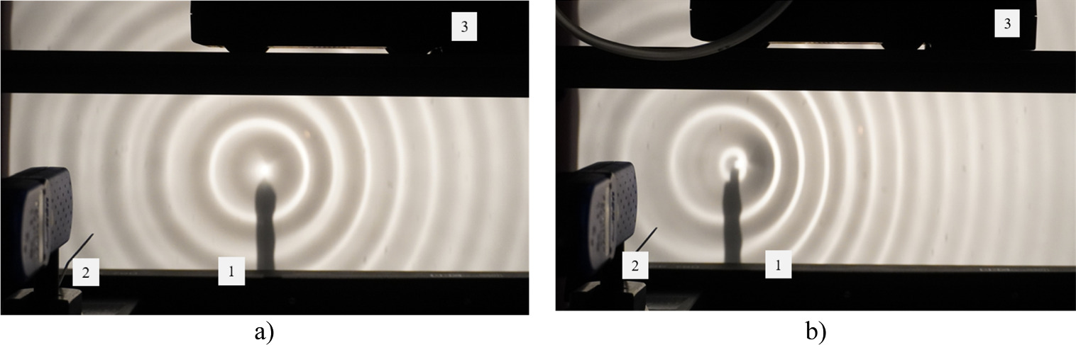
The experiment is carried out by letting the source (i.e. the motorized cart on which it is mounted) move to the right at a constant velocity. Figure 4 shows a typical image of what can be observed on the translucent screen: initially the source lies to the left of the receiver, and we expect that a receiver that is to the right of the source (i.e. when the source is approaching it—case (a) in figure 3, with  ) will perceive an increased frequency, while a receiver that is to the left of the source (i.e. when the source is moving away from it—case (b) in figure 3, with
  ) will perceive a decreased frequency.

Figure 4. Doppler effect generated by a moving source (to the right) on the water surface inside the ripple tank: (a) υs = 3 cm s−1; (b) υs = 7 cm s−1. In addition to the shadow of the source holder (1), the light sensor (2) mounted on the plotter arm (bottom), as well as a partial silhouette of the motorized cart (3) are distinguishable. Videos are available in the supplementary materials of the online edition.
Download figure:
Standard image High-resolution imageFigure 5(a) shows a typical example of a dataset obtained for the source velocity, while figure 5(b) shows the associated light intensity recorded by the light sensor.

Figure 5. Typical measured dataset: (a) source velocity (sampling rate 50 Hz): average value is used for data analysis ; (b) light intensity recorded by the light sensor (sampling rate 1 kHz). The change in the peaks period between phase I (0.65–2.35 s, approaching) and phase II (receding) is clearly visible.
Download figure:
Standard image High-resolution imageIn order to determine the frequency at which the light sensor receives the various light peaks in the approaching phase and in the receding one, we first identify on the graph the arrival times of the various peaks (numbering them progressively). Then we represent those values as a function of the peak number. Figure 6(a) illustrates the results obtained with the source at rest. It allows us to determine the value of the proper frequency of the source: the inverse of the slope value gives f0 = 12.14 ± 0.15 Hz. Figure 6(b) refers to the situation in which the source travels with a constant velocity of vs = 6.11 ± 0.15 cm s−1. The phase in which it approaches the receiver and that in which it moves away from the receiver are clearly distinguishable. A linear trend is observed for each of them: again, the slope value gives us the period of the incoming signal, and its inverse the corresponding frequency (see table 1).
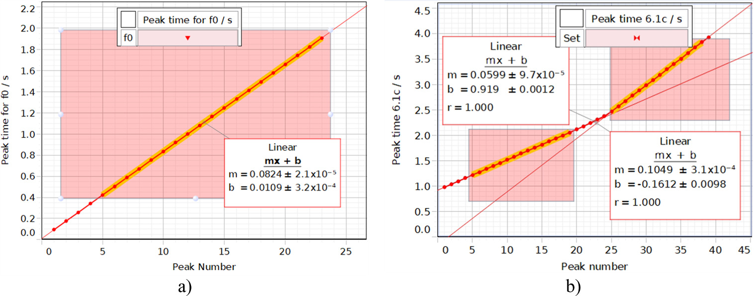
Figure 6. Typical experimental results for determining the period recorded by the receiver when the source velocity is: (a) υs = 0 cm s−1; (b) υs = 6.11 ± 0.15 cm s−1 (numerical values from the data in figure 5(b)).
Download figure:
Standard image High-resolution imageThe experiment was repeated several times for each of the cart velocities. Table 1 summarizes the results obtained as well as the values calculated from equation (3) assuming for the velocity of the surface waves the value c = 22.55 ± 0.25 cm s−1.
Table 1. Frequency fractional change: comparison of the values obtained from frequency measurement and from velocity measurement. The detailed analysis of each run is available in the supplementary materials of the online edition.
|
The uncertainties in table 1, as those in all the other ones or in the graphs, are determined not so much on the basis of the statistical analysis of each single run, but rather by taking into account the fluctuations observed both within and between similar runs. For example, the uncertainty on the cart velocity was established considering its very difficult reproducibility, mainly caused by the presence of the hose.
Using  to parameterize the motion of the source, it is possible to conveniently discriminate between the phase during which the source is approaching the receiver (case a in figure 3, with
  ) respectively that during which the source is receding from the receiver (case d in figure 3, with
  ).
).
The experimental results are shown in figure 7 (red points), together with the theoretical trend predicted by equation (3) (black line):

Figure 7. Frequency fractional change versus source velocity: measured values (red dots) and expected theoretical predictions (black line).
Download figure:
Standard image High-resolution imageThe very good agreement observed justifies a posteriori the model adopted, in which have been neglected both the unavoidable presence of reflected waves with slightly different frequencies (leading to a distortion of the peaks), as well as the possible change in the maximum intensity conditions in the light projection, due to the dispersive phenomena affecting the surface waves on water.
These first results show very clearly how the proposed experiment with the moving source, even in the case in which the receiver is at rest, allows to highlight the nonlinear dependence of the Doppler shift on the source velocity.
This issue is unavoidably neglected in the investigations involving the acoustic version of the experiment [1–4] where it could be even explicitly contradicted by highlighting symmetries between the approaching and receding phases, without specifying that they are valid only approximately and in a very limited range of velocities (for example [4] p. 567).
6. Moving both source and receiver
The configurations in which both source and receiver are in motion, are still those of figure 3. However, depending on the velocities involved, in (a) and (d) the distance between source and receiver can increase or decrease, so that if  the value of
  can be both positive (source and receiver are approaching) or negative (are moving apart).
Therefore, great care must be taken in the analysis of the various configurations. In particular, it must be remembered that the speed of the (virtual) receiver is related to the speed of the sensor (fixed by the plotter controls, in our experiment) through the magnification factor. In order to illustrate how much situations can get fuzzy, in figure 8 we analyze a run in which the light sensor is kept moving to the right with a constant velocity of 1.97 ± 0.03 cm s−1 (i.e. a (virtual) receiver velocity of 0.86 ± 0.04 cm s−1), while the source, initially at rest on the left of the receiver (phase I), is then set in motion with a speed of about 6.5 cm s−1 in the same direction. This way, it next pursues and reaches the receiver (II), overtakes it (III) and finally stops to its right (IV). For each of the four phases, in figure 8 the kinematic diagram is shown, as well as the algebraic relationship needed to determine theoretically the frequency perceived by the receiver and the subsequently frequency fractional change. It is interesting to notice how the distance between source and receiver increases in phases I and III, decreases in phases II and IV.

Figure 8. Light intensity recorded by the receiver versus time. The receiver is kept moving to the right with constant velocity, while the source, initially at rest to its left (phase I), reaches it (phase II), overtakes and distances it (phase III), and finally stops and remains at rest to its right (phase IV).
Download figure:
Standard image High-resolution imageThe data analysis is that of the previous section. In order to obtain reliable numerical values, the wave velocity and the frequency should be preliminarily checked: we obtain c = 22.55 ± 0.15 cm s−1 and f0 =12.14 ± 0.15 Hz (for details, see supplementary materials). Next, the source velocity is determined: as shown in figure 9, its (average) velocity changes slightly in the second part of the path (probably due to the way the hose supplying the air nozzle was supported by hand) increasing from 6.39 ± 0.20 cm s−1 to 6.59 ± 0.20 cm s−1.
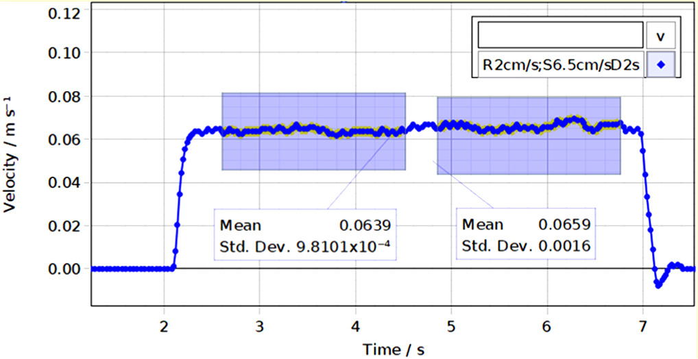
Figure 9. Determination of source velocity: it can be seen that the velocity does not remain exactly constant: in the second part of the run (phases III and IV) it is somewhat higher than at the beginning (phases I and II).
Download figure:
Standard image High-resolution imageThe next step is to determine the frequencies perceived in the different phases. In figure 10 the instants of arrival of the different peaks are represented as a function of the progressive number with which they appear in figure 8. This way, it is possible to assign to each of the four phases described above the slope of a sufficiently linear trend, corresponding to the period of the signal recorded by the receiver, and then the relative frequency.
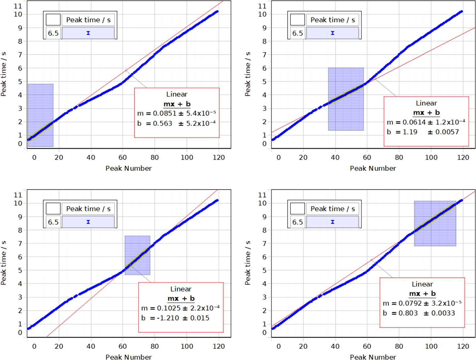
Figure 10. Determination of the frequency of the received signal for the various phases.
Download figure:
Standard image High-resolution imageWe now have all the information necessary to determine, as showed in table 2, the frequency fractional change  and to compare it with the corresponding theoretical value computed through the source and receiver velocities, according to relation (3) (see table 2).
Table 2. Comparison of measured and calculated values.
|
Overall, a fair agreement is observed. As can be expected, also taking into account the uncertainties associated to both frequency f0 and propagation velocity c, the situations with a small Doppler shift (i.e. with the source at rest) are those with the highest discrepancy.
It may be worth observing in detail the behavior at the transition from phase II to phase III, i.e. the moment in which the source overtakes the receiver, so that the direction of the incoming wavefront changes suddenly. Figure 11, in contrast with figure 7, shows that a moving receiver determines a splitting effect: the cases in which the source and receiver are approaching and those in which they are moving away lie on two different branches.
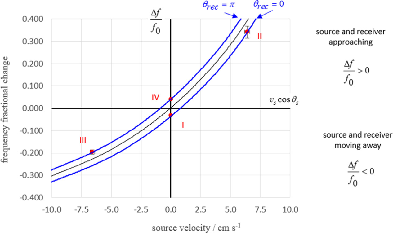
Figure 11. Detailed analysis of the run of figure 8: each of the four phases is represented by a point. The motion of the receiver (υrec = 0.864 cm s−1) determines the splitting into two branches: notice the 'jump' in the transition from phase II to phase III.
Download figure:
Standard image High-resolution imageFrom the experimental point of view, we observe that the 4 points fall with more than acceptable accuracy on the respective theoretical curves. Interestingly, at the moment when the source overtakes the receiver there is not only a sudden change in the sign of the term  but also a 'jump' of the respective configurations from one branch curve to the other, due to the transition from
  (phases I and II) to
  (phases III and IV).
With our experimental setup we tried to get a wide range of situations like this one, but after a few attempts we realized that it is quite difficult to obtain runs including more than one interesting configuration. There are principally three serious limits: (1) the plotter arm, i.e. the light sensor, can move only in one direction with fixed velocities (0.864 cm s−1, 2.16 cm s−1 and 4.33 cm s−1, for the (virtual) receiver); 2) with a second motorized cart, the first problem could be solved, but the minimum constant velocity of all these carts is about 3.5 cm s−1; 3) beside these technical aspects, the travel time of the wave determines a delay between the instant in which a kinematic change happens in the motion of the source and/or receiver, and that in which this change is actually noticed by the light sensor. This delay is difficult to manage operationally, because, in turn, it depends not only on the distance between source and receiver at a given time, but also on their velocities. Also for this reason, the runs with more than one useful configuration were those with the lowest receiver velocity.
We therefore opted for a series of runs in which we could realize only a single configuration, identifying for it the relevant phases (time intervals), accordingly to the data analysis procedure explained above. Figure 12 summarizes the experimental results obtained (detailed analysis for each individual configuration are available in the supplementary materials). Data are organized according to the receiver speed  and the angle

Figure 12. Frequency fractional change as a function of the source velocity: comparison between experimental results (full dots) and theoretical predictions (continuous lines) for three different values of receiver velocity (blue: υrec = 0.864 cm s−1; green: υrec = 2.16 cm s−1; red: υrec = 4.33 cm s−1).
Download figure:
Standard image High-resolution imageIt was possible to implement configurations for each of the four quadrants and for each of the four types (a–d) in figure 3. More specifically, for situations where source and receiver are approaching (i.e. when  in the first quadrant there are configurations of type (c) as well as configurations of type (a) with
  while in the second quadrant there are configurations of type (d) with
  For situations where source and receiver are moving apart (i.e. when
  ), in the third quadrant there are configurations of type (b) and configurations of type (d) with
  while in the fourth one, those of type (a) with
  Marginally let us point out that the six points along the y-axis coincides with the configurations depicted in figure 3 of [6], i.e. those associated with situations with source at rest
  and receiver in motion.
Figure 13 gives an overview of all the values obtained for the frequency fractional change  presenting a quite good agreement between those determined from the frequencies and those determined from the velocities.

Figure 13. Frequency fractional change determined from the measured frequencies and calculated from the velocities: black dots refer to situations with vrec = 0, blue dots to those with υrec = 0.864 cm s−1, green dots to those with υrec = 2.16 cm s−1, and finally red dots to those with υrec = 4.33 cm s−1. The dashed line indicates the theoretical prediction (bisector).
Download figure:
Standard image High-resolution image
7. Conclusion and outlook
In this paper, the experiment proposed in [6] using surface waves on water, has been extended, in particular to situations where the source is in motion. From the experimental point of view, we demonstrated the adequacy of the proposed setup in order to complete the quantitative exploration of the Doppler effect in cases where the presence of a material medium (in our case the water) defines a privileged reference frame relatively to which the wave possesses a well-defined velocity. In particular, with the setup presented in this paper it is possible to generate frequency fractional changes  of the order of 40%–50%, far superior to what can be achieved in the classroom with acoustic waves (including ultrasound). We also observe that this equipment could be deployed for the experimental study of situations where the source velocity is higher than the wave velocity.
From an educational point of view, the proposed experiments allow for dealing with situations in which both source and receiver are in motion. This is interesting from two different and complementary points of view. On one hand, they allow to link the Doppler effect to concrete domains of application such as astronomy: in fact, the relative radial velocity of stars in our galaxy is measured by the Doppler shift of the light frequencies contained in their spectra, and corrections taking into account the observer's velocity are necessary to refer the source velocity to the galactic center. On the other hand, the proposed experiments enable students to improve their understanding of the principle of relativity. This is not only outlining the reasons why–in the case of sound or surface waves on water—the differences between the situation with a source at rest and a moving receiver and that with a moving source and a receiver at rest do not constitute a violation of the principle of relativity. In fact, since light is involved in many Doppler effect applications (such as in astronomical determinations), there is also an opportunity to introduce students to situations in which the relative velocity of source and receiver turns out to be the uniquely relevant parameter, i.e. situations where there is no longer a preferred reference frame relatively to which the signal propagates at a well-defined velocity: this issue would be the focus of a forthcoming paper.
Acknowledgments
We would like to thank the Liceo di Bellinzona for kindly hosting and allowing the largely use of the equipment needed to carry out the experiments presented here. This work was supported by the Open Access Publishing Fund of the Free University of Bozen-Bolzano.
Data availability statement
All data that support the findings of this study are included within the article (and any supplementary files).
Supplementary data (3.2 MB PDF)
Supplementary data (1.5 MB PDF)
Supplementary data (6.4 MB PDF)
Supplementary data (0.5 MB JPG)
Supplementary data (0.7 MB JPG)
Supplementary data (1.9 MB PDF)
Supplementary data (0.9 MB MP4)
Supplementary data (2.3 MB MP4)
Supplementary data (1.3 MB MP4)
Supplementary data (1.3 MB MP4)