

Abstract
Recently, quantum neural networks or quantum–classical neural networks (qcNN) have been actively studied, as a possible alternative to the conventional classical neural network (cNN), but their practical and theoretically-guaranteed performance is still to be investigated. In contrast, cNNs and especially deep cNNs, have acquired several solid theoretical basis; one of those basis is the neural tangent kernel (NTK) theory, which can successfully explain the mechanism of various desirable properties of cNNs, particularly the global convergence in the training process. In this paper, we study a class of qcNN composed of a quantum data-encoder followed by a cNN. The quantum part is randomly initialized according to unitary 2-designs, which is an effective feature extraction process for quantum states, and the classical part is also randomly initialized according to Gaussian distributions; then, in the NTK regime where the number of nodes of the cNN becomes infinitely large, the output of the entire qcNN becomes a nonlinear function of the so-called projected quantum kernel. That is, the NTK theory is used to construct an effective quantum kernel, which is in general nontrivial to design. Moreover, NTK defined for the qcNN is identical to the covariance matrix of a Gaussian process, which allows us to analytically study the learning process. These properties are investigated in thorough numerical experiments; particularly, we demonstrate that the qcNN shows a clear advantage over fully classical NNs and qNNs for the problem of learning the quantum data-generating process.
Export citation and abstract BibTeX RIS

Original content from this work may be used under the terms of the Creative Commons Attribution 4.0 license. Any further distribution of this work must maintain attribution to the author(s) and the title of the work, journal citation and DOI.
1. Introduction
1.1. Background—quantum/classical neural networks and classical neural tangent kernel (NTK)
Quantum neural networks (qNNs) or quantum classical hybrid neural networks (qcNNs) are systems that, based on their rich expressibility in the functional space, have potential of offering a higher-performance solution in various problems over classical means [1–15]. However, there remain two essential issues to be resolved. First, the existing qNN and qcNN models have no theoretical guarantee in their training process to converge to the optimal or even a 'good' solution. The vanishing gradient (or the barren plateau) issue, stating that the gradient vector decays exponentially fast with respect to the number of qubits, is particularly serious [16]; several proposals to mitigate this issue have been proposed [17–26], but these are not general solutions. Secondly, despite the potential advantage of the quantum models in their expressibility, they are not guaranteed to offer a better solution over classical means, especially the classical neural networks (cNNs). Regarding this point, the recent study [27] has derived a condition for the quantum kernel method to presumably outperform a class of classical means and provided the idea using the projected quantum kernel to satisfy this advantageous condition. Note that the quantum kernel has been thoroughly investigated in several theoretical and experimental settings [28–35]. However, designing an effective quantum kernel (including the projected quantum kernel) is a highly nontrivial task; also, the kernel method generally requires the computational complexity of  with ND
the number of data, whereas the cNN needs only
with ND
the number of data, whereas the cNN needs only  as long as the computational cost of training does not scale with ND
. Therefore, it is desirable if we could have an easy-trainable qNN or qcNN to which the above-mentioned advantage of quantum kernel method are incorporated.
as long as the computational cost of training does not scale with ND
. Therefore, it is desirable if we could have an easy-trainable qNN or qcNN to which the above-mentioned advantage of quantum kernel method are incorporated.
On the other hand, in the classical regime, the NTK [36] offers useful approaches to analyze several fundamental properties of cNNs and especially deep cNNs, including the convergence properties in the training process. The NTK is a time-varying nonlinear function that appears in the dynamical equation of the output function of cNN in the training process. Surprisingly, NTK becomes time-invariant in the so-called NTK regime where the number of nodes of CNN becomes infinitely large; further, it becomes positive-definite via random initialization of the parameters. As a result, particularly when the problem is the least square regression, the training process is described by a linear differential (or difference) equation, and the analysis of the training process boils down to that of the spectra of this time-invariant positive-definite matrix. The literature studies on NTK that are related to our work are as follows; the relation to Gaussian process [37], relation between the spectra of NTK and the convergence property of cNN [38], and the NTK in the case of classification problem [39–42].
1.2. Our contribution
In this paper, we study a class of qcNN that can be directly analyzed in the NTK regime. In this proposed qcNN scheme, the classical data is first encoded into the state of a quantum system and then re-transformed to a classical data by some appropriate random measurement, which can thus be regarded as a feature extraction process in the high-dimensional quantum Hilbert space. We then input the reconstructed classical data vector into a subsequent cNN. Finally, a cost function is evaluated using the output of cNN, and the parameters contained in the cNN part are updated to lower the cost. Note that, hence, the quantum part is fixed, implying that the vanishing gradient issue does not occur in our framework. The following is the list of results.
- The output of qcNN becomes a Gaussian process in the infinite width limit of the cNN part while the width of the quantum part is fixed, where the unitary gate determining the quantum measurement and the weighting parameters of cNN are randomly chosen from unitary 2-designs and Gaussian distributions, respectively. The covariance matrix of this Gaussian process is given by a function of projected quantum kernels mentioned in the first paragraph. That is, our qcNN certainly exploits the quantum feature space.
- In the infinite width limit of cNN, the training dynamics in the functional space is governed by a linear differential equation characterized by the corresponding NTK, meaning the exponentially-fast convergence to the global solution if NTK is positive-definite; a condition to guarantee the positive-definiteness is also obtained. At the convergent point, the output of qcNN is of the form of kernel function of NTK. Because NTK is a nonlinear function of the above-mentioned covariance matrix composed of the quantum projection kernels, and because the computational cost of training is low, our qcNN can be regarded as a method to generate an effective quantum kernel with less computational complexity than the standard kernel method.
- Because the NTK has an explicit form of covariance matrix, theoretical analysis on the training process and the convergent value of cost function is possible. As a result, based on this theoretical analysis on the cost function, we derive sufficient condition for our qcNN model to lower the cost function than some other full-classical models. Note that, when the size of quantum system is large, classical computers will have a difficulty to simulate the feature extraction process of the qcNN model; this may be a factor that leads to such superiority.
In addition to the above theoretical investigations, we carry out thorough numerical simulations to evaluate the performance of the proposed qcNN model, as follows.
- The numerically computed time-evolution of cost function along the training process well agrees with the analytic form of time-evolution of cost (obtained under the assumption that NTK is constant and positive definite), for both the regression and classification problems, when the width of cNN is bigger than 100. This shows the validity of using NTK to analytically investigate the performance of the proposed qcNN.
- The convergence speed becomes bigger (i.e. nearly the ideal exponentially-fast convergence is observed) and the value of final cost becomes smaller, when we make the width of cNN bigger. Moreover, we find that enough reduction of the training cost leads to the decrease of generalization error. That is, our qcNN has several desirable properties predicted by the NTK theory, which are indeed satisfied in many classical models.
- Both the regression and classification performance largely depend on the choice of quantum circuit ansatz for data-encoding, which is reasonable in the sense that the proposed method is essentially a kernel method. Yet we found an interesting case where the ansatz with bigger-expressibility (due to containing some entangling gates) decreases the value of final cost lower than that achieved via the ansatz without entangling gates. This implies that the quantumness may have a power to enhance the performance of the proposed qcNN model, depending on the dataset or selected ansatz.
- The proposed qcNN model shows a clear advantage over full cNNs and qNNs for the problem of learning the quantum data-generating process. A particularly notable result is that, even with much less parameters (compared to the full cNNs) and smaller training cost (compared to the qNNs), the qcNN can execute the regression and the classification task with sufficient accuracy. Also, in terms of the generalization capability, the qcNN model shows much better performance than the others, mainly thanks to the inductive bias.
1.3. Related works
Before finishing this section, we address related works. Recently (after submitting a preprint version of this manuscript), the following studies on quantum NTK have been presented. Their NTK is defined for the cost function of the output state of a qNN. In [43], the authors studied the properties of the linear differential equation of the cost (which corresponds to equation (12) shown later), obtained under the assumption that the NTK does not change much in time. This idea was further investigated in the subsequent paper [44], showing in both theory and numerical simulation that the dynamics of cost exponentially decays when the number of parameters is large, i.e. when the system is within the over-parametrization regime, as suggested by the conventional classical NTK theory. This behavior was also supported by numerical simulations provided in [45]. Also, in [46], a relation between their NTK and the vanishing gradient issue was discussed; that is, to satisfy the assumption that the NTK does not change in time, the qNN has to contain  parameters with n the number of qubits, which actually has the same origin as the vanishing gradient issue. In [47] the authors gave a method for mitigating this demanding requirement; they study the training dynamics in a space with effective dimension
  instead of the entire Hilbert space with dimension 2n
, which as a result allows
instead of the entire Hilbert space with dimension 2n
, which as a result allows  parameters to guarantee the exponential convergence. All these studies focus on fully-quantum systems, while in this paper we focus on a class of classical-quantum hybrid systems where the tunable parameters are contained only in the classical part and the NTK is defined with respect to those parameters. A critical consequence due to this difference is that our NTK becomes time-invariant (theorem 5) and the output function becomes Gaussian (theorems 3 and 4) in the over-parametrization regime, while these provable features were not reported in the above literature works. In particular, the time-invariancy is critical to guarantee the exponential convergence of the output function; as mentioned above, they rely on the assumption that the NTK does not change much in time. It may look like that our NTK is a fully classical object and as a result we are allowed to have such provable facts, but certainly it can extract features of the quantum part in the form of nonlinear function of the projected quantum kernel, as mentioned above.
1.4. Structure of the paper
The structure of this paper is as follows. Section 2 reviews the theory of NTK for cNNs. Section 3 begins with describing our proposed qcNN model, followed by showing some theorems. Also we discuss possible advantage of our qcNN over some other models. Section 4 is devoted to give a series of numerical simulations. Section 5 concludes the paper.
2. Preliminary: classical NTK theory
The NTK theory, which was originally proposed in [36], offers a method for analyzing the dynamics of an infinitely-wide cNN under the gradient-descent-based training process. In particular, the NTK theory can be used for explaining why deep cNNs with much more parameters than the number of data (i.e. over-parametrized cNNs) work quite well in various machine learning tasks in terms of training error. We review the NTK theory in sections from 2.1 to 2.4. Importantly, the NTK theory can also be used to conjecture when cNNs may fail. As a motivation for introducing our model, we discuss one of the failure conditions of cNN in terms of NTK, in section 2.5.
2.1. Problem settings of NTK theory
The NTK theory [36] focuses on supervised learning problems. That is, we are given ND
training data  (
( ), where
  is an input vector and ya
is the corresponding output; here we assume for simplicity that ya
is a scalar, though the original NTK theory can handle the case of vector output. Suppose this dataset is generated from the following hidden (true) function
is an input vector and ya
is the corresponding output; here we assume for simplicity that ya
is a scalar, though the original NTK theory can handle the case of vector output. Suppose this dataset is generated from the following hidden (true) function  as follows;

Then the goal is to train the model  , which corresponds to the output of a cNN, so that
  becomes close to
  in some measure, where
  is the set of the trainable parameters at the iteration step t. An example of the measure that quantifies the distance between
  and
and  is the mean squared error:

which is mainly used for regression problems. Another example of the measure is the binary cross entropy:

which is mainly used for classification problems where σs is the sigmoid function and ya is a binary label that takes either 0 or 1.
The function  is constructed by a fully-connected network of L layers. Let
  be the number of nodes (width) of the
  th layer (hence
  and
and  correspond to the input and output layers, respectively). Then the input
  is converted to the output
  in the following manner:

where  is the weighting matrix and
  is the bias vector in the
  th layer. Also σ is the activation function that is differentiable. Note that the vector of trainable parameters
  is now composed of all the elements of
  and
and  . The parameters are updated by using the gradient descent algorithm

where for simplicity we take the continuous-time regime in t. Also, η is the learning rate and θj
is the jth parameter. All parameters,  and
and  , are initialized by sampling from the mutually independent normal Gaussian distribution.
2.2. Definition of NTK
NTK appears in the dynamics of the output function  , as follows. The time derivative of
  is given by

where  is defined by

The function  is called the NTK. In the following, we will see that the trajectory of
  can be analytically calculated in terms of NTK in the infinite width limit
  .
.
2.3. Theorems
The key feature of NTK is that it converges to the time-invariant and positive-definite function  in the infinite width limit, as shown below. Before stating the theorems on these surprising properties, let us show the following lemma about the distribution of
  :
:
Lemma 1 (proposition 1 in [36]). With σ as a Lipschitz nonlinear function, in the infinite width limit  for
for  , the output function at initialization,
  , obeys a centered Gaussian process whose covariance matrix
  is given recursively by

where the expectation is calculated by averaging over the centered Gaussian process with the covariance  .
.
The proof can be found in appendix A.1 of [36]. Note that the expectation for an arbitrary function  can be computed as

where  is the
  matrix

the vector h is defined as  , and
, and  is the determinant of the matrix
  .
.
From lemma 1, the following theorem regarding NTK can be derived:
Theorem 1 (theorem 1 in [36]). With σ as a Lipschitz nonlinear function, in the infinite width limit  for
for  , the neural tangent kernel
  converges to the time-invariant function
  , which is given recursively by

where ![$\dot{\boldsymbol{\Sigma}}^{(\ell)}\left({\mathbf{x}}, {\mathbf{x}}^{{\prime}}\right) = \mathbf{E}_{h \sim \mathcal{N}\left(0, \boldsymbol{\Sigma}^{(\ell)}\right)}\left[\dot{\sigma}(h({\mathbf{x}})) \dot{\sigma}\left(h\left({\mathbf{x}}^{{\prime}}\right)\right)\right]$](https://content.cld.iop.org/journals/2058-9565/9/1/015022/revision2/qstad133eieqn54.gif) and
and  is the derivative of σ.
Note that, by definition, the matrix  is symmetric and positive semi-definite. In particular, when
  , the following theorem holds:
Theorem 2 (proposition 2 in [36]). With σ as a Lipschitz nonlinear function, the kernel  is positive definite when
  and the input vector x is normalized as
  .
.
The above theorems on NTK in the infinite width limit can be utilized to analyze the trajectory of  as shown in the next subsection.
2.4. Consequence of theorems 1 and 2
From theorems 1 and 2, in the infinite width limit, the differential equation (6) can be exactly replaced by

The solution depends on the form of  ; of particular importance is the case when
  is the mean squared loss. In our case (2), the functional derivative of the mean squared loss is given by

and then we obtain the ordinary linear differential equation by substituting (13) for (12). This equation can be solved analytically [48] at each data points as

where  is the orthogonal matrix that diagonalizes
  as
as

The eigenvalues λj
are non-negative, because  is positive semi-definite.
When the conditions of theorem 2 are satisfied, then  is positive definite and accordingly
  holds for all j. Thus in the limit
  , the solution (14) states that
  holds for all a; namely, the value of the cost
  reaches the global minimum
  . This fine convergence to the global minimum explains why the over-parameterized cNN can be successfully trained.
We can also derive some useful theoretical formula for general x. In the infinite width limit, from equations (12)–(14) we have


This immediately gives

where

Now, if the initial parameters  are randomly chosen from a centered Gaussian distribution, the average of
  over such initial parameters is given by

The formula (18) can be used for predicting the output for an unknown data, but it requires  computation to have V via diagonalizing NTK, which may be costly when the number of data is large. To the contrary, in the case of cNN, the computational cost for its training is
  , where NP
is the number of parameters in cNN. Thus, if ND
is so large that
, where NP
is the number of parameters in cNN. Thus, if ND
is so large that  classical computation is intractable, we can use the finite width cNN with
  , rather than (18) as a prediction function. In such case, the NTK theory can be used as theoretical tool for analyzing the behavior of cNN.
Finally, let us consider the case where the cost is given by the binary cross entropy (3); the functional derivative in this case is given by

where in the last line we use the derivative formula for the sigmoid function:

By substituting (21) into (12), we obtain

and similarly for general input x

These are not linear differential equations and thus cannot be solved analytically, unlike the mean squared error case; but we can numerically solve them by using standard ordinary differential equation tools [48].
2.5. When may cNN fail?
The NTK theory tells that, as long as the condition of theorem 2 holds, the cost function converges to the global minimum in the limit  . However in practice we must stop the training process of cNN at a finite time
  . Thus, the speed of convergence is also an important factor for analyzing the behavior of cNN. In this subsection we discuss when cNN may fail in terms of the convergence speed. We discuss the case when the cost is the mean squared loss.
Recall now that the speed of convergence depends on the eigenvalues  . If the minimum of the eigenvalues,
  , is sufficiently larger than 0, the cost function quickly converges to the global minimum in the number of iteration
  . Otherwise, the speed of convergence is not determined only by the spectrum of the eigenvalues, but the other factors in (14) need to be taken into account; actually many of the reasonable settings correspond to this case [38], and thus we will consider this setting in the following.
First, the formula (14) can be rewritten as

where  and
and  . Let us assume that we stop the training at
  . With
  , if we approximate the exponential function as

then we obtain

By using the same approximation, the cost function at the iteration step τ can be calculated as

Since  is the sum of centered Gaussian distributed variables,
  also obeys the centered Gaussian distribution with covariance:

Thus, we have

Since the covariance matrix can be diagonalized with an orthogonal matrix Vʹ as

the first term of equation (30) can be rewritten as

where  and
and  . Also, the second term of (30) can be written as

where y is the label vector defined by  . Thus, we have

The cost  becomes large, depending on the values of the first and the second terms, characterized as follows: (i) the first term becomes large if the eigenvectors of
  with respect to large eigenvalues align with the eigenvectors of
  with respect to small eigenvalues and (ii) the second term becomes large if the label vector aligns with the eigenvectors of
  with respect to small eigenvalues. Of particular importance is the condition where the latter statement (ii) applies. Namely, the cNN cannot be well optimized in a reasonable time if we use a dataset whose label vector aligns with the eigenvectors of
  with respect to small eigenvalues. If such a dataset is given to us, therefore, an alternative method that may outperform the cNN is highly demanded, which is the motivation of introducing our model.
Remark 1. If some noise is added to the label of the training data, we need not aim to decrease the cost function toward precisely zero. For example, when the noise vector
 is appended to the true label vector
  in the form
  , it may be favorable to stop the optimization process at time
  before
  becomes small, for avoiding the overfitting to the noise; actually in the original NTK paper [36] the idea of avoiding the overfitting by using early stopping is mentioned. In this case, instead of
  , we should aim to decrease the value of
  , to construct a prediction function that has a good generalization ability.
3. Proposed model
In this section, we introduce our qcNN model for supervised learning, which is theoretically analyzable using the NTK theory. Before describing the detail, we summarize the notable point of this qcNN. This qcNN is a concatenation of a quantum circuit followed by a cNN, as illustrated in figure 1. Likewise the classical case shown in section 2.4, we obtain the time-invariant NTK in the infinite width limit of the cNN part, which allows us to theoretically analyze the behavior of the entire system. Importantly, NTK in our model coincides with a certain quantum kernel computed in the quantum data-encoding part. This means that the output of our qcNN can represent functions of quantum states defined on the quantum feature space (Hilbert space); hence, if the quantum encoder is designed appropriately, our model may have advantage over purely classical systems. In the following, we discuss the detail of our model from section 3.1 to section 3.3, and discuss possible advantage in section 3.4.

Figure 1. The overview of the proposed qcNN model. The first quantum part is composed of the encoding unitary  for the data
  followed by the random unitary Ui
and measurement of an observable O for extracting a feature of the quantum state,
followed by the random unitary Ui
and measurement of an observable O for extracting a feature of the quantum state,  . We run n0 different quantum circuits to construct a feature vector
  , which is the input vector to the classical part composed of n0-nodes multi-layered NN.
Download figure:
Standard image High-resolution image3.1. qcNN model
We consider the same supervised learning problem discussed in section 2. That is, we are given ND
training data  (
( ) generated from the hidden function
  satisfying

Then the goal is to train the model function  so that
  becomes closer to
  in some measure, by updating the vector of parameters
  as a function of time t. Our qcNN model
  is composed of the quantum part
  and the classical part
  , which are concatenated as follows:

Only the classical part has trainable parameters in our model as will be stated later, and thus the subscript  is placed only on the classical part.
The quantum part first operates the n-qubits quantum circuit (unitary operator)  that loads the classical input data
  into the quantum state in the manner
  . We then operate a random unitary operator Ui
on the quantum state
. We then operate a random unitary operator Ui
on the quantum state  and finally measure an observable O to have the expectation value

We repeat this procedure for  and collect these quantities to construct the n0-dimensional vector
  , which is the output of the quantum part of our model. The randomizing process corresponds to extracting features of
  , likewise the machine learning method using the classical shadow tomography [49, 50]; but our method does not construct a tomographic density matrix (called the snapshot) but directly construct the feature vector
  which will be further processed in the classical part. Note that, as shown later, we will make n0 bigger sufficiently so that the NTK becomes time-invariant and thereby the entire dynamics is analytically solvable. Hence it may look like that the procedure for constructing the n0-dimensional vector
  is inefficient, but practically a modest number of n0 is acceptable, as demonstrated in the numerical simulation in section 4.3.
In this paper, we take the following setting for each component. The classical input data  is loaded into the n-qubits quantum state through the encoder circuit
  . Ideally, we should design the encoder circuit
  so that it reflects the hidden structure (e.g. symmetry) of the training data, as suggested in [28, 51]; the numerical simulation in section 4.3 considers this case. As for the randomizing unitary operator Ui
, it is of the tensor product form:
so that it reflects the hidden structure (e.g. symmetry) of the training data, as suggested in [28, 51]; the numerical simulation in section 4.3 considers this case. As for the randomizing unitary operator Ui
, it is of the tensor product form:

where m is an integer called the locality, and we assume that  is an integer. Each
  is independently sampled from unitary 2-designs and is fixed during the training. Note that a unitary 2-design is implementable on a circuit with the number of gates
  [52]. Lastly, the observable O is the sum of nQ
local operators:
[52]. Lastly, the observable O is the sum of nQ
local operators:

where Iu
is the 2u
-dimensional identity operator and  is a 2m
-dimensional traceless operator.
is a 2m
-dimensional traceless operator.
Next we describe the classical part,  . This is a cNN that takes the vector
  as the input and returns the output
  ; therefore,
  . We implement
  as an L-layers fully connected cNN, which is the same as that introduced in section 2:

where  . As in the case of cNN studied in section 2,
  is the
  weighting matrix and
  is the
  -dimensional bias vector; each element of W and
  are initialized by sampling from the mutually independent normal Gaussian distributions.
The parameter  is updated by the gradient descent algorithm

where  is the cost function that reflects a distance between
  and
and  . Also η is the learning rate and
  is the pth element of
  that corresponds to the elements of
  and
and  . The task of updating the parameters only appears in the classical part, which can thus be performed by applying some established machine learning solver given the ND
training data
. The task of updating the parameters only appears in the classical part, which can thus be performed by applying some established machine learning solver given the ND
training data  , cNN
, cNN  , and the cached output from the quantum part at initialization.
3.2. Quantum neural tangent kernel
As proven in section 2, when the parameters are updated via the gradient descent method (41), the output function  changes in time according to

Here  is the quantum neural tangent kernel (QNTK), defined by

It is straightforward to show that  is positive semi-definite. We will see the reason why we call
  as the quantum neural tangent kernel in the next subsection.
3.3. Theorems
We begin with the theorem stating the probability distribution of the output function  in the case L = 1; this setting shows how a quantum kernel appears in our model, as follows.
Theorem 3. With σ as a Lipschitz function, for L = 1 and in the limit  , the output function
  is a centered Gaussian process whose covariance matrix
  is given by

Here  is the reduced density matrix defined by

where  is the partial trace over the entire Hilbert space except from the
  th qubit to the
  th qubit.
The proof is found in appendix  coincides with one of the projected quantum kernels introduced in [27] with the following motivation. That is, when the number of qubits (hence the dimension of Hilbert space) becomes large, the Gram matrix composed of the inner product between pure states,
  , becomes close to the identity matrix under certain type of feature map [27, 35, 53], meaning that there is no quantum advantage in using this kernel. The projected quantum kernel may cast as a solution for this problem; that is, by projecting the density matrix in a high-dimensional Hilbert space to a low-dimensional one as in (45), the Gram matrix of kernels defined by the inner product of projected density matrices can take some quantum-intrinsic structure which largely differs from the identity matrix.
The covariance matrix  inherits the projected quantum kernel, which can be more clearly seen from the following corollary:
Corollary 1. The covariance matrix obtained in the setting of theorem 3 is of the form

if ξ is set to be

Namely,  is exactly the projected quantum kernel up to the constant factor, if we suitably choose the coefficient of the bias vector given in equation (40).
Based on result in the case of L = 1, we can derive the following theorems 4 and 5. First, the distribution of  when L > 1 can be recursively computed as follows.
Theorem 4. With σ as a Lipschitz function, for L > 1 and in the limit  ,
,  is a centered Gaussian process whose covariance matrix
  is given recursively by

where the expectation value is calculated by averaging over the centered Gaussian process with covariance matrix  .
.
The proof is found in appendix
The infinite width limit of the QNTK can be also derived in a similar manner as theorem 1, as follows.
Theorem 5. With σ as a Lipschitz function, in the limit  , the QNTK
  converges to the time-invariant function
  , which is given recursively by

where ![$\dot{\boldsymbol{\Sigma}}_Q^{(\ell)}\left({\mathbf{x}}, {\mathbf{x}}^{{\prime}}\right) = \mathbf{E}_{h \sim \mathcal{N}\left(0, \boldsymbol{\Sigma}_Q^{(\ell)}\right)}\left[\dot{\sigma}(h({\mathbf{x}})) \dot{\sigma}\left(h\left({\mathbf{x}}^{{\prime}}\right)\right)\right]$](https://content.cld.iop.org/journals/2058-9565/9/1/015022/revision2/qstad133eieqn180.gif) and
and  is the derivative of σ.
The proof is in appendix
When L = 1, the QNTK directly inherits the structure of the quantum kernel, and this is the reason why we call  the quantum NTK. Also, such inherited structure in the first layer propagates to the subsequent layers when L > 1; the resulting kernel is then of the form of a nonlinear function of the projected quantum kernel. Considering the fact that designing an effective quantum kernel is in general quite nontrivial, it is useful for us to have a method to automatically generate a nonlinear kernel function appearing when L > 1. Note that, when the ReLU activation function is used, the analytic form of
  is recursively computable as shown in appendix
As in the classical case, theorem 5 is the key property that enables us to analytically study the training process of the qcNN. In particular, let us recall theorem 2 and the discussion below equation (15), showing the importance of positive semi-definiteness or definiteness of the kernel  . (The positive semi-definiteness is trivial since
  is positive semi-definite.) Actually, we now have an analogous result to theorem 2 as follows.
Theorem 6. For a non-constant Lipschitz function σ, QNTK  is positive definite unless there exists
  such that (i)
 ,
,  , and
, and  or (ii) ξ = 0,
 and
and  .
.
We give the proof in appendix
Based on the above theorems, we can theoretically analyze the learning process and moreover the resulting performance. In the infinite-width limit of cNN part, the dynamics of the output function  given by equation (42) takes the form

Because the only difference between this dynamical equation and that for the classical case, equation (12), is in the form of NTK, the discussion in section 2.4 can be directly applied. In particular, if the cost  is the mean squared error (2), the solution of equation (50) is given by

where VQ
is the orthogonal matrix that diagonalizes  as
as

 are the eigenvalues of
  , which is generally positive semi-definite. If theorem 6 holds, then
  is positive definite or equivalently
  are all positive; then equation (51) shows
  as
as  and thus the learning process perfectly completes. Note that, if the cost is the binary cross-entropy (3), then we have

3.4. Possible advantage of the proposed model
In this subsection, we discuss two scenarios where the proposed qcNN has possible advantage over other models.
3.4.1. Possible advantage over pure classical models
First, we discuss a possible advantage of our qcNN over classical models. For this purpose, recall that our QNTK contains features of quantum states in the form of a nonlinear function of the projected quantum kernel, as proven in theorem 5. Hence, under the assumption of the classical intractability for the projected quantum kernel [27], our QNTK may also be a classically intractable object. As a result, the output function (51) or (53) may potentially achieve the training error or the generalization error smaller than that any classical means cannot reach. Now, considering the fact that designing an effective quantum kernel is in general quite nontrivial, it is useful for us to have a NN-based method for synthesizing a nonlinear kernel function that really outperforms any classical means for a given task.
To elaborate on the above point, let us study the situation where a quantum advantage would appear in the training error. More specifically, we investigate the condition where

holds. Here we assume that the time τ is sufficiently large such that further training does not change the cost. Also, F is the set of differentiable Lipschitz functions, L is the number of layer of cNN, and the average is taken over the initial parameters. If (54) holds, we can say that our qcNN model is better than the pure classical model regarding the training error. To interpret the condition (54) analytically, let us further assume that the cost is the mean squared error. Then, the condition (54) is approximately rewritten by using equation (34) as

where  ,
,  ,
,  , and
, and  are pairs of the eigenvalues and eigenvectors of
  ,
,  ,
,  , and
, and  , respectively. Also,
  and
and  are the sets of indices where
  and
and  , respectively; we call the eigenvectors corresponding to the indices in
  or
or  as the bottom eigenvectors. That is, now the condition (54) is converted to the condition (55), which is represented in terms of the eigenvectors of the covariance matrices and the NTKs. Of particular importance is the second terms in both sides. These terms depend only on how well the bottom eigenvectors of
  or
or  align with the label vector y. Therefore, if the bottom eigenvectors of classically intractable QNTK do not align with y at all, while that of classical counterparts align with y, equation (55) is likely to be satisfied, meaning that we may have the advantage of using our qcNN model over classical models. This discussion also suggests the importance of the structure of dataset to have quantum advantage; see section 7 of supplemental materials of [27]. In our case, we may even manipulate y so that
  for all possible classical models and thereby obtain a dataset advantageous in the qcNN model. A comprehensive study is definitely important for clarifying practical datasets and corresponding encoders that achieve (54), which is left for future work.
3.4.2. Note on the quantum kernel method
The proposed qcNN model has a merit in the sense of computational complexity for the training process, compared to the quantum kernel method. As shown in [33], by using the representer theorem [54], the quantum kernel method in general is likely to give better solutions than the standard (i.e. the data encoding unitary is used just once) variational method for searching the solution, in terms of the training error. However, the quantum kernel method is poor in scalability, as in the case of the classical counterpart; that is,  computation is needed to calculate the quantum kernel. To the contrary, our qcNN is exactly the kernel method in the infinite width limit of the classical part, and the computational complexity to learn the approximator is
  with T the number of iterations. Therefore, as far as the number of iterations satisfies
  , our qcNN model casts as a scalable quantum kernel method.
3.4.3. Specific setting where our model outperforms pure quantum or classical models
Secondly, we discuss the possible advantage of the proposed qcNN model over some other models, for the training error in the following feature prediction problem of quantum states. That is, we are given the training set  , where
  is an unknown quantum state with
  the characteristic input label such as temperature and ya
is the output mean value of an observable such as the total magnetization; the problem is, based on this training set, to construct a predictor of y for a new label x or equivalently
the characteristic input label such as temperature and ya
is the output mean value of an observable such as the total magnetization; the problem is, based on this training set, to construct a predictor of y for a new label x or equivalently  . Let us now assume that the proposed model can directly access to
  ; then clearly it gives a better approximator to the training dataset and thereby a better predictor compared to any classical model that can only use
  . Also, as shown below theorem 5, our model can represent a nonlinear function of the projected quantum kernel and thus presumably approximates the training dataset better than any full-quantum model that can also access to
  yet is limited to produce a linear function
 ![$y = {\mathrm{Tr}}[A U(\boldsymbol{\theta})\rho({\mathbf{x}})U^\dagger(\boldsymbol{\theta})]$](https://content.cld.iop.org/journals/2058-9565/9/1/015022/revision2/qstad133eieqn231.gif) with an observable A. These advantage will be actually numerically demonstrated in section 4.3. Moreover, [50] proposed a model that makes a random measurement on
with an observable A. These advantage will be actually numerically demonstrated in section 4.3. Moreover, [50] proposed a model that makes a random measurement on  to generate a classical shadow for approximating
  and then constructs a function of the shadows to predict y for a new input
  . Note that our model constructs an approximator directly using the randomized measurement without constructing the classical shadows and thus includes the class of systems proposed in [50]; hence the former can perform better than the latter. Importantly, [50] identifies the class of problems that can be efficiently solved by their model; hence, in principle, this class of problems can also be solved by our model. Lastly, [55] identifies a class of similar feature-prediction problems that can be solved via a specific quantum model with constant number of training data but via any classical model with an exponential number of training data. We will be trying to identify the setting that realizes this provable quantum advantage in our qcNN framework.
4. Numerical experiment
The aim of this section is to numerically answer the following three questions:
- How fast is the convergence of QNTK, stated in the theorems in the previous section? In other words, how much is the gap between the training dynamics of an actual finite-width qcNN and that of the theoretical infinite-width qcNN?
- How much does the locality m (i.e. the size of randomization in qcNN for extracting the features of encoded data) affect on the training of qcNN?
- Is there any clear merit of using our proposed qcNN over fully-classical or fully-quantum machine learning models?
To examine these problems, we perform the following three types of numerical experiments. As for the first question, in section 4.1 we compare the performance of a finite-width qcNN with that of the infinite-width qcNN in specific regression and classification problems; in particular, various types of quantum data-encoders will be studied. We then examine the second question for a specific regression problem, in section 4.2. Finally, in section 4.3, we compare the performance of a finite-width qcNN with a fully-quantum NN (qNN) as well as a fully-classical NN (cNN), in special type of regression and classification problems such that the dataset is generated through a certain quantum process. Throughout our numerical experiments, we use Qulacs [56] to simulate the quantum circuit.
4.1. Finite-width qcNN vs infinite-width qcNN
In this subsection, we compare the performance of an actual finite-width qcNN with that of the theoretical infinite-width qcNN, in a regression task and a classification task with various types of quantum data-encoders.
4.1.1. Experimental settings
4.1.1.1. Choices of the quantum circuit
For the quantum data-encoding part, we employ 5 types of quantum circuit  whose structural properties are listed in table 1 together with figure 2. In all 5 cases, the circuit is composed of n qubits, and Hadamard gates are first applied to each qubit, followed by RZ-gates that encode the data element
 ![$x_i\in[-1, 1]$](https://content.cld.iop.org/journals/2058-9565/9/1/015022/revision2/qstad133eieqn236.gif) in the form
in the form  ; here, the data vector is
 ![${\mathbf{x}} = [x_1, x_2, \cdots, x_n]$](https://content.cld.iop.org/journals/2058-9565/9/1/015022/revision2/qstad133eieqn238.gif) , meaning that the dimension of the data vector is equal to the number of qubits. The subsequent quantum circuit is categorized to type-A or type-B as follows. As for the type-A encoders, we consider three types of circuits named Ansatz-A, Ansatz-A4, and Ansatz-A4ne (Ansatz-A4 is constructed via 4 times repetition of Ansatz-A); they contain additional data-encoders composed of RZ-gates with cross-term of data values, i.e.
, meaning that the dimension of the data vector is equal to the number of qubits. The subsequent quantum circuit is categorized to type-A or type-B as follows. As for the type-A encoders, we consider three types of circuits named Ansatz-A, Ansatz-A4, and Ansatz-A4ne (Ansatz-A4 is constructed via 4 times repetition of Ansatz-A); they contain additional data-encoders composed of RZ-gates with cross-term of data values, i.e. ![$x_i x_j\ (i,j\in [1,2,\cdots,n])$](https://content.cld.iop.org/journals/2058-9565/9/1/015022/revision2/qstad133eieqn239.gif) . On the other hand, the type-B encoders, Ansatz-B and Ansatz-Bne, which also employ RZ gate for encoding the data-variables, do not have such cross-terms, implying that the type-A encoders have higher nonlinearity than the type-B encoders. Another notable difference between the circuits is the existence of CNOT gates; that is, Ansatz-A, Ansatz-A4, and Ansatz-B contain CNOT-gates, while Ansatz-Ane and Ansatz-Bne do not (ʼne' stands for ʼnon-entangled'). In general, a large quantum circuit with many CNOT gates may be difficult to classically simulate, and thus Ansatz-A, Ansatz-A4, and Ansatz-B are expected to show better performance than the other two circuits for some specific tasks. The structures of the subsequent classical NN part will be shown in the following subsection.
. On the other hand, the type-B encoders, Ansatz-B and Ansatz-Bne, which also employ RZ gate for encoding the data-variables, do not have such cross-terms, implying that the type-A encoders have higher nonlinearity than the type-B encoders. Another notable difference between the circuits is the existence of CNOT gates; that is, Ansatz-A, Ansatz-A4, and Ansatz-B contain CNOT-gates, while Ansatz-Ane and Ansatz-Bne do not (ʼne' stands for ʼnon-entangled'). In general, a large quantum circuit with many CNOT gates may be difficult to classically simulate, and thus Ansatz-A, Ansatz-A4, and Ansatz-B are expected to show better performance than the other two circuits for some specific tasks. The structures of the subsequent classical NN part will be shown in the following subsection.

Figure 2. Configuration of  . First, Hadamard gates are applied to each qubit. Then, the normalized data values
  are encoded into the angle of RZ-gates. They are followed by the entangling gate composed of CNOT-gates in (a) and (c). Also, (a) and (b) have RZ-gates whose rotating angles are the product of two data values, which are called as 'Cross-term' in table 1. Note that a rotating angle of RZ(x) is
  in (a) and (b), and the dashed rectangle (shown as 'Depth = 1') is repeated 4 times both in Ansatz-A4 and Ansatz-A4ne.
Download figure:
Standard image High-resolution imageTable 1. Specific structural properties of  .
.
| Circuit type | Cross-term | CNOT | Depth |
|---|---|---|---|
| Ansatz-A | Yes | Yes | ×1 |
| Ansatz-A4 | Yes | Yes | ×4 |
| Ansatz-A4ne | Yes | No | ×4 |
| Ansatz-B | No | Yes | ×1 |
| Ansatz-Bne | No | No | ×1 |
4.1.1.2. Training method for the classical neural network
In our framework, the trainable parameters are contained only in the classical part (cNN), and they are updated via the standard optimization method. First, we compute the outputs of the quantum circuit,  ,
, ![$i \in [1,2, \ldots, n_0]$](https://content.cld.iop.org/journals/2058-9565/9/1/015022/revision2/qstad133eieqn245.gif) , for all the training data
, for all the training data ![$\{({\mathbf{x}}^a, y^a) \},~a \in [1,2,\ldots ,N_D]$](https://content.cld.iop.org/journals/2058-9565/9/1/015022/revision2/qstad133eieqn246.gif) ; see figure 1. The outputs are generated through n0 randomized unitaries
; see figure 1. The outputs are generated through n0 randomized unitaries  , where Ui
is sampled from unitary 2-designs with the locality m = 1 [57]. We calculate the expectation of
, where Ui
is sampled from unitary 2-designs with the locality m = 1 [57]. We calculate the expectation of  directly using the state vector simulator instead of sampling (the effect of shot noise is analyzed in section 4.3), and these values are forwarded to the inputs to cNN (recall that n0 corresponds to the width of the first layer of cNN). The training of cNN is performed by using some standard gradient descent methods, whose type and the hyper-parameters such as the learning rate are appropriately selected for each task, as will be described later. The parameters at t = 0 are randomly chosen from the normal distribution
  , where
  is the number of parameters in each layer (here
  is the normal distribution with mean µ and standard deviation σ).
4.1.2. Results
4.1.2.1. Result of the regression task
For the regression task, we consider the 1-dimensional hidden function  , where is the stochastic i.i.d. noise subjected to the normal distribution
  . The 1-dimensional input data x is embedded into the 4-dimensional vector
 ![${\mathbf{x}} = [x_1, x_2, x_3, x_4] = [x, x^2, x^3, x^4]$](https://content.cld.iop.org/journals/2058-9565/9/1/015022/revision2/qstad133eieqn254.gif) for quantum circuits. The training dataset
for quantum circuits. The training dataset  is generated by sampling
  , where
  is the uniform distribution in the range
 ![$[u_1, u_2]$](https://content.cld.iop.org/journals/2058-9565/9/1/015022/revision2/qstad133eieqn258.gif) . Here the number of training data point is chosen as
. Here the number of training data point is chosen as  . Also the number of qubit is set to n = 4. We use the mean squared error for the cost function and the stochastic gradient descent (SGD) with learning rate 10−4 for the optimizer. The cNN has a single hidden-layer (i.e. L = 1) with the number of nodes
  , which is equal to the number of inputs and outputs of cNN.
The time-evolution of the cost function during the learning process obtained by the numerical simulation with  and its theoretical expression assuming
  are shown in the left 'Simulation' and the right 'Theory' figures, respectively, in figure 3. The curves illustrated in the figures are the best results in total 100 trials of choosing
  as well as the initial parameters of cNN. Notably, the convergent values obtained in the simulation well agree with those of theoretical prediction. This means that the performance of the proposed qcNN model can be analytically investigated for various quantum circuit settings.

Figure 3. Cost function versus the iteration steps for the regression problem. The time-evolution of the cost function obtained by the numerical simulation with  and its theoretical expression assuming
  are shown in the left 'Simulation' and the right 'Theory' figures, respectively.
Download figure:
Standard image High-resolution imageAnother important fact is that the type-B encoders show better performance than the type-A encoders. This might be because the type-A encoders have too high expressibility for fitting the simple hidden function, which can be systematically analyzed as demonstrated in [58, 59]. That is, the number of repetition of encoding circuit determines the distribution of Fourier coefficients of the model function; if the model function contains more frequency components, then it has a bigger expressibility for fitting the target function. From this perspective, it is reasonable that the type-B encoders (which have only single-layer encoding block) show better performance than the type-A encoders (which have 4-time-repeating encoding block), since the target hidden function is the single-frequency sin function in our setting. This observation is actually supported by another result showing that Ansatz-A4 shows the best performance for a somewhat complicated hidden function  . Summarizing, the encoder largely affects on the overall performance and thus should be designed with carefully tuning its expressibility.
4.1.2.2. Result of a classification task
For the classification task, we use an artificial dataset available at [60], which was used to demonstrate that the quantum support vector machine has some advantage over the classical counterpart [61]. Each input data vector x is of 2 dimensional, and thus the number of qubit in the quantum circuit is set as n = 2. The default number of inputs into cNN, or equivalently the width of cNN, is chosen as  ; in addition, we will test the cases
  and
and  for the case of Ansatz-A4ne. Also, we study two different cases of the number of layers of cNN, as L = 1 and L = 2. As for the activation function in cNN, we employ the sigmoid function
  for the output layer of both L = 1 and L = 2 cases, and ReLU
  for the input later of the L = 2 case; also the number of nodes is
  for the L = 1 case and
  for the L = 2 case. The number of output label y is two, and correspondingly the model yields the output label according to the following rule; if
  is bigger than 0.5, then the output label is '1'; otherwise, the output label is '0'. The number of training data is
  for each class. As the optimizer for the learning process, Adam [62] with learning rate 10−3 is used, and the binary cross entropy (3) is employed as the cost function.
The time-evolution of the cost function during the learning process obtained by the numerical simulation and its theoretical prediction corresponding to the infinite-width cNN are shown in figure 4. The curves illustrated in the figures are the best results in total 100 trials of choosing  as well as the initial parameters of cNN. Clearly, the time-evolution trajectories in Simulation and Theory figures for the same ansatz are similar, particularly in the case of L = 1. However, there is a notable difference in Ansatz-A4 and Ansatz-A4ne; in the Theory figures, the former reaches the final value lower than that achieved by the latter, while in the Simulation figures this ordering exchanges. Now recall that Ansatz-A4 is the ansatz containing CNOT gates, which induce classically intractable quantum state. In this sense, it is interesting that Ansatz-A4 outperforms Ansatz-A4ne, which is though observed only in the case (b) L = 1 Theory.

Figure 4. Cost function versus the iteration steps for the classification problem. Figures (a), (b) and figures (c), (d) depict the results in the case of L = 1 and L = 2, respectively. The same dataset is used for each ansatz.
Download figure:
Standard image High-resolution imageIn addition, to see the effect of enlarging the width of cNN, we compare three cases where the quantum part is fixed to Ansatz-A4ne and the width of cNN varies as  , in the case of (a) L = 1 Simulation. (Recall that the curve in the Theory figure corresponds to the limit of
  .) The result is that the convergence speed becomes bigger and the value of final cost becomes smaller, as n0 becomes larger, which is indeed consistent to the NTK theory.
In figures (c) and (d) for L = 2, the trajectory from the simulation closely mirrors that of the theory. In particular, the theoretical result successfully predicts which encoder is effective. We also observe that the convergence speed of the theoretical result when L = 2 is significantly slower than that for L = 1 due to small eigenvalues in the QNTK. Consequently, the training using a finite-width DNN does not converge within our 10 000-iteration experiment. This results in a large discrepancy between the final cost values in Simulation and Theory in the cases of type-B. In the long iteration limit, we anticipate that the final cost values of both the Simulation and Theory will almost align. Moreover, although the trajectories of type-A from Simulation reaches lower values in fewer iterations than in Theory, this does not necessarily imply that the convergence speed of the Simulation is faster. Even if the convergence speed is not faster than that in Theory, the cost values may still reach smaller values with small steps if the final cost values in the convergence in Simulation are smaller than those in Theory. To examine these properties in convergence, simulation with longer steps are required, which will be addressed in future research.
Finally, to see the generalization error, we input 100 test dataset for the trained qcNN models. Figure 5 shows the failure rate, which can be regarded as the generalization error, for some types of ansatz. Because the failure rate obtained when using the classical kernel method presented in [63] is  , Ansatz-A4 and -A4ne achieve better performance. This indicates that qcNN with enough expressibility could have higher performance than that of classical method. As another important fact, the result is consistent to that of training error; that is, the ansatz achieving the lower training error shows the lower test error. This might be inconsistent to the following general feature in machine learning; that is, too much expressibility leads to the overfitting and eventually degrades the machine learning performance. However, our model is a function of the projected quantum kernel, which may have a good generalization capability as suggested in [27]. Hence our qcNN model achieving small training error would have a good generalization capability. Further work comparing the performance achieved by full-quantum and full-classical methods will be presented in section. 4.3.

Figure 5. Failure rate for the test data (L = 1,  ). Colored bars represent the median, and the lower (upper) edge of the error bar represents the best (worst) score in total 100 trials. Each scores are calculated with 100 test data. The dashed horizontal line shows the score via the random guess, which is 50
 since this is a 2-class classification task.
Download figure:
Standard image High-resolution image4.2. Effect of the locality on the machine learning performance
Here we focus on the locality m, i.e. the size of the randomizing unitary gate. In our framework, this is regarded as a hyper-parameter, which determines the dimension of reduced Hilbert space, 2m . Note that the system performance may degrade if m is too large as pointed in [27], and thus m should be carefully chosen. Also, m affects on the eigenvalue distribution of QNTK, which closely relates to the convergence speed of the learning dynamics. Considering the fact that a random circuit may extract essential quantum effect in addition to the above-mentioned practical aspect, in this subsection we study a specific system and a ML task to analyze how much the locality m affects on the convergence speed and the resultant performance.
The ML task is the classification problem for Heart Disease dataset [64]. This dataset has 12 features, meaning that we use a 12-qubits system to encode one feature into one qubit. The goal is to use the training dataset to construct a model system that predicts if a patient would have a heart disease. The number of training data is 100, half of which are the data of patients having a heart disease. We take the qcNN model with L = 1 and several values of m; in particular, we examine the cases  for the same dataset. The other setup including the cost function are the same as that used in the previous classification experiment discussed in section 4.1.
We use the theoretical expression of the training process given in equation (51), which is obtained for the infinite-width qcNN, rather than simulating the cost via performing actual training. The learning curves are shown in figure 6. As expected, the convergence speed and the value of final cost largely change dependent on m. To understand the mechanism of this result, firstly, let us recall that the training curve is characterized by the eigenvalues of QNTK  where x is the data vector. More precisely, as explicitly shown in equation (51), the dynamical component of the index j with large eigenvalue λj
converges rapidly, while the component with small eigenvalue does slowly. As a result, the distribution of eigenvalues of QNTK determines the entire convergence property of training dynamics. In particular, the ratio of small eigenvalues is a key to characterize the convergence speed. In our simulation, we observe that the magnitude of the eigenvalues totally gets smaller with larger m; this implies that the entire convergence speed would decrease, and actually figure 6 shows this trend. On the other hand, the variance of the eigenvalues distribution also gets smaller with larger m; as a result, the minimum eigenvalue when m = 2 is larger than that when m = 1, implying that the training dynamics with m = 2 may have totally better performance in searching the minimum of the cost, than that with m = 1. Therefore, there should be a trade-off in m. Actually, figure 6 clearly shows that, totally, the case of m = 2 or m = 3 leads to better performance in training. This further suggests us to have a conjecture that, in general, a larger value of m may not lead to better performance and there is an appropriate value of m; considering the fact that a large random quantum circuit is difficult to classically simulate, this observation implies a limitation of the genuine quantum part in the proposed qcNN model.
where x is the data vector. More precisely, as explicitly shown in equation (51), the dynamical component of the index j with large eigenvalue λj
converges rapidly, while the component with small eigenvalue does slowly. As a result, the distribution of eigenvalues of QNTK determines the entire convergence property of training dynamics. In particular, the ratio of small eigenvalues is a key to characterize the convergence speed. In our simulation, we observe that the magnitude of the eigenvalues totally gets smaller with larger m; this implies that the entire convergence speed would decrease, and actually figure 6 shows this trend. On the other hand, the variance of the eigenvalues distribution also gets smaller with larger m; as a result, the minimum eigenvalue when m = 2 is larger than that when m = 1, implying that the training dynamics with m = 2 may have totally better performance in searching the minimum of the cost, than that with m = 1. Therefore, there should be a trade-off in m. Actually, figure 6 clearly shows that, totally, the case of m = 2 or m = 3 leads to better performance in training. This further suggests us to have a conjecture that, in general, a larger value of m may not lead to better performance and there is an appropriate value of m; considering the fact that a large random quantum circuit is difficult to classically simulate, this observation implies a limitation of the genuine quantum part in the proposed qcNN model.

Figure 6. Theoretical prediction of learning curve of qcNN for the classification task with Heart Disease Data Set. Figures (a)–(e) correspond to different locality m. The quantum circuit is composed of 12 qubits. We use the classical NN with L = 1. The other setting, including the cost (the binary cross entropy), is the same as that studied in the classification task in section 4.1.
Download figure:
Standard image High-resolution imageWe further note that the value of final cost, which determines the prediction capability for classifying an unseen data, largely changes depending on the type of ansatz. It is particularly notable that Ansatz-A4ne or Ansatz-Bne achieves the best score for all m. These are the ansatz that contain no CNOT-gate, and thus the corresponding quantum states are classically simulatable. That is, for the Heart Disease dataset, it seems that the genuine quantum property, including entanglement, is not effectively used for enhancing the classification performance of the qcNN model. This fact is consistent to the claim given in [27], stating that all quantum machine learning systems will not improve the performance for some specific dataset. In the next subsection, therefore, we will show another learning task with special type of dataset, such that the proposed qcNN containing CNOT gates has certain advantage.
4.3. Advantage of qcNN over full-classical and full-quantum models
Here we study a regression task and a classification task for the dataset generated by a quantum process, to demonstrate possible quantum advantage of the proposed qcNN model as discussed in section 3.4. Our experimental setting is based on the concept suggesting that a quantum machine learning model, which is appropriately constructed with carefully taking into account the dataset, may have a good learnability and generalization capability over classical means. In particular, there are some argument discussing quantum advantage for the dataset generated through a quantum process; see for example [28]. We show that our qcNN model has such desirable property and actually shows better performance, even with much less parameters and thus smaller training cost, compared to a fully classical and a fully quantum means for learning the quantum data-generating process.
4.3.1. Machine learning task and models
First, we explain the meaning of a data generated from a quantum process, which we simply call a 'quantum data' (the case described here is a concrete example of the setting addressed in section 3.4). Typically, a quantum data is the output state of a quantum system driven by a Hamiltonian  , i.e.
  , where the input
  represents some characteristics of the state such as controllable temperature. The state
  further evolves through an unknown quantum process including a measurement process. Finally, the output ya
is obtained by measuring some observables; thus, ya
represents a feature of the process or
further evolves through an unknown quantum process including a measurement process. Finally, the output ya
is obtained by measuring some observables; thus, ya
represents a feature of the process or  itself. Given such training dataset
  , the task is to construct a function that approximates this input-output mapping with good generalization capability for an unseen input data. This problem is related to the general quantum phase recognition (QPR) problem [12, 65, 66] in condensed-matter physics [67], which is inherently classically hard but some quantum machine learning methods may solve efficiently [68–70].
Here we study a specialized version of the above-described problem such that the training dataset  is provided as follows. The input dataset
  is simply generated from the n-dimensional uniform distribution on
 ![$[0, 2\pi]^n$](https://content.cld.iop.org/journals/2058-9565/9/1/015022/revision2/qstad133eieqn292.gif) . Then
. Then  is generated via an unknown quantum dynamical process
  ; in the simulation, we assume that this process is given by the quantum circuit shown in figure 7(a) composed of single qubit RX-rotation gates followed by a random multi-qubit unitary operator
  , the detail of which is shown in appendix
  , where
 ![$g(\mathbf{x}) = \mathrm{Tr}\left[\rho(\mathbf{x})O\right]$](https://content.cld.iop.org/journals/2058-9565/9/1/015022/revision2/qstad133eieqn297.gif) and is a Gaussian noise with
and is a Gaussian noise with ![$\mathrm{Var}\left[\epsilon\right] = 10^{-4}$](https://content.cld.iop.org/journals/2058-9565/9/1/015022/revision2/qstad133eieqn298.gif) . This measurement process may contain some uncertainties, and thus we assume that the observable O is unknown for the algorithms. Also c is the normalized constant introduced to satisfy
. This measurement process may contain some uncertainties, and thus we assume that the observable O is unknown for the algorithms. Also c is the normalized constant introduced to satisfy ![$\mathrm{Var}\left[g(\mathbf{x})\right] = 1$](https://content.cld.iop.org/journals/2058-9565/9/1/015022/revision2/qstad133eieqn299.gif) . For the classification task, if
. For the classification task, if  then
then  , and otherwise
  , where again
 ![$g(\mathbf{x}) = \mathrm{Tr}\left[\rho(\mathbf{x})O\right]$](https://content.cld.iop.org/journals/2058-9565/9/1/015022/revision2/qstad133eieqn303.gif) . In the simulation, we take
. In the simulation, we take  , where
  is the Pauli z operator and
  is the identity operator on the ith qubit. The number of training dataset is chosen as
  for the regression task and
  for the classification task. Moreover, we evaluate the generalization capability using
  test dataset, which is common for both tasks.

Figure 7. The models used in section 4.3: (a) quantum circuit for generating the quantum dataset, which is used for the simulation purpose. (b) Quantum–classical hybrid neural network (qcNN), (c) quantum neural network (qNN), and (d) pure classical neural network (cNN). We use  in the figure (c), i.e. a 10-layer qNN. In the figure, the box M depicts the measurement and
  depicts the generic single-qubit rotation gate with 3 Euler angles.
Download figure:
Standard image High-resolution imageWe employ three types of learning models, which are shown in figure 7. First, the figure (b) shows our qcNN model. The point is that this model contains the same encoder  as that used for generating the training data; that is, the qcNN model has a direct access to the quantum data
  . This process is then followed by the random unitary operator given by the product of single qubit gate (i.e. m = 1). The output of the quantum circuit is generated by measuring the observable
  . Note that this is the same observable as that used for generating the training data, which is assumed to be unknown to the algorithm. However, the random unitary process before the measurement makes this assumption still valid; actually we found that choosing a different observable other than O does not largely change the final performance. Then the expectation of measurement results is transferred to the input to the single-layer (i.e. L = 1) cNN. The activation function of the output node is chosen depending on the task; we employ the identity function for the regression task, while the sigmoid function
  for the classification task. Finally, the cNN generates
  as the raw output for the regression task or
  as the binarized output of the cNN for the classification task; that is, as for the latter,
  if the output of cNN is bigger than the threshold 0.5 and
  if the output is below 0.5. Note that [50] uses the random measurement to generate a classical shadow for approximating
  and then constructs a classical machine learning model in terms of the shadows to predict y for unseen
  ; in contrast, our approach construct a machine learning model directly using the randomized measurement result without constructing the classical shadows and thus has a clear computational advantage.
The second model is the quantum neural network (qNN) depicted in figure 7(c). This model also has the quantum data  directly as input, as in the qcNN model; that is, in the simulation, the data vector
  is encoded to the same quantum circuit
  shown in figure 7(a). Then a parametrized quantum circuit depicted in the dotted box follows the encoder; this circuit is repeated Lq
times, where each block contains different parameters. The output of qNN is computed as
shown in figure 7(a). Then a parametrized quantum circuit depicted in the dotted box follows the encoder; this circuit is repeated Lq
times, where each block contains different parameters. The output of qNN is computed as ![$y_{\mathrm{pred}} = w\mathrm{Tr}\left[\rho^{{\prime}}(\mathbf{x})O^{{\prime}}\right]$](https://content.cld.iop.org/journals/2058-9565/9/1/015022/revision2/qstad133eieqn325.gif) , where
, where  is the output state of the entire quantum circuit and Oʹ is chosen as
  . Lastly, w is a scalar parameter; the parameter w is optimized together with the circuit parameters
  , to adjust the output range in the case of the regression task, while w is fixed to 1 in the case of the classification task. As in the first model, we use
  for the regression task and its binarized version for the classification task.
The third model is the 3-layers cNN depicted in figure 7(d), composed of the n-nodes input layer, n0-nodes hidden layer, and a single-node output layer. The input and the hidden layers are fully connected; the output node is also fully connected to the hidden layer. We input the data vector xa
so that its ith component  is the input to the ith node. The activation function is chosen depending on the layer and the task; we employ the sigmoid function
  in the hidden layer and the identity function in the output node for the regression task, while ReLU
  in the hidden layer and the sigmoid function in the output node for the classification task. Hence, this pure classical model knows neither the quantum data
  and the observable O (or the model does not have enough power for computing these possibly large matrices).
In all the above three models, we will test four cases in the number of qubit,  . Also, the number of nodes in the cNN is chosen as
  for the qcNN model and the pure cNN model. The expectation value of the observable is calculated using the statevector. Adam [62] is used for optimizing the parameters.
4.3.2. Results
4.3.2.1. Result of the regression task
The resulting performance of the regression task, for both training and test process, is shown in figure 8. We plot the root mean squared errors (RMSE) between the predicted value  and the true value, versus the number of qubit n. For each n, we performed five trials of experiments and computed the mean and the standard deviation of RMSE. Note that the three models have different number of parameters and the measured observables (the latter is applied only to the qcNN and qNN models); a detailed information is given in table 2. In particular, the number of parameters of qcNN is much less than that of cNN though they have the same width of nodes (n0). Also, the number of measured observables required for optimizing qcNN is much less than that for qNN, because qcNN model does not need to optimize the quantum part by repeatedly measuring the output quantum state.

Figure 8. The root mean squared errors (RMSE) versus the number of qubits, for (a) the training dataset and (b) the test dataset, for the regression task.
Download figure:
Standard image High-resolution imageTable 2. The values of model parameters in section 4.3.
| qcNN | qNN | cNN | ||
|---|---|---|---|---|
| # of model parameter | Np | n0 |

|

|
| # of different quantum circuit for training |

| n0 |

| — |
| # of model parameter | Np | 1k | 60–150 | 4k–7k |
| Final cost value (Regression, n = 5) |

|

|

|

|
| Final cost value (Classification, n = 5) |

| 0.251 | 0.503 | 0.364 |
a
Without scaling and bias parameter of the output node.
b
 ,
,  , and
, and  .
.
That is, in total, the qcNN is a compact machine learning model compared to the other two. Nonetheless, qcNN achieves the best performance for all cases in the number of qubits and in both training and test dataset, as shown in figure 8. This is mainly thanks to the 'inductive bias' [28], meaning that qcNN model has an inherent advantage of having the quantum data itself as input. This bias is also given to the qNN model, but this model fails to approximate the training and test data when the number of qubits increases; this is presumably because the model does not have a sufficient expressibility power for representing the target function in the Hilbert space. However, even if the qNN model would have such power, it still suffers from several difficulties in the learning process such as the barren plateau issue and the issue of increasing number of measurement. It is also notable that both qcNN and qNN show almost the same performance for the training and test dataset, meaning that they do not overfit at all to the target data, while the performance of cNN model becomes worse for the test data. This difference might be because the quantum models can access to the data quantum state; this is indeed an inductive bias which may be effectively used for having a good generalization capability as suggested in [28].
4.3.2.2. Result of the classification task
The resulting performance of the classification task is shown in figure 9 which plots the value of Accuracy depending on the number of qubits, n. We perform five trials of experiments and compute the mean and the standard deviation of Accuracy. In this task, we observed a similar performance trend as that for the regression task, where qcNN shows the best performance for all n presumably due to the same reason discussed above; that is, the inductive bias in qcNN model and the lack of expressibility of qNN. In addition to the two class classification task, we also executed the multiclass classification task with the same type of data and models, and observed a similar performance trend (found in appendix  and
and  , indicated by 'qcNN(tuned)' in figure 9(recall that Accuracies of the other three are obtained when
  and
and  ). This means that the performance of qcNN model can be improved via modifying purely classical part.

Figure 9. The accuracy versus the number of qubits, for (a) the training dataset and (b) the test dataset, for the classification task.
Download figure:
Standard image High-resolution image4.3.2.3. Effect of shot noise
Finally, we study how the regression/classification performance of the qcNN model would change with respect to the number of shots (measurements); recall that the previous numerical simulations shown in figures 8 and 9 use the statevector simulator, meaning that the number of shots is infinite. The problem settings, including the type of dataset and the learning model, are the same as those studied in the previous subsections. The result is summarized in figure 10, showing (a) the RMSE for the regression task and (b) the Accuracy for the classification task. In both cases, we examined different number of qubits n, where the number of layers of cNN part is 1; but we also examined the 2-layers cNN only for the case of n = 5, where the width of the 1st and 2nd layers are  .
.

Figure 10. (a) The root mean squared errors (RMSE) versus the number of shots for the training dataset, for the regression task. (b) The accuracy versus the number of shots (measurements) for the training dataset, for the classification task.
Download figure:
Standard image High-resolution imageIn the regression task, we observe a clear statistical trend between RMSE and the number of shots  as
as  , except for the case of 2-layers cNN denoted as 'n = 5(L2)'. The figure suggests that 105 shots seems to offer a sufficient performance comparable to the ideal statevector simulator. It is notable that the 2-layers cNN significantly reduces RMSE, especially when the number of shots is relatively small; this seems that the higher nonlinearlity of cNN compensates the shot noise. As for the classification task shown in figure 10(b), it is notable that the necessary number of shots is much smaller compared to the regression case. In particular, 102 shots achieves a comparable performance to the ideal statevector simulator. This means that the shot noise, or equivalently the noise contained in the input data to the cNN part, does not largely affect on the performance in the classification task.
4.3.2.4. Details of the experimental setting in section 4.3
The number of model parameters, Np
, and the number of different quantum circuit required for training,  , are shown in table 2. The first and the second row is calculated based on the structure of the models, and the third row is the specific Np
in our numerical experiments. Note that Np
differs depending on the model. The value of Np
of qNN seems to be much smaller than others, but this was chosen so that the computational cost for training the parameters in the quantum part becomes practical (recall that the operation speed of the quantum device is slower than that of state-of-the-art classical computers). Table 3 shows the number of iterations for training,
, are shown in table 2. The first and the second row is calculated based on the structure of the models, and the third row is the specific Np
in our numerical experiments. Note that Np
differs depending on the model. The value of Np
of qNN seems to be much smaller than others, but this was chosen so that the computational cost for training the parameters in the quantum part becomes practical (recall that the operation speed of the quantum device is slower than that of state-of-the-art classical computers). Table 3 shows the number of iterations for training,  , together with
  that is calculated by substituting
  for
for  in table 2.
Table 3. The number of iterations and different quantum circuits for the training process in the problem studied in section 4.3.
| Task\Model | qcNN | qNN | cNN | ||
|---|---|---|---|---|---|
| Regression | # of iteration |

| 2k–20k | 1k | 2k–20k |
| # of different quantum circuit for training |

| 1k | 120k–300k | — | |
| Classification | # of iteration |

| 1k | 1k | 1k |
| # of different quantum circuit for training |

| 1k | 120k–300k | — | |


5. Conclusion
In this paper, we studied a qcNN composed of a quantum data-encoder followed by a cNN, such that the seminal NTK theory can be directly applied. Actually with appropriate random initialization in both parts and by taking the large width limit of nodes of the cNN, the QNTK defined for the entire system becomes time-invariant and accordingly the dynamics of training process can be explicitly analyzed. Moreover, we find that the output of the entire qcNN becomes a nonlinear function of the projected quantum kernel. That is, the proposed qcNN system functions as a nontrivial quantum kernel that can processes the regression and classification tasks with less computational complexity than that of the conventional quantum kernel method. Also, thanks to the analytic expression of the training process, we obtained a condition of the dataset such that qcNN may perform better than classical counterparts. In addition, for the problem of learning the quantum data-generating process, we gave a numerical demonstration showing that the qcNN shows a clear advantage over full cNNs and qNNs, the latter of which is somewhat nontrivial.
As deduced from the results in section 4 as well as those of the existing studies on the quantum kernel method, the performance heavily depends on the design of data-encoder and the structure of dataset. Hence, given a dataset, the encoder should be carefully designed so that the resulting performance would be quantum-enhanced. A straightforward approach is to replace the fixed data-encoding quantum part with a qNN and train it together with the subsequent data-processing cNN part. Actually, we find a general view that a deep learning uses a neural network composed of the data-encoding (or feature extraction) part and the subsequent data-processing part. Hence, such a qNN-cNN hybrid system might have a similar functionality as the deep learning, implying that it would lead to better prediction performance and further, hopefully, achieve some quantum advantages. However, training the qNN part may suffer from the vanishing gradient issue; hence relatively a small qNN might be a good choice. We leave this problem as a future work.
Acknowledgments
This work was supported by MEXT Quantum Leap Flagship Program Grant Numbers JPMXS0118067285 and JPMXS0120319794, and JSPS KAKENHI Grant Number 20H05966.
Data availability statement
All data that support the findings of this study are included within the article (and any supplementary files).
Appendix A: Proof of theorem 3
Theorem 3. With σ as a Lipschitz function, for L = 1 and in the limit  , the output function
  is centered Gaussian process whose covariance matrix
  is given by

The reduced density matrix  is defined by

where  is the partial trace over the Hilbert space associated with all qubits except
  th qubits.
Proof. From (40) with L = 1, the prediction function becomes

The distribution of  conditioned on the values of
  is centered Gaussian with covariance

which can be easily shown by using

In the limit  , from the weak law of large numbers,

where  is the distribution of the random unitary matrix and
  denotes the integral over unitary 2-designs. By setting
  to
to

we obtain

The summands of the first and the second terms in (A8) can be computed by using the element-wise integration formula for unitary 2-designs [71]:


where N is the dimension of the unitary matrix.
For the summand of the first term in (A8), we use (A9) and obtain

where in the last equality we use that  is a traceless operator. Therefore the first term in (A8) is zero.
The summand of the second term in (A8) can be written as

where  is defined in (A2). By using (A8) the integration of the matrix element can be computed as

where in the last equality we use  is traceless. Substituting the result of (A13) to (A12), we obtain

Substituting zero to the first term in (A8) and (A14) to the summand of the second term, we can show that the covariance matrix is equal to  .
.
Since the covariance matrix  does not depend on the value of
  in the limit of
  , the unconditioned distribution of
  is equal to the conditioned distribution of
  , namely the centered Gaussian process with the covariance
  in this limit. □
Appendix B: Proof of theorem 4
Theorem 4. With σ as a Lipschitz function, for  and in the limit
  ,
,  is centered Gaussian process whose covariance
  is given recursively by

where the expectation value is calculated by averaging over centered Gaussian process with covariance  .
.
Proof. We prove that  for
for  are i.i.d centered Gaussian process with the covariance given by the equation (B1) in the infinite width limit by induction, which becomes the proof for the theorem.
For L = 1 we can readily show that the distributions of  are i.i.d centered Gaussian. Then the value of the covariance can be derived in the same manner as the proof of theorem 3.
From the induction hypothesis,  for
for  are i.i.d centered Gaussian process with the covariance given by the equation (B1) in the infinite width limit. The element-wise formula for the forward propagation from
  th layer to the next layer can be written as

By using

it can be readily shown that the distributions of  conditioned on the values of
  are i.i.d. centered Gaussian process with covariance

Since the distributions of  for
for  are i.i.d, so are the distributions of
  . Therefore from the weak law of large number, in the limit
  the sum is transformed to the expectation value as

Because the limit of the covariance does not depend on  , the unconditioned distribution of
  is equal to the conditioned distribution, which concludes the proof. □
Appendix C: Proof of theorem 5
Theorem 5. With σ as a Lipschitz function, in the limit  , the quantum neural tangent kernel
  converges to the time independent function
  , which is given recursively by

where ![$\dot{\boldsymbol{\Sigma}}_Q^{(\ell)}\left({\mathbf{x}}, {\mathbf{x}}^{{\prime}}\right) = \mathbf{E}_{h \sim \mathcal{N}\left(0, \boldsymbol{\Sigma}_Q^{(\ell)}\right)}\left[\dot{\sigma}(h({\mathbf{x}})) \dot{\sigma}\left(h\left({\mathbf{x}}^{{\prime}}\right)\right)\right]$](https://content.cld.iop.org/journals/2058-9565/9/1/015022/revision2/qstad133eieqn412.gif) and
and  is the derivative of σ.
Proof. We define the elementwise QNTK as

and prove

in the infinite width limit  by induction. Then by setting
  and
and  we obtain the proof of the theorem.
For  ,
,

Then the elementwise QNTK is computed as


where the last line is derived in the proof in theorem 3. Therefore  is proved for
  .
.
From the induction hypothesis, (C3) holds until  th layer in the infinite width limit
  . Then by using


where


From the proof of theorem 4,  in the limit
  .
.
By using the chain rule

the other term  is rewritten as

and from the induction hypothesis (C3),

in the limit  . In the limit
  from the weak law of large number, the sum can be replaced by the expectation value as follows:

Thus we have shown that  , which conclude the proof. □
Appendix D: QNTK with the ReLU activation
If we choose the ReLU activation,  , we can compute the analytical expression of QNTK for L > 1 recursively. From the formulae proven in [72], the analytic expressions of
  and
and  are
are


where

when the activation is given by  . From (D1),
  is recursively computable. By substituting (D1) and (D2) into the latter equation in (49),
  is also recursively computable.
Appendix E: Proof of theorem 6
Theorem 6. For a non-constant Lipschitz function σ, QNTK  is positive definite unless there exists
  such that (i)
 ,
,  , and
, and  or (ii) ξ = 0,
 and
and  .
.
Proof. In the recurrence relation,

the product of two positive semi-definite kernel,  is positive semi-definite. Therefore if the rest term of (E1)
  is positive definite,
  is also positive definite. The positive definiteness of
  can be shown by checking if

is non-zero for any  , which holds when
  is not almost surely zero. If
  is positive-definite the Gaussian
  is non-degenerate, and therefore
  with finite probability since σ is not constant function meaning that
  is positive definite. Thus the positive definiteness of
  can be recursively proven if
  is positive definite.
Recall that

Then  is positive definite if

for all  .
.
For  . The left hand side of (E4) becomes
  ; it becomes zero if and only if
  for all k because
  is Hermitian operators, which corresponds to the condition (i) in the theorem.
For  , the left hand side is proportional to β2, thus we can obtain the general condition that (E4) is satisfied even if we set β = 1. Let us define
  . Then ρk
is Hermitian with
. Then ρk
is Hermitian with  . Therefore, given the eigenvalues of ρk
as
. Therefore, given the eigenvalues of ρk
as  ,
,

where equality is attained when  , meaning that
  and the equality is satisfied when
  . Thus by using the equality condition, we see that

if and only if  . Therefore (E4) is satisfied unless
  and there exists c that satisfies
  , and
, and  , which corresponds to the condition (ii). Since
  is positive definite unless condition (i) or condition (ii) is satisfied, so is
  as we show above, which concludes the proof of the theorem. □

Figure 11. The accuracy versus the number of qubits, for (a) the training dataset and (b) the test dataset, for the multiclass classification task.
Download figure:
Standard image High-resolution image
Figure 12. The random unitary quantum circuit.  depicts the generic single-qubit rotation gate with 3 Euler angles, where
  are randomly chosen from the uniform distribution
  .
.
Download figure:
Standard image High-resolution imageAppendix F: Multiclass classification task in section 4.3
In this section, we demonstrate a multiclass classification task of quantum data. The basic problem setting is the same as that presented in section 4.3 and figure 1, and the output parts are modified for multiclass classification task. For qcNN and the pure classical neural network model, the output layer is a 4-node full-connected layer, and the activation function of the output layer is the softmax function  , where x corresponds to the 4-dimensional vector of the output layer. The predicted label i is given by the index that achieves the highest value of fi
. For qNN model, the ansatz is the same as the original one, and we assigned the predicted label based on the expectation values of the first two qubits, i.e. '0' for the value '00', '1' for '01', '2' for '10', and '3' for '11'. The obtained four expectation values are input into the softmax function, and the label with the highest value of function is the predicted label. We chose the cross entropy as a loss function, and we use Adam for optimizing the model parameters to minimize the loss function. The target data is prepared as follows. The quantum data generating process is the same as that presented in section 4.3, and, in this case, we assigned labels
, where x corresponds to the 4-dimensional vector of the output layer. The predicted label i is given by the index that achieves the highest value of fi
. For qNN model, the ansatz is the same as the original one, and we assigned the predicted label based on the expectation values of the first two qubits, i.e. '0' for the value '00', '1' for '01', '2' for '10', and '3' for '11'. The obtained four expectation values are input into the softmax function, and the label with the highest value of function is the predicted label. We chose the cross entropy as a loss function, and we use Adam for optimizing the model parameters to minimize the loss function. The target data is prepared as follows. The quantum data generating process is the same as that presented in section 4.3, and, in this case, we assigned labels  to 750 samples each in ascending order of the value
  since the total number of samples is
  , where
 ![$g({\mathbf{x}}) = {\mathrm{Tr}}[\rho({\mathbf{x}})O]$](https://content.cld.iop.org/journals/2058-9565/9/1/015022/revision2/qstad133eieqn481.gif) . The test data is 100 randomly generated samples.
. The test data is 100 randomly generated samples.
The experimental results are displayed in figure 11. We observed a similar performance trend as that for the two class classification task displayed in figure 9, where qcNN shows the best performance for all n presumably due to the same reason discussed in section 4.3.2.

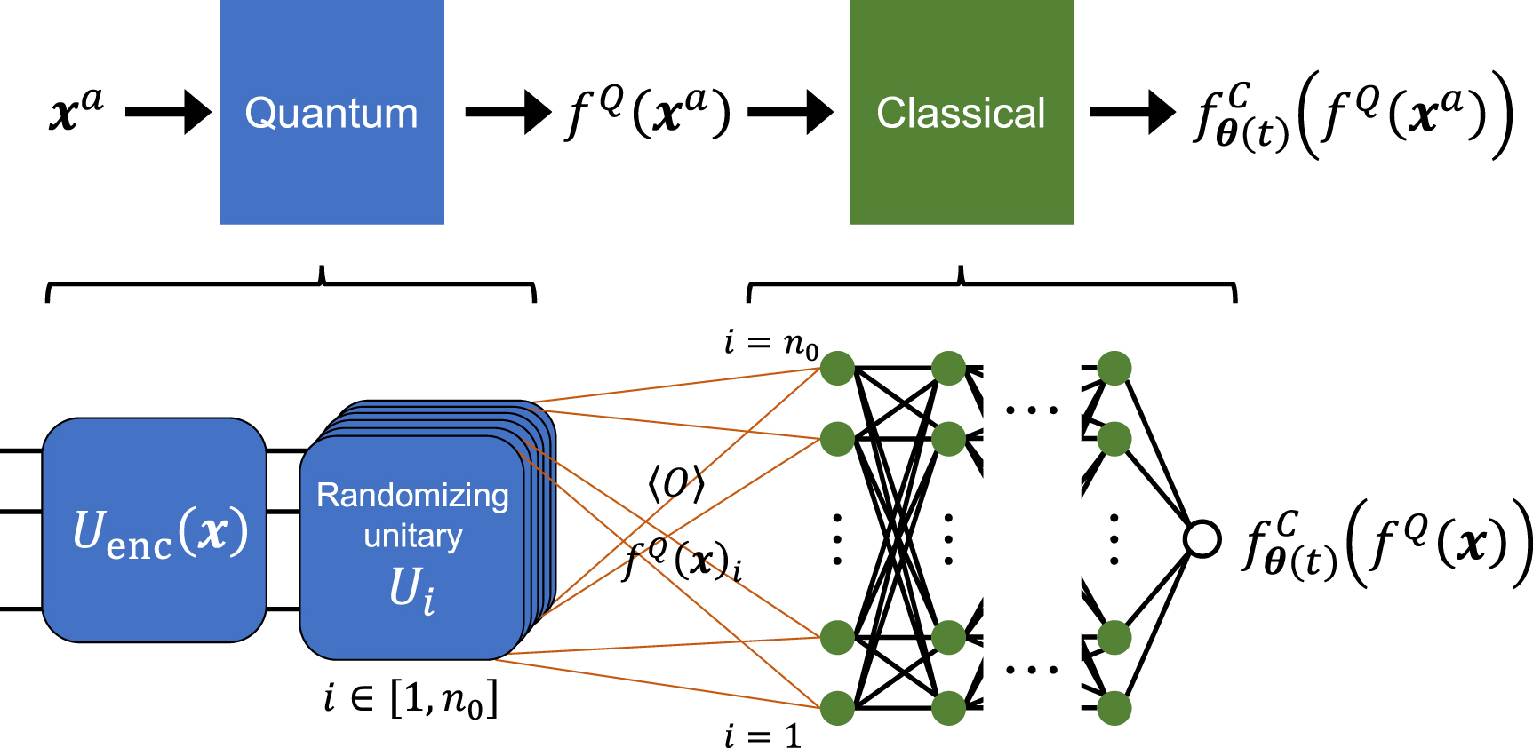
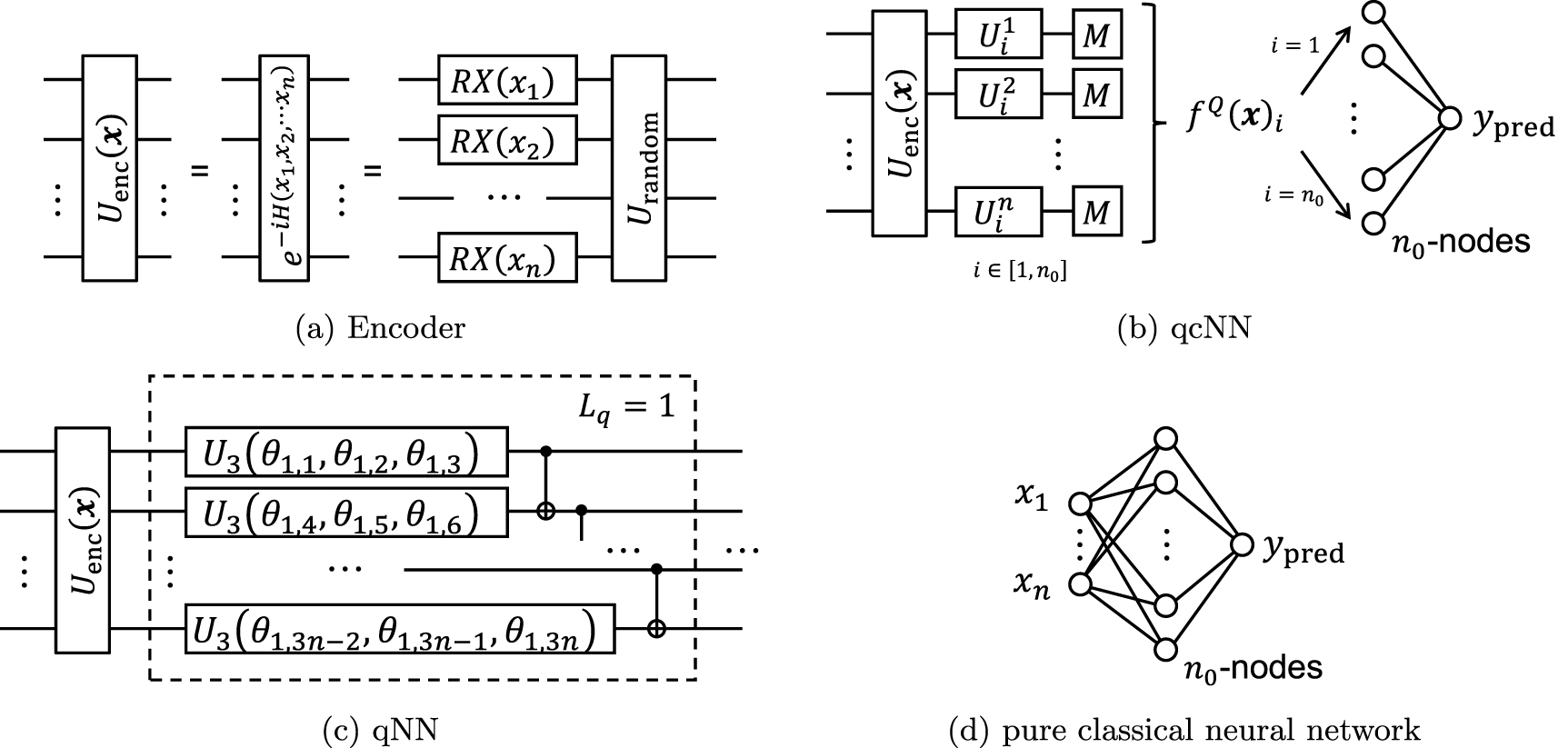