

Abstract
The measurement of transport current density is significant for investigations on improving the properties of REBa2Cu3O7−x (REBCO, where RE refers to rare-earth elements)-coated conductors (CCs). In this work, a protocol for mapping the transport current density of CC by magneto-optical imaging (MOI) is presented. A calibration method is developed based on the non-linear physical governing function for the MOI indicator, in which only two parameters are determined, i.e. the anisotropic magnetic field BA, and cMs, which is the multiplication of the constant c related to the thickness of the MOI indicator and the spontaneous magnetization Ms . The experimental results also showed that they were independent of the optical measure condition but dependent on temperature, making this calibration method comparative among different utilizers. The numerical results clearly manifested that the selected window size of the magnetic field around a long superconducting tape is closely related to the error of the reconstructed current density. A large window size of the magnetic field is needed to precisely reconstruct the transport current density. For actual MOI testing, a practical approach to extend the magnetic field data outside the MOI window was realized by fitting with a power function according to Ampere's law, through which the false current density outside the sample is automatically suppressed to a large extent. On this basis, the mapping of the transport current density in the CC sample was achieved. It is believed that this work will improve MOI for a more precise measurement of the transport current density for long superconducting strips.
Export citation and abstract BibTeX RIS
1. Introduction
REBa2Cu3O7−x (REBCO, where RE refers to rare-earth elements)-coated conductors (CCs) have a multilayered-film structure and serve as one of the key superconducting wires for applications of high-field superconducting magnets [1–3], superconducting transmission cables [4], and superconducting energy storage [5], etc. The critical current of CCs, especially in high magnetic fields, is a significant parameter in their engineering design and applications [6–8]. However, in addition to temperature and applied magnetic field, the critical current is influenced by strains [9–11], grain angles [12], pinning centers [13, 14], defects [15] and damages [16] in superconducting layer. Improving the properties of the superconducting layer so as to achieve a high critical current of CCs requires sufficient investigation of these factors on the CC's current density. Unlike common conductors, the current density distribution for a CC is not uniform but varies along its width [17, 18]. Since there are no direct methods to measure the current density, mapping of the current density distribution is usually reconstructed from the inversion of the magnetic field at the CC surface according to the Biot–Savart law [19–22].
Among the approaches to obtain the magnetic field distribution with high spatial resolution are scanning techniques, such as SQUID [23] or micro Hall-probe array [24], as well as magneto-optical imaging (MOI) based on the Faraday effect [25, 26]. Due to the sub-nanosecond response time [27], MOI is the preferred application for real-time visualization of the magnetic field, including magnetic flux avalanches [28], quench propagation [29], and crack-induced flux penetration [16, 30], etc. For this reason, MOI has mostly been used for quantitativecurrent density analysis of superconducting films, especially for the time-dependent case [31].
Since MOI directly provides the intensity data as a two-dimensional picture, mapping of the current density must start from the inversion of the magnetic field. There have been sufficient studies on the magnetic-induction current density of superconducting films, in which the magnetic field only in the same direction. The magnetic field with different directions of superconducting samples has been observed through light and dark regions or color changes [32–38], but most of these studies only provided only an intensity analysis. Nevertheless, the mapping of the transport current density by MOI has rarely been studied, and only a few related works on the current-carrying micro superconducting bridge have been reported [34, 35, 37, 39]. Investigation of the transport current density distribution of CC by MOI on the macroscopic scale still needs to be well researched, as well as its calibration. It should be noted that there are still several problems to be solved in the reconstruction of the transport current density by MOI: (1) the magnetic field induced by the transport current contains both variables of magnitude and sign. In this case, the common crossed setting of polarizers no longer applies. The adoption of a white light source and uncrossed polarizers in MOI to obtain greenish or yellow pictures [36] was just able to provide qualitative analysis, i.e. on the direction rather than the magnitude of the magnetic field. The other triplet-rotation-angle approach [40] was effective to obtain a high resolution of the magnetic field with magnitude and sign simultaneously, with the aid of an external device to precisely control the rotation plane of polarizing light, which to some extent complicated the MOI system. By practically calibrating a polynomial fit to the relationship between the intensity and magnetic field, we can get rid of the main hindrance of non-uniform illumination [41, 42]. The parameters for calibration strongly depend on the conditions of the light source and camera settings, making it hard to be comparable between different utilizers. (2) The routine MOI experiment starts by recording MOI pictures of samples in the superconducting state below Tc , followed by a calibration process at elevated temperatures above Tc . Though the working temperature range is wide for widely used MOI indicators made from Bi-doped iron garnet, the temperature influence on the properties of the MOI indicator is often neglected during tests. Thus, there is a need to develop a calibration procedure that considers the temperature effect. (3) Physically speaking, the magnetic field generated by a CC with the transport current diffuses through the infinite space; however, information on the detected magnetic field is limited due to the size limit of the MOI indicators, and thus a correlation between the measured space size of the magnetic field and the accuracy of the current density needs to be revealed.
In this work, we address these problems. First, a systematic non-linear calibration process was developed to get rid of non-uniform illumination. In this method, only two parameters of the MOI indicator were determined, both independent of the light and camera setting conditions. In addition, the temperature effects on these two parameters were studied, and an improved procedure for MOI measurement was provided. Second, the relationship between the measured window space size and the accuracy of the current density was investigated, while a practical method for magnetic field extension was proposed for MOI testing in the case where the sample size was comparable to the size of the MOI indicator. Finally, current density reconstructions of the CC were realized with different applied transport currents.
2. Experiment
2.1. Sample parameters
The CC sample used in this experiment is made by Suzhou Advanced Material Research Institute Co., Ltd. Its specifications are listed in table 1.
Table 1. Sample specifications.
| Width | Fabrication technique | Structure | Critical current at 77 K |
|---|---|---|---|
| 2 mm | Ion beam assisted deposition and metal organic chemical vapor deposition | Ag (2  )
YBCO (1 )
YBCO (1  )
Buffer (0.2 μm)
Hastelloy (50 )
Buffer (0.2 μm)
Hastelloy (50  ) )
| 88 A |
2.2. Experimental setup
The experimental setup contains two subsystems: one is a common MOI system, the other a specially-designed cryostat that can apply strain, transport current, and external magnetic field. Details of the cryostat can be found in our previous work [43, 44]. The MOI system consists of an assembled 530 nm LED light source, a pair of polarizers, a beam-splitter prism, and an 8-bit digital camera with macro lens for large-area imaging. The MOI indicator used has a Bi-doped magneto-optical sensor layer of 5 μm, a gadolinium gallium garnet substrate of 500 μm, and a mirror layer of 0.2 µm. The details of the system are shown in figure 1.
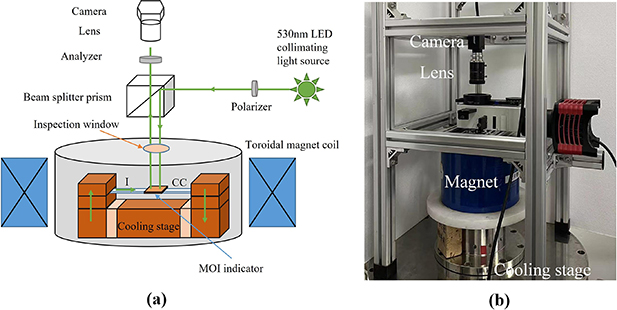
Figure 1. (a) Schematic diagram of experimental arrangement. (b) Photo of experimental device.
Download figure:
Standard image High-resolution image2.3. Calibration
The sensor layer of the MOI indicator has an in-plane spontaneous magnetization Ms without an external applied magnetic field B. If there is an applied B at an angle α to the film plane, the Ms tilts out of the plane with the angle φ, as shown in figure 2.

Figure 2. Schematic diagram of interaction of the applied magnetic field B and spontaneous magnetization Ms . Without the applied field, Ms lies in the film plane, while an external B would rotate the Ms out of plane.
Download figure:
Standard image High-resolution imageThe interaction energy contains magnetocrystalline anisotropy energy and magnetostatic energy [21], as expressed in equation (1):

where  is the anisotropic energy and α is the angle between the applied field and the film plane. At a given α, φ varies with the magnetic field, and the whole process satisfies a minimum energy change, i.e.
Equation (2) requires  , from which we get
where  is the anisotropic magnetic field,
  is the in-plane magnetic field component, and
  is the perpendicular magnetic field component. It should be noted that when there is an applied field strictly perpendicular to the CC, the in-plane magnetic field component will be generated by the in-plane current density flowing in the CC. The Faraday rotation angle αF
, proportional to the z-component of magnetization, is denoted as
is the perpendicular magnetic field component. It should be noted that when there is an applied field strictly perpendicular to the CC, the in-plane magnetic field component will be generated by the in-plane current density flowing in the CC. The Faraday rotation angle αF
, proportional to the z-component of magnetization, is denoted as

where c is a constant that relates to the thickness of the MOI indicator. Using a common MOI system, the light intensity received by the camera is expressed according to Malus' law:

where Imax is the incident light intensity, I0 is the background light intensity, and θ is the initial cross-angle between the polarizer and the analyzer. In an MOI photo, Imax and I0 are usually non-uniform because of the inhomogeneous illumination of the light source and the background intensity of the camera. Here, we develop a new way to get rid of this effect. First, at a set angle θ, the Imax is calculated as Iθ, max without applied magnetic field by
where Iθ,B =0 is the intensity with θ of polarizers and I90°,B=0 is the intensity recorded with the crossed setting of polarizers. Then, by combining equations (2)–(5), the normalized light intensity IN (x,y) as a function of the applied field B is obtained as
Accordingly, the z-component of the magnetic field is calculated as
Equations (7) and (8) are used to calibrate the intensity versus the applied magnetic field and extract the magnetic field from the intensity, respectively.
3. Current density reconstruction from superconducting strip with transport current
MOI measures the z-component of the magnetic field perpendicular to the plane of the MOI indicator, and can be used to reconstruct the two-dimensional current density. Calculation in Fourier space according to the Biot–Savart law is an efficient method. The average current densities Jx and Jy along the thickness of the superconducting film are [22]
where kx and ky are coordinate indices in the Fourier space, h is the interval between the magneto-optical layer and the superconducting layer, and d is the thickness of the superconducting layer. In addition, the expressions for the in-plane components of the magnetic field are
Generally speaking, the magnetic field is distributed over the infinite space with a source current. It should be noted that the acquired magnetic field information for MOI is limited because of the limited size of the MOI indicator. Equations (9) and (10) have proven to work well for the reconstruction of the induced superconducting current density with the limited measured magnetic field by MOI. Nevertheless, for the case of transport current density, i.e. only self-field information is provided, there is a need for careful scrutinization when choosing different window sizes of the measured magnetic field. Here, the analytical results from Brandt and Indenbom [17] were simulated as a numerical experiment. Considering a current I that transports along the y direction in an infinite long superconducting strip as in figure 3(a), the current density along the width (x direction) is
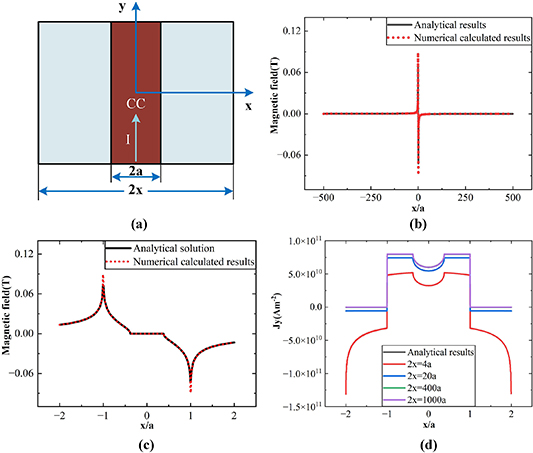
Figure 3. Numerical results of reconstructed current density with magnetic field of different window sizes. (a) Schematic of superconducting strip of Jc
of  A m−2 with a transport current of 120 A. The width of the strip is 2a, and that of the selected magnetic field window is 2x. (b) Comparison of the magnetic field between the numerically reconstructed and analytical results. (c) Enlarged view of (b); note that there are two singularities in the analytical solution at the strip edges that are not plotted. (d) Plots of reconstructed current density with different magnetic field window sizes and analytical one, where only the points of range within ±2a are plotted.
Download figure:
Standard image High-resolution imagewhere  . The z component of the magnetic field is
where  . It should be noted that the current density calculated by equation (13) is continuous, while the magnetic field by equation (14) has two singularities at both strip edges. Thus, a window with a size 500 times as large as the width of the strip was selected here, with which a continuous z-component of the magnetic field was reconstructed with equation (10). This agrees well with the theoretical value except the singularities, as shown in figures 3(b) and (c). Next, magnetic fields with windows of different sizes were selected to reconstruct the current density using the mentioned Fourier calculation, simulating the loss of magnetic-field information during the MOI measurement. The results are plotted in figure 3(d). It was found that the value of the constructed current density did not agree well with the theoretical one unless the window size of the magnetic field was as large as possible. For a small window size, e.g. where the size was just two times the width of the strip, the current density was less than the theoretical one within the strip and had a false value outside the strip.
Here, a practical approach to solve this problem was proposed by supplementing the magnetic field information outside for the case of a small window. Considering that the magnetic field far away from the strip decays scale to x−1 (x denotes the distance from the origin) according to Ampere's law, the decaying behavior can be well approximated using a power function as follows:
where A and B are fitted parameters. Thus, the magnetic field window is expanded to a sufficiently large extent and the current density is reconstructed using the extended magnetic field. For example, as shown in figure 4(a), a magnetic field window size of two times the strip width was first selected and assumed to be measured magnetic field, i.e. within the window, the true magnetic field values were used, while outside the window, the magnetic field values (assumed to be not measured by MOI) were calculated from the data within the outmost magnetic field window of width of 0.4a by the fitted function of equation (15), in such a way, the magnetic field window was then extended from 2 to 500 times of sample width, as in figures 4(b) and (c), followed by the current density reconstruction. Table 2 lists the integrated current results and relative errors with different extended magnetic window sizes. In comparison, the current density with an extended magnetic field window size of 500 times the sample width agrees well with the theoretical one as plotted in figure 4(d), with a relative error of 1.01%.

Figure 4. Current density reconstruction results from extended magnetic field window. (a) Schematic of superconducting strip of Jc
of  A m−2 with a transport current of 120 A. The width of the strip is 2a, the selected magnetic field window size is 4a, the magnetic field from the outmost window of size 0.4a was used to calculate the magnetic field values outside the selected window by the fitted function, and the total extended magnetic field window size is 2x. (b) Extended magnetic field with fitting function, where data within left part of extended window is shown. (c) The whole magnetic field distribution after being extended with an enlarged view inserted. (d) Plots of reconstructed current densities with different extended magnetic field window sizes and analytical one; only the points of range within ±2a are plotted.
Download figure:
Standard image High-resolution imageTable 2. Results of integrated current and their relative errors with different extended magnetic window sizes.
Extended magnetic field window size ( ) ) | 2 | 10 | 200 | 500 |
|---|---|---|---|---|

| 73.2024 | 110.5498 | 118.5426 | 118.7835 |

| 39.00% | 7.88% | 1.21% | 1.01% |
4. Results
4.1. Magnetic field extraction from MOI picture
Considering that the maximum Faraday rotation angle of the polarizing plane in the MOI indicator under an applied magnetic field is in the range of ±10°, the common orthogonal polarizer configuration, i.e. θ equals 90° in figure 5(a), is only able to measure the magnitude of the magnetic field without information of its direction, according to equation (5). Thus, initial angles between 115° and 150° were set so that a monotonic change of intensity versus the applied magnetic field from negative to positive was acquired. As shown in figure 5(b), at the maximum applied magnetic field, the intensity value was set close to the saturation (value of 255 in our 8-bit camera) of the image. It was clear that the largest variation range of intensity existed at 115° and the smallest at 150°; in contrast, the sensitivity at the negative maximum applied magnetic field was smallest at 115°, hence there was a need to find a balance between the intensity contrast and sensitivity during the MOI test.

Figure 5. (a) Schematic of configuration of the polarizer and analyzer. (b) Variation of intensity versus the applied magnetic field with different initial angles between the polarizer and analyzer.
Download figure:
Standard image High-resolution imageTaking an initial angle of 125° as an example, a MOI image of 87.5 mT at room temperature is shown in the inset of figure 6(a), in which 16 sub-areas were chosen to show their dynamic responses under the applied magnetic field.

Figure 6. Intensity variation versus the applied magnetic field in calibration process. (a) The intensity responses of 16 sub-areas of the inserted image taken at room temperature and 87.5 mT. (b) The intensity responses of 16 sub-areas after normalization.
Download figure:
Standard image High-resolution imageDifferent dynamic ranges were caused by the non-uniform illumination. By utilizing the proposed calibration method, all the curves displayed nearly the same behavior, as shown in figure 6(b).
From the calibrated curve that gets rid of non-uniform illumination, the data points are fitted by equation (7) with the least-squared method, resulting in only two parameters, i.e. BA and cMs , which are nearly independent optical measure conditions but only related to the properties of the MOI indicator itself, as plotted in figure 7. However, the results of calibration at different temperatures manifest that the values of BA and cMs depend on different temperatures. When comparing the values of BA and cMs at different temperature, the value of BA is smaller and cMs larger at cryogenic temperatures than they are at room temperature, which as shown in figure 8.

Figure 7. Mean and standard deviation plots of (a) BA and (b) cMs for different θ at room temperature. Results with each angle were measured in four repeated experiments.
Download figure:
Standard image High-resolution image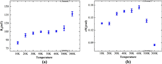
Figure 8. Mean and standard deviation plots of (a) BA and (b) cMs at different temperatures. Results at each temperature were obtained with three different initial angles of polarizers.
Download figure:
Standard image High-resolution imageThe origin MOI pictures of a CC sample with a width of 2 mm and different transport currents under 10 K self-field are displayed in figure 9(a). Using the proposed calibration approach, the extraction of the magnetic field distributions are drawn in figure 9(b).

Figure 9. (a)–(f) are original MOI images of a CC with transport currents of 20 A, 40 A, 60 A, 80 A, 100A, and 120 A at 10 K self-field, respectively. Figures (g)–(l) are magnetic field distributions obtained by the proposed calibration method, in which the influence of non-uniform illumination is removed.
Download figure:
Standard image High-resolution image4.2. Current density reconstruction of CC with transport current
After the extraction of the magnetic field data in the measured window of MOI, the current density is reconstructed through the Fourier calculation as mentioned in section 3. Here, the magnetic field data along the red dotted line in figure 9(a) is focused. If the current density is directly inverted by the measured magnetic field as in figure 10(a), the current density result plotted as in figure 10(b) is very similar to the simulated case of 2x = 4a in figure 3(d). Therefore, the magnetic field outside the MOI indicator was extended with the approach presented in section 3, shown with blue complemented data points as in figure 10(c). Then the current density was obtained as in figure 10(d), eliminating a large part of the false current density outside the sample.
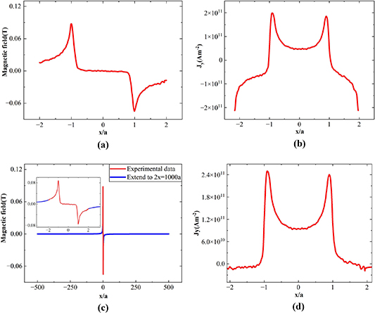
Figure 10. (a) Measured magnetic field profile along the CC width. (b) Distribution of current density reconstructed by the MOI data. (c) Extension of the magnetic field range; red line is the initial measured field data, blue line is the extended data. (d) Distribution of current density obtained by the inversion of the extended magnetic field window.
Download figure:
Standard image High-resolution imageHowever, there are still some false current densities near the edge of the CC. This is thought to be caused by the in-plane field effect, i.e. the influence of the current-induced magnetic field components parallel to the plane of the MOI indicator. The problem here was solved by the approach proposed by Laviano et al [22], in which the z-component of the magnetic field data inside the sample was iteratively corrected as in figure 11(a). The corresponding corrected current density is plotted in figure 11(b).

Figure 11. (a) Magnetic field distribution before and after iterative correction; (b) reconstructed current density before and after iterative correction.
Download figure:
Standard image High-resolution image5. Discussion
In the calibration process, equation (8) is used to calcalate the magnetic field on the basis of eliminating the non-uniform effect of optical illumination. In comparison with other calibration methods, such as the polynomial-fitting , the proposed approach can realize the conversion from intensity to magnetic field only by providing parameters BA and cMs about the physical properties of MOI indicator. The merits of the MOI indicator parameters remain unchanged with changes in optical measure conditions, making the results to be comparable between different users.
In addition, for common MOI tests on superconducting samples, MOI pictures are usually taken at temperatures below Tc , and calibration is done at temperatures above Tc , hence temperature-induced changes on the MOI indicator as well as the induced corresponding errors were always neglected. In section 2.3, we develop a calibration method, which just needs to be conducted without a superconducting sample at cryogenic temperature, then the calibrated parameters of BA and cMs can directly be reused for the superconducting case at the corresponding temperature, minimizing the temperature effect on the measured results.
The size of the MOI indicator determines the window size of the measured magnetic field data, in the case of just magnetic field-induced current, and the influence of the measuring window size on current density construction was seldom considered and often neglected. It is physically explained that the magnetic field outside the superconducting sample decays quickly, as shown in figure 12(a), because the directions of current within the two halves of the strip are opposite to each other, resulting in the magnetic fields outside the strip being compensated by the opposite currents. The further away from the strip, the more complete the compensation, thus the reconstruction of the induced current density is less sensitive to the measuring window size, as depicted in figure 12(c). For the case of transport current (where the currents in the strip are the same), the measuring window size effect needs to be considered so that proper construction of the transport current density is attained. Based on the investigations above, a flow chart for mapping the transport current density of CCs is drawn in figure 13.
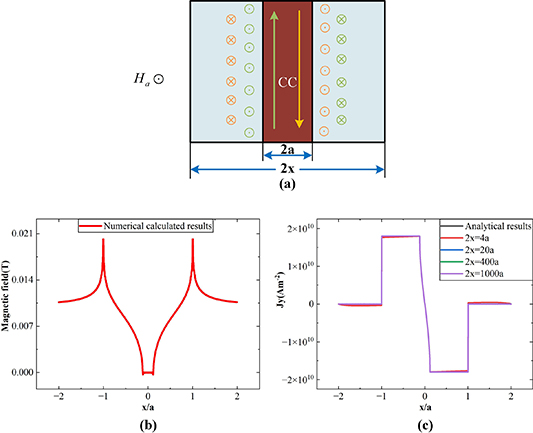
Figure 12. Reconstruction of current densities in the case of induced current. (a) Schematic of a long superconducting strip with induced current under an applied magnetic field. (b) The numerical simulated magnetic field distribution along the CC width. (d) Reconstructed current densities with different magnetic field window size.
Download figure:
Standard image High-resolution image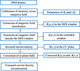
Figure 13. Flow chart for mapping transport current density of REBCO CCs.
Download figure:
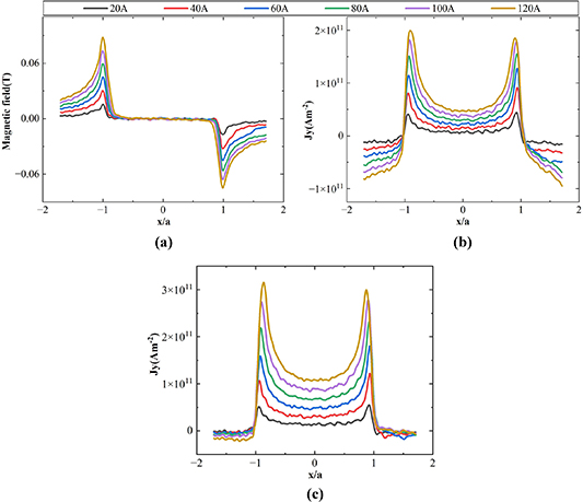
Standard image High-resolution imageIn the case of a CC sample with increased applied current, the magnetic field along the width of the CC was plotted as in figure 14(a), showing the elevated magnitude of the magnetic field near the edge of the sample. Using a common method to perform current density inversion with a limited magnetic field window, the false current density outside the sample becomes remarkable when increasing the applied current, as in figure 14(b). By using the protocol presented, a reasonable current density distribution was obtained, as shown in figure 14(c).
Figure 14. Results of reconstructed current densities with different transport currents. (a) Measured magnetic field distribution by MOI. Figures (b) and (c) are current densities reconstructed by the directly converting method and by the presented protocol, respectively.
Download figure:
Standard image High-resolution image
6. Conclusion
In this paper, we present a protocol for mapping the current density of CCs with a transport current. A calibration method was developed based on the non-linear physical governing function for the MOI indicator, in which only two parameters, BA and cMs , are obtained. Both parameters are independent of the measuring conditions, but dependent on the temperature. The MOI measurement with the superconducting sample should use parameter values of BA and cMs as close as possible to the corresponding temperature.
Current density inversion for the case of transport current should be implemented with a large window size of the magnetic field. Choosing the long strip as a simple geometry, it was found that little error in inverted current density was obtained with a magnetic field window size 500 times large as the width of the strip. For practical MOI measurements, the magnetic field outside the MOI window was extended by fitting with a power function according to Ampere's law, through which the false current density is automatically suppressed to a large extent. It is believed that this work will advance MOI for a more precise mapping of the transport current density.
Acknowledgments
All the authors thank Suzhou Advanced Material Research Institute Co., Ltd for the free samples.
Data availability statement
Raw experimental data shall be provided for proper requirement.
All data that support the findings of this study are included within the article (and any supplementary files).
Conflict of interest
The authors declare no conflicts of interest.
Funding
This work was supported by the Fund of Natural Science Foundation of China (Nos. 12272155, U2241267, and 12232005) and Gansu Association for Science and Technology of China (No. GXH202220530-18).