
Efficient and choreographed quality-of- service management in dense 6G verticals with high-speed mobility requirements
Abstract
Future 6G networks are envisioned to support very heterogeneous and extreme applications (known as verticals). Some examples are further-enhanced mobile broadband communications, where bitrates could go above one terabit per second, or extremely reliable and low-latency communications, whose end-to-end delay must be below one hundred microseconds. To achieve that ultra-high Quality-of-Service, 6G networks are commonly provided with redundant resources and intelligent management mechanisms to ensure that all devices get the expected performance. But this approach is not feasible or scalable for all verticals. Specifically, in 6G scenarios, mobile devices are expected to have speeds greater than 500 kilometers per hour, and device density will exceed ten million devices per square kilometer. In those verticals, resources cannot be redundant as, because of such a huge number of devices, Quality-of-Service requirements are pushing the effective performance of technologies at physical level. And, on the other hand, high-speed mobility prevents intelligent mechanisms to be useful, as devices move around and evolve faster than the usual convergence time of those intelligent solutions. New technologies are needed to fill this unexplored gap. Therefore, in this paper we propose a choreographed Quality-of-Service management solution, where 6G base stations predict the evolution of verticals at real-time, and run a lightweight distributed optimization algorithm in advance, so they can manage the resource consumption and ensure all devices get the required Quality-of-Service. Prediction mechanism includes mobility models (Markov, Bayesian, etc.) and models for time-variant communication channels. Besides, a traffic prediction solution is also considered to explore the achieved Quality-of-Service in advance. The optimization algorithm calculates an efficient resource distribution according to the predicted future vertical situation, so devices achieve the expected Quality-of-Service according to the proposed traffic models. An experimental validation based on simulation tools is also provided. Results show that the proposed approach reduces up to 12% of the network resource consumption for a given Quality-of-Service.
1.Introduction
Future 6G networks [1] are characterized by a strengthened Quality-of-Service (QoS) [2], whose objective is to support a heterogeneous catalogue of new applications and scenarios [3]. However, it is very complicated to satisfy the needs of all those applications through a unified and homogeneous network architecture [32]. In this context, 6G networks define “verticals” [4]. 6G verticals are commercial niches where providers cater to a particular target group, allocating and isolating the required network resources, implementing application-specific algorithms and configurations and providing exactly the needed Quality-of-Service [5].
Although some 6G verticals are well-known standard applications, the main difference between 6G and other previous mobile technologies [6] is its extension to very extreme scenario. Dense 6G verticals, those including up to (or even more than) ten million devices per square kilometer, with high-speed mobility requirements (with speeds up to five hundred kilometers per hour), although they are unexplored, are quite common. For example, mass transportation systems (such as high-speed trains or air traffic) match this description and are part of these verticals.
Typically, solutions to achieve the expected QoS in 6G networks are based on the provision of redundant network resources and intelligence management mechanisms [11]. But these solutions cannot be applied to dense verticals, as they are not scalable and, besides, cannot converge fast enough to a stable solution. Actually, as device density increases, redundant resources must be significantly increased too, but they do not have a direct impact on the provided QoS. Furthermore, in some extremely dense verticals (i.e. those including more than ten million devices per square kilometer), it is not clear if enough redundant resources can be physically provided. On the other hand, intelligent mechanisms have a non-negligible convergence time [15]. But, for example, in long-distance and high-mobility communications (LDHMC) [16] devices are expected to move and evolve at speeds greater than five hundred kilometer per hour. So, a stable network configuration can never be achieved as device distribution evolves more quickly than QoS management intelligent schemes can converge.
Then, innovative network and QoS management solutions, addressing the pending open challenges and adapted to those dense 6G verticals and LDHM requirements are needed.
Therefore, the objective of this paper is to develop a new proactive choreographed Quality-of-Service management solution for dense 6G verticals with high-speed mobility requirements. The proposed solution is based on a lightweight optimization algorithm that can be operated at real time, based on information generated in advance (predicted) by base stations in a distributed and collaborative way. The optimization objective will be defined by a set of QoS indicators. The future value of these indicators will be estimated using a probabilistic network traffic model. The optimization algorithm is fed with the estimate future state of devices within the vertical. To obtain that estimation, the current mobility state of devices is calculated using models for time-variant communication channels and taking advantage of ultra-directive antennas employed in 6G base stations. Additionally, the future mobility state of devices is obtained using different lightweight models operating at real time (Markov, Bayesian and conventional probabilistic models), and a majority voting process to ensure the best estimation is considered. The optimization algorithm calculates an efficient resource distribution based on the predicted future vertical’s situation, so devices achieve the expected Quality-of-Service according to the proposed traffic models. Redundant resources are needed, and mobile network is fully prevented.
The rest of the paper is organized as follows. Section 2 presents the state of the art on 6G mobility and Quality-of-Service management solutions. Section 3 presents the proposed solution, including the optimization algorithm and all required models. Section 4 describes the experimental evaluation; Section 5 discusses the obtained results; and Section 6 concludes the paper.
2.State of the art
In this section we analyze the state of the art on Quality-of-Service and mobility management solutions for 6G networks. Next subsections study those two topics.
2.1Optimum QoS management solutions in dense 6G verticals
First, technologies at physical level have been reported. In this approach, complex parametric models for radio channel capacity (throughout) [20] or received radio power [21] are proposed. But some of these models do not have closed-form expressions, so the only feasible option to evaluate those models is through exhaustive simulations, which required very large processing periods. That is totally incompatible with high-speed mobility requirements. Some authors have proposed employing neural networks, including adversarial and/or generative networks [9], to deal with these not closed-form expressions [22], but in many cases the resulting numerical problems are nonconvex [23] and then the convergence time for these artificial intelligence approaches is too much higher than usual. So high-speed mobility requirements are not met neither.
Table 1
State of the art in QoS and mobility management
| References | Management approach | Supporting technology | Comments |
|---|---|---|---|
| [20][21][22] | QoS | Optimization algorithms | Large convergent and solving periods |
| [28][29][30][31] | QoS | Artificial intelligence | Precision and convergence are not guaranteed |
| [17][35][36][55] | QoS | Traffic engineering | Only able to optimize bitrate |
| [40][41][44] | Mobility | Lightweight handovers | 6G dense verticals are not supported |
| [42][43] | Mobility | New network architectures | 6G dense verticals are not supported |
| [45] | Mobility | Clustering | Only able to optimize bitrate |
| [47] | Mobility | Goniometry | Not all 6G dense verticals are supported |
| [48][49] | Mobility | No solution. Pending challenges | Not all 6G dense verticals are supported |
| [50][51] | Mobility | Bayesian networks | Large calculation delays in dense 6G verticals |
| [52][57] | Mobility | Markov chains | Low precision |
Intelligent solutions are also used at link or network level [24]. Supervised learning is usually employed at the lowest level, in controllers for channel estimation [28] or interference management [29]. Unsupervised learning, on the other hand, typically operates at network level within node clustering algorithms [30] and multipath tracking protocols [31]. However, in these intelligent schemes, the Universal Approximation Theory only guarantees the approximation errors tend to zero as the calculation steps (and the number of neurons, is applicable) go to infinite, just if the optimal QoS distribution is a deterministic and continuous function [20]. But when high-speed mobility requirements are considered, QoS is not deterministic, but probabilistic. Intelligent solutions, then, tend to be unprecise and non-convergent. Our proposal addresses this open challenge.
Other solutions based on graph theory [19] and traditional traffic engineering mechanisms have also been studied [33]. Mainly, queue management algorithms including Markov models [17], queue theory [55], traffic classification [35], self-adaptive approaches [14] and/or congestion control [36] have been proposed. In general, however, these ad hoc solutions are specifically designed for a particular device density and speed. And, more importantly, they are only able to optimize one QoS indicator (usually throughput or communication delay). But 6G verticals show multidimensional dynamic QoS requirements and restrictions that need a more flexible and holistic approach to QoS management. This work fills this gap.
Table 1 summarizes the main approaches for QoS management in 6G networks reported in the state of the art.
2.2Mobility management solutions in 6G
Mobility management is one of the key challenges in mobile communications systems. Traditional approaches to this area focus on mitigating the impact of mobility on radio signals or network protocols [37]. But in dense 6G verticals, the impact of the large number of mobile devices moving around may be unpredictable and may even cause the base stations to become congested and collapse [38]. Then, mitigation is not enough, and new proactive management techniques are being studied and proposed.
Two basic approaches to mobility management in 6G networks have been reported [39]: handover management and location management.
Handover management techniques are focused on reducing the required time to complete a handover. It is the most time-consuming control process, as it requires around fifty second to succeed, while (for example) high-speed trains only need eleven seconds to go through the coverage area of a standard base station [40]. Smart signalization solutions have been proposed at the physical level, where implicit (doppler) information in radio signals is used to reduce the exchange of information between user devices and base stations have been proposed [40]. Other mechanisms at link level propose new protocols for 6G handovers with a reduced number of messages to be exchanged [41]. Some of these schemes even enabling low-latency communications [44]. Other solutions consisting of innovative networks architectures have also been reported. Schemes can be found where specific severs and databases manage mobile devices [42] and solutions where handovers are device-to-device with reduced network intervention [43].
But those previous works present some disadvantages. First, they focus on scenarios with a reduced or standard device density. But in dense 6G verticals, the handover processing delay is negligible compared to the context update delay in base stations (which is not optimized), so no real significant improvement can be achieved through these methods.
Besides, those works are only able to improve one QoS (delay), but not all verticals present hard restriction with latency, and other indicators (bitrate, reliability, etc.) may be relevant instead. Finally, most of these proposals, networks cannot follow commercial or scientific standards, which is undesired.
Some works specifically focused on dense 6G verticals can be found, but they are sparse and totally focused on increasing network throughput [45]. More general solutions are required, and, moreover, some authors have warned that any realistic solution for 6G dense verticals needs to consider QoS and resource management together [46].
On the other hand, location management technologies aim to capture the devices’ location, so the network can be optimally configured to that geographical distribution. At the physical level, solutions have been reported for base stations that work with millimetric waves to adjust the radiated power to the number of devices in their coverage area [47]. But the most common work in this area is focused on the non-terrestrial segment [49]. Schemes are being investigated to ensure that 6G networks can locate and follow moving elements such as planes or satellites [48] and guarantee they are correctly served. Although reported proposals are preliminary (focused on challenges, possible solutions, etc.) and only prospective [49]. Anyway, these mechanisms are very application-specific and cannot be implemented in all 6G dense verticals.
Finally, some authors are exploring techniques to predict the future location of mobile devices, so 6G networks can prepare in advance to the future system situation. Typical approaches to that problem are based on Bayesian networks [50], which can be combined with other technologies such as neural networks [51] to improve the precision. These techniques have proven to be successful, but too slow for high-speed mobility scenarios. On the contrary, faster mechanisms based (for example) on Markov chains [52, 57] achieve much lower precision.
Table 1 summarizes the main solution for mobility management in 6G networks.
In this paper, we fill this gap, with a holistic approach to mobility, QoS, and resource management. All these three dimensions are considered together. Besides, to harmonize models with a good precision but lightweight enough to operate at real-time in scenarios with high-speed mobility restrictions, a choreographed and collaborative calculation process is proposed.
3.A choreographed QoS management solution
In this Section, the proposed choreographed QoS management solution is described. Figure 1 shows a block and flow diagram for the proposed solution.
Figure 1.
QoS management solution (block and flow diagram).
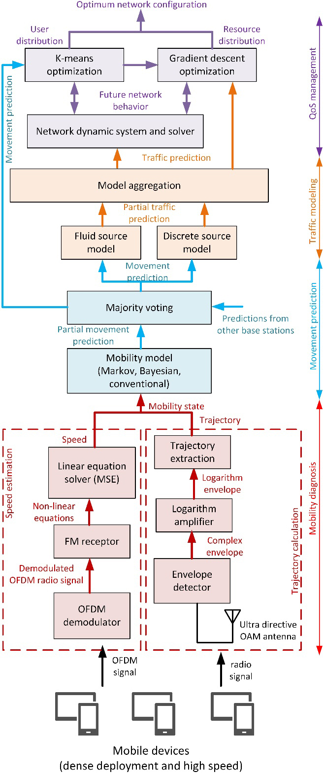
In general words, with this new technology, 6G networks can calculate the optimum device distribution among existing base stations. Therefore, network resources are allocated in such a way that all devices operate with the expected QoS, even under extreme density and extreme mobility requirements. The proposed solution (see Introduction) must be very scalable (to allow very dense verticals) and require a reduced computational effort (to allow extreme mobile devices). This new mechanism captures the current device trajectory and speed using analog and numerical techniques (which require a reduced computational cost) and uses this information to predict its future position and data exchange. With these predictions, the future optimum network configuration can be deduced in advance. As complex predictive methods are computationally heavy, predictions are based on probability numerical models, which are updated and aggregated in a decentralized and unstructured but coherent (choreographed) way.
The proposed choreographed solution is the result of exhaustive numerical investigations, where different parameters and variants were analyzed. An iterative and heuristic procedure was followed. To the best of our knowledge, this is the first time that mobility prediction models and traffic engineering models are combined and customized to define a QoS optimization problem.
The application scenario consists of a dense set of mobile devices with high-speed mobility requirements. To serve all these devices, the 6G network uses a specific vertical that includes a limited number of interconnected base stations. Each one of these base stations is provided with a mobility diagnosis module to capture the current mobility state of devices. The mobility state of any device is described using two different parameters: speed and trajectory. Each of these parameters is captured in the mobility diagnosis module using a specific algorithm. Both algorithms are executed in parallel and at real-time.
The speed estimation procedure takes advantage of the Doppler effect that appears in radio signals when devices move at high speed. This estimation process starts with a partial OFDM (Orthogonal frequency division multiplexing) demodulation. With these partially demodulated radio signals, we can create a new signal containing the output of a randomly time-variant linear radio channel within its phase. Through FM (Frequency Modulation) receptors, this signal is transformed into a set of linear equations which is solved using the Mean Squared Error (MSE) minimization technique. The result of this process is the estimated speed of the devices.
On the other hand, the trajectory calculation algorithm takes advantage of ultra-directive array antennas in 6G base stations. 6G base station will be provided with Orbital Angular Momentum (OAM) antennas, which show very narrow orthogonal beams (or modes). Differences in how radio signals are received through each one of these beams can be used to calculate the devices’ trajectory just employing an envelope detector, a logarithmic amplifier and a trajectory extraction algorithm based on simple mathematical operations and a linear equation numerical solver.
Using the captured devices’ mobility state, each base station can perform a prediction about the future geographical distribution of devices across the vertical. In order to guarantee that the proposed solution is lightweight, efficient, and can operate at real time, but at the same time is very precise, each base station employs a different prediction technique which are later combined through a majority voting scheme. The movement prediction module can implement three different techniques (depending on the base station): Markov models, Bayesian models or conventional probabilistic models. These models are lightweight and the final precision is greatly improved by combining all resulting predictions. In all these models, the geographical area covered by the 6G vertical is divided into a square reticulum, and the future distribution of devices across this reticulum is predicted.
Different base stations may get different movement predictions. First, because they are using different models and later because they could have obtained different mobility states for devices. The final prediction is obtained in a choreographed manner through a majority voting process. This technique chooses as final movement prediction the one which maximizes the joint probability of all partial predictions and current mobility state. In order to ensure good behavior or the majority voting algorithm, in our solution, the network managers should guarantee that all three prediction techniques are represented in the vertical in an equivalent proportion.
Finally, the movement prediction must be transformed into specific network traffic parameters. To do that, in the traffic modeling module, Markov models are employed to calculate the expected traffic associated to the predicted movement. As devices may behave in different ways, two different traffic Markov traffic models are combined: discrete source models and fluid source models. Models are aggregated to calculate the finally raw and global predicted future traffic load within the 6G vertical.
Then, the QoS management module calculates how to distribute all devices within the dense vertical among the different available base stations, and how many resources get each device, so all devices get the required QoS, and base stations are not congested. To do that, this module employs a bidimensional optimization solution based on the K-means algorithm and the gradient descent optimization algorithm. These algorithms need a target function to be optimized. The K-means algorithm is in charge of optimizing the distribution of devices among the different base stations and employs as target function a Euclidean distance. The gradient descent optimization algorithm calculates the resources to be assigned to each device, maximizing as a target function the mean squared deviation of the received QoS compared to the expected QoS.
Both optimization algorithms are connected through a differential dynamic system describing the network behavior, including the network congestion and the provided QoS for each one of the potential optimum distributions. For each possible solution, this dynamic system may be solved using numerical methods, to get the expected network behavior.
Next subsections describe with details each one of the introduced phases, algorithms, and modules.
3.1Mobility diagnosis
A dense 6G vertical with high-speed mobility requirements is composed of a set
(1)
(2)
Every device
(3)
Radio channels are usually linear and time-invariant, but mobile devices with high speed induce a Doppler frequency shift into the radio spectrum which cannot be described with a time-invariant impulse response. Then, under those conditions, radio channels are still linear but randomly time-variant. Then, the OFDM output signal of a time-variant radio channel
(4)
(5)
(6)
In our scenario, time-variant radio channels cause two basic effects: a propagation delay (because of the distance between every device and radio stations) and a Doppler frequency shift because of the fast movement. But this bidimensional kernel function belongs to the time domain, whereas Doppler effects are much easier to describe in the frequency domain. Then we describe the kernel system function as the inverse Fourier transform of a Delay-Doppler-Spread (DDS) function
(7)
(8)
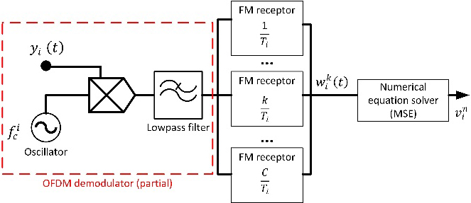
Figure 2.
Speed estimation: Block diagram.
As devices move at very high speed, radio signals show multipath propagation (direct path, scattered paths and reflected paths, mainly). In our model for the DDS function, we assume
(9)
(10)
The first parameter to describe the current mobility state of devices is speed
(11)
(12)
In the base station, OFDM signals are processed with a hybrid receptor mixing a partial OFDM demodulator and an FM receptor (see Fig. 2).
First, signal
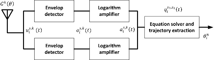
Figure 3.
Trajectory calculation: Block diagram.
These receptors may be implemented using several different techniques (filters and envelope detectors, voltage-controlled oscillators, etc.), but (mathematically) all of them apply a differential operation over the
(13)
(14)
(15)
(16)
Now, considering the relation between the Doppler frequency shift and the devices’ speed, we can obtain a linear Eq. (3.1) with only one unknown variable (the current devices’ speed). But we obtain a similar equation for each OFDM subcarrier, so we get a system of
(17)
(18)
(19)
On the other hand, the same OFDM radio signal
(20)
The OAM antenna is, then, connected to a bank of envelope detectors and logarithm amplifiers, so the devices’ trajectory can be calculated (see Fig. 3). If we exclude devices moving vertically (a very unusual situation), this trajectory (the movement direction) is represented by the reception azimuth angle
(21)
Then, for each sub-beam, an envelope detector is employed to get a new signal
(22)
Then, signals
(23)
Finally, these signals
(24)
(25)
(26)
3.2Movement prediction
After the mobility diagnosis phase, every base station is provided with a set of two parameters
(27)
Figure 4.
Movement prediction: Rectangular grid.
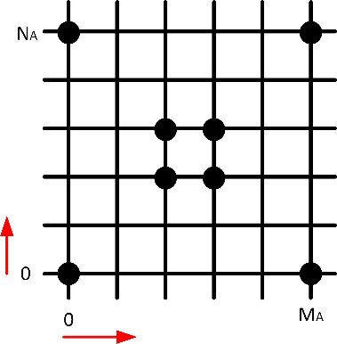
In the movement prediction phase, each base station must calculate a prediction for the future position of every device for which it obtained the mobility state. To do that, each base station may implement a different algorithm. Three possible algorithms are considered in our proposal: conventional probabilistic models, Markov models and Bayesian models.
In the conventional probabilistic model, the future device’s position
(28)
Within this locus, the most probable future locations
(29)
Other future locations may be possible as well, as the extracted current mobility state presents a certain (relative) estimation error
(30)
Parameter
(31)
(32)
Finally, in order to ensure the aggregated probability of all possible future locations
(33)
Conventional probabilistic models require a low computational power to be computed and meet the requirements of ultra-dense verticals; however, are not able to learn. Therefore, the prediction error remains constant as time passes. On the other hand, the Bayesian model can integrate an a posteriori correction process, so the model is constantly improved.
The probability computed using the conventional probabilistic model may be understood as a prior probability
(34)
But a much more precise estimation is provided by the posterior probability
(35)
(36)
Additionally, the conditional probability
(37)
BeingFinally, the Markov model for movement prediction is based on previous observations (locations and mobility states). While conventional probabilistic models and Bayesian models are very fast to compute (faster than ultra-mobile devices), they may be not enough precise when devices show unusual behavior.
In a latent (hidden) Markov model, we assume that the
The probability of the
(38)
(39)
In a Markov model, each location
(40)
However, behaviors
(41)
(42)
As behaviors are not observable, all these parameters must be estimated from observable variables. In our model, these observable variables are the mobility state
First, we are considering all behaviors have the same probability, so
(43)
(44)
(45)
As probabilities
(46)
Regarding parameter
(47)
Algorithm 1 shows the final calculation process of the Markov mobility model.
| Algorithm 1: Markov movement prediction |
|---|
| Input Mobility state |
| Previous paths |
| Previous locations |
| Output Probability of all future locations |
| for all locations |
| Initialize |
| while |
| Calculate |
| Calculate |
| Calculate |
| Calculate |
| Calculate likelihood |
| Calculate |
| end while |
| end for |
Physical noise in the original radio signals
As different base stations are using different prediction models and may get different results, the final future vertical’s situation is obtained through a choreographed majority voting algorithm. With the implementation of three different models, we ensure our proposal can operate under very different requirements: ultramobility, ultradensity, etc. But hereinafter all base stations must agree in a common movement prediction in a choreographed manner.
Being
(48)
(49)
(50)
3.3Traffic modeling
In order to trigger a QoS management algorithm, it is necessary to transform the predicted future location of devices into a prediction of the future network load or traffic. To do that, different models may be employed. Depending on the behavior of each device, it could be considered a fluid source or a discrete source.
In the proposed traffic model, devices may be in two different states: ON state and OFF state. In the ON state, devices transmit and receive data packets at a maximum (peak) bitrate
Regardless of the traffic model, the effective sustainable bitrate
(51)
On the other hand, the effective bitrate
(52)
(53)
Finally, in order to estimate the probability of ON state
(54)
Now, the discrete source model is characterized by a transition matrix
And using the Markov theory,
(55)
(56)
(57)
On the other hand, the transition matrix for a fluid source
(58)
(59)
(60)
As devices can change their mobility state and/or their traffic profile dynamically, it is important to ensure all previous observations, records, and trajectories (including parameters
(61)
This is the easiest way to deprecate information, as models do not have to be modified. But it requires having a large enough number of data
(62)
3.4QoS management
With all previously collected information, two final decisions have to be made in order to optimize the provided QoS within the vertical: how devices are organized to be served by the different base stations and how many resources (bitrate and reliability) are assigned to every device.
The QoS received by the
(63)
In this model, all variables depend on time, but this dependency is not explicitly represented for simplicity. Besides the total capacity provided by each base station is
(64)
The aggregated bitrate
(65)
In those conditions, we must find the maximum (peak) bitrate
(66)
Now, it is possible to define the optimization problem to be solved Eq. (65). This problem may be solved through different standard algorithms. In our proposal we are using a gradient descent optimization algorithm. Specifically, the Adagrad algorithm [25]. Although other could be used as well.
(67)
At this point, it is only needed to calculate which devices
Given a (squared) geographical area
devices to be in that area at the future time instant
(68)
In order to calculate the optimum values for
Thus, the K-means algorithm obtains a solution
(69)
(70)
As the movement prediction was agreed among all base stations in a choreographed manner, all base stations could solve the optimization problem in their own and get the same solution. That highly reduces the negotiation processes and their associated delays.
Finally, to choose which specific devices
4.Evaluation and discussion
In order to validate the proposed technology as a valid solution for QoS management in dense 6G vertical with high-mobility requirements, an experimental validation was conducted. The experiments were supported by simulation scenarios, as real 6G hardware equipment is not still available. Simulation tools have been shown to be a valid experimental strategy before under similar conditions [8].
To perform the experiments, the simulation scenario was implemented and executed using MATLAB 2017a software. Although MATLAB offers different programming interfaces, we are using its native scripting language to implement all the algorithms and the scenario. We chose this platform because it enables parallel computing in multicore machines (cluster), together with a large catalog of numerical libraries and instruments.
All simulations were performed using a Linux architecture (Ubuntu 20.04 LTS) with the following hardware characteristics: Dell R540 Rack 2U, 96 GB RAM, two processors Intel Xeon Silver 4114 2.2G, HD 2TB SATA 7,2K rpm.
The proposed solution was analyzed from two different points of view. A first set of experiments was designed to analyze and test the mathematical properties of the described technology, such as the optimization error or the precision of the model. The second group of experiments was designed to evaluate the performance of the proposed technology in a real scenario and to determine how it meets the initial requirements of 6G networks. Those experiments include a study of the processing delay or scalability.
The proposed simulation scenario represents a suburban area with a low population and construction density (i.e., a density of forty people per square kilometer) and an extension of twenty square kilometers (this can be considered a rural environment in some regions). The location of the constructions will be organized according to an orthogonal grid.
We are considering the atmosphere to have standard conditions, so radio channels are affected by common transmission losses plus those caused by vapor and oxygen. MATLAB function gaspl was employed to simulate the atmosphere and its power absorption.
In this scenario, nine 6G base stations are included. Base stations are uniformly distributed across the entire area under study. The working frequency for this 6G vertical is 244–246 GHz (as envisioned for this new technology) [18] and the transmission power 6G dBm. All of those values are usual in envisioned 6G mobile systems. OFDM radio spectrum, waveforms and propagation models were provided by the MATLAB 5G toolbox. Through the nrDLCarrierConfig object we customized the waveform to be compatible with future 6G networks. The appropriate Doppler effect was generated by parametrizing the waveform with the device speed. Besides, functions such as nrSymbolDemodulate, or nrPolarDecode allowed us to demodulate and decode signals. FM receptors were implemented using the fmdemod function. The final speed and trajectory estimations supported by a MSE minimization problem was implemented through immse (MSE calculation) and fmincon (minimization algorithm) functions.
All communication channels in the scenario followed a probabilistic standard model, provided by MATLAB libraries, and the Communications Toolbox, such as the awgn function. Interferences, transmission errors and dropped packets were randomly introduced according to a Gaussian distribution whose parameters represent the QoS provided to every mobile device at each moment (see Section 3.4).
Various mobility models (Bayesian, Markov, and standard) were uniformly represented and implemented in three different base stations. Algorithms were implemented using common MATLAB scripts, executed in the MATLAB graphical environment. Differential equations in the traffic models were solved using the ode 45 solver, from the most classic MATLAB libraries. Initial values were randomly generated. On the other hand, the Adagrad algorithm for the QoS management model was supported by the “Gradient Descent Optimization” library (downloaded from the official online repositories). The geographical area under study is represented by a square grid (see Section 3.2 and Fig. 4) with a variable number of divisions (independent variable for our experiments). Additionally, the measurement period
On the other hand, the device density in the area is also variable, but limited to the expected densities in 6G verticals (10 million devices per square kilometer at maximum). Additionally, the speed of every device is also randomly established. The interval will range from zero to a maximum speed that will vary as an independent variable. In any case, this maximum speed will never be above five hundred kilometers per hour (the speed of bullet train, the fastest terrestrial vehicle). Other aerial or spatial vehicles might achieve higher speeds, but our model is bidimensional (see Section 3.2) and only suitable for terrestrial applications.
Regarding the trajectories of the devices, they were defined as closed curves within the study area. Four basic kinds of trajectories were considered: ovals, spirals, cycloids, and rhodoneas. Every device is randomly provided with a different trajectory.
Finally, the QoS required for each device is also randomly established. Bitrate demanded by each device varied between 100 Mbps and 10 Gpbs. The reliability must be, at least, equal to 99.999%. All these values are consistent with the performance described for future 6G verticals [7].
Table 2 shows a summary of all the variables and their value, according to previous descriptions.
Table 2
Configuration parameters
| Parameter | Value | Parameter | Value |
|---|---|---|---|
|
| Variable |
| 6 |
|
| 9 |
| 24 dBi |
|
| 3300 |
| Variable |
|
| 4.2 |
| 20 Km |
|
| 8 |
| Variable |
|
| 28 GHz |
| Variable |
All simulations represented an operation time of seventy-two (72) hours. Each simulation was repeated twelve times, and final results were obtained as the average of all partial results. To ensure the verisimilitude of the results, any outlier simulation was discarded and repeated. Until twelve valid simulations were accumulated. Outliers were identified using “geometric criteria”. Specifically, the Mahalanobis distance [54] was used. Mahalanobis distances were later transformed into probabilities. If the probability of the Mahalanobis distance to be greater than the Chi-squared distribution with equal degrees of freedom was greater than 0.95, simulation was considered an outlier and was discarded.
4.1Numerical analysis: Methodology
In order to analyze the behavior of the proposed technology from a numerical point of view, we need to study the (global) error associated with the described algorithms.
To do that, we designed three different experiments. In the first experiment, the relative global optimization error is measured, to discuss the mathematical convergence of the proposed choreographed technology.
In the second experiment, the error associated with the mobility diagnosis phase is captured and analyzed. Finally, in the third experiment, the error associated with the choreographed movement prediction phase is studied.
Each one of these three experiments is, besides, composed of two sub-experiments. In the first sub-experiment, the system configuration (measurement period and number of divisions in the grid) is considered fixed. The evolution of error with the device density and mobility (speed) within the vertical space is then analyzed. Later, in the second sub-experiment, the devices’ state (density and speed) is considered invariable, and the evolution of errors is studied as the system configuration (measurement period and number of divisions in the grid) varies.
In order to capture this information, the proposed algorithms were slightly modified to store the final error once the convergence was reached. The resulting file is processed using the statistical tools of the MATLAB suite. The final results are the average of all the measures obtained for the same simulation setup.
4.2Performance analysis: Methodology
The second phase of the experimental validation aims to study how the proposed solution meets the characteristics of dense 6G vertical with high-mobility requirements. To do that, two basic analyzes are needed.
On the one hand, the first experiment studies the processing delay required by the proposed solution to converge to an optimum network configuration. This delay is essential, as it determines the maximum measurement period we can consider, and, thus, the maximum speed devices can show. This experiment is repeated for different device densities and different numbers of divisions in the geographical grid. From this study we can conclude if the proposed solution is actually valid for 6G verticals with high-mobility requirements of not. To capture this time information, the MATLAB suite saves processing time for each execution. Results are the average of all measurements for the same simulation setup.
On the other hand, the second experiment aims to show how much the network resources can be optimized through the proposed solution. To do that, the required capacity
Furthermore, it is also studied how the proposed solution performs compared to the state-of-the-art technologies. While intelligent mechanisms cannot operate in dense verticals [31] (they never converge), traffic engineering tools can be analyzed. Specifically, comparisons to the standard Fist In First Out (FIFO) [55] queues are provided. This technique employs as main parameters the order of connection to the base stations. And can only optimize the provided bitrate. Thus, in this second experiment only the bitrate is employed as QoS parameter (so comparisons are significant).
5.Results
Figure 5 shows the relative global optimization error (percentage) associated with the proposed solution for different measurement periods and the number of divisions in the grid. The maximum speed for devices was 500 kilometers per hour and the device density was five million devices per square kilometer.
Two regions are clearly identified, creating a sigmoid-like structure. We must note that Fig. 5 aims to highlight these two different regions, making the transition look abrupter than it really is (curves are smooth, with no discontinuity). The first region contains all values for the measurement period below 32 seconds (approximately). In this region, the error increases as the measurement period increases because the number of possible target locations for devices increases as they have more time to move. Therefore, uncertainty increases and the quality of the final optimization decreases. In any case, in this first region, the optimization error shows, at maximum, a value of 5%, which is consistent with the expected performance of the Adagrad algorithm.
Figure 5.
Optimization error. First sub-experiment: Results.
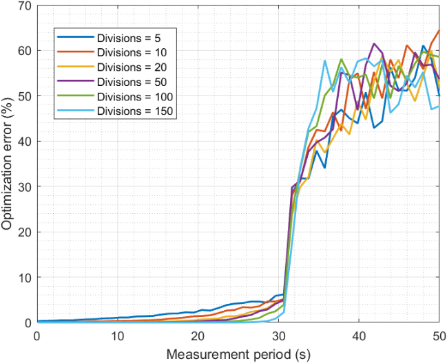
Additionally, also in this first region, simulations in which a higher number of divisions in the grid is considered present lower optimization errors. Because the proposed solution is discrete, as the number of divisions increases, the granularity of the K-means algorithm to find the optimum solution improves. Thus, errors go down. Anyway, errors below 5% are consistent with the expected performance from these optimization algorithms. We can conclude that the system behavior in this first region is good.
On the contrary, the convergence error for measurement periods above 32 seconds is very high (between 50% and 60%) and no difference is observed as the number of divisions, or the measurement period, evolves. That’s because, for devices moving at 500 km/h, measurement periods above 32 seconds are enough to go beyond the geographical limits of the area under study or to change their location to any point within the area with the same probability. In this situation, the optimization algorithms are fed with a problem with several possible solutions, as the initial data are not specific enough. The algorithms may then converge to any possible solution (almost randomly). This second region is not a useful working configuration and must be avoided.
Now, Fig. 6 shows the results for the second sub-experiment. The global optimization error is analyzed for different densities and speeds of devices. The measurement period was fixed at 1.5 seconds and the number of divisions within the grid was 25.
Figure 6.
Optimization error. Second sub-experiment: Results.
As explained above, for a given fixed measurement period, as the device speed increases, the number of possible target locations also increases. Therefore, uncertainty and convergence error grow. Errors, anyway, remain below 4%, which is consistent with the expected performance of the Adagrad algorithm.
This performance is, moreover, better than other optimization solutions for 6G networks reported in the literature. For example, resource optimization technologies based on Particle Swarm Optimization (PSO) algorithms, for interference mitigation in non-dense 6G verticals, report an error of around 1.8% for a device density of 100 devices per base station and device speeds close to 500 km/s [56]. In our proposal, the device density is four magnitude orders superior, whereas the optimization error is not even duplicated (it is around 3.2% under similar circumstances). This enhanced scalability is also significant for different speed values. For example, in previous PSO-based solutions [56], optimization error increases by approximately 1700% when speed changes from 150 km/h to 500 km/h. While in the proposed approach, the error only duplicates (again).
Besides, indeed, the convergence error increases as the device density increases. That is also an expected behavior, as optimization errors always increase as the number of variables to be considered grows. In this case, we can see the convergence error follows an exponential law we could be also intuited in the first region of Fig. 5. This exponential dependence is common in descent optimization algorithms. In general, then, we can conclude that the proposed optimization solution shows a good behavior.
Figure 7 presents the estimation error associated with the mobility diagnosis phase for different measurement periods. In this case, the number of divisions in the grid does not affect the results, as the grid is not part of the algorithm. We present the error in the speed estimation process and the trajectory calculation algorithm separately.
Qualitatively, all errors have the same behavior, although quantitatively the trajectory calculation is much more precise.
Figure 7.
Mobility diagnosis error. First sub-experiment: Results.
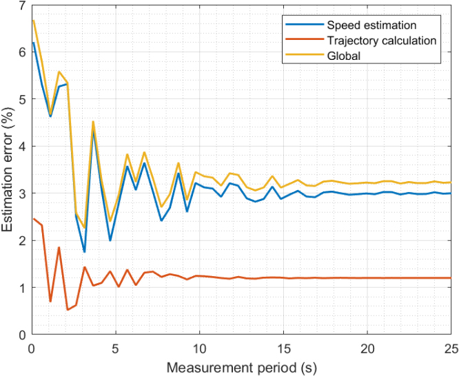
Figure 8.
Mobility diagnosis error. Second sub-experiment: Results.
For small measurement periods, radio signals are acquired for short periods too, and results are weak against some phenomena such as interferences, power absorption in the atmosphere, etc. which show up as fast and short bursts, but which can be relevant in short period. Then, errors then to be variable and almost random. As the measurement period increases, the impact of these phenomena is lower, and errors become stable. As trajectory estimation requires a much simpler processing, errors tend to be also lower. Thus, globally, the error in the mobility diagnosis phase is mainly caused by the speed estimation algorithm. The error, in any case, remains in the range of 3%, which is acceptable for a good optimization technology. Although the mobility diagnosis phase could benefit from large measurement periods, as this error is much lower than others (see Figs 5 and 9), it is preferable to reduce the measurement period and increase the estimation error in the speed estimation and reduce other errors in the system.
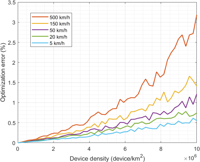
Figure 8 shows the evolution of the estimation error in the mobility diagnosis phase for different device densities and speeds. In this case, the error increases slowly but exponentially with the density and speed of the devices. The error is always below 2%, so the solution behaves well. But, as devices increase their speed and more devices are within the same area, complex effects in the radio spectrum may appear, such as interferences or frequency mixing. Those effects generate noise that, finally, affects the estimation process. This error can be reduced if the number of equations in the MSE minimization problems increases. But in that case, the processing delay would also be higher. Under any circumstances, a balance between precision and calculation delay must be achieved (so requirements of 6G dense vertical are met).
Finally, Fig. 9 shows the relative global prediction error associated with the proposed movement prediction model for different measurement periods and the number of divisions on the grid.
Figure 9.
Movement prediction error. First sub-experiment: Results.
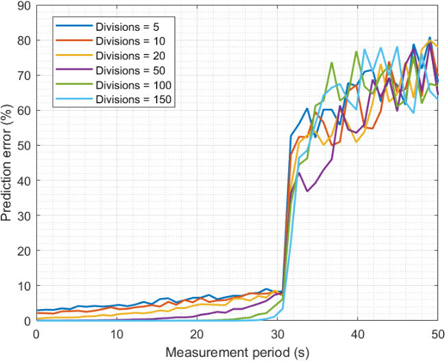
As can be seen, the evolution is similar to the one shown in Fig. 5. Although in this case, errors are significantly higher. Two regions are also observed in the graphic and explanations about the appearance of these two regions are identical to the one given before (Fig. 5). Once the measurement period is big enough so devices could move around the entire area under study, all locations, are possible future locations and errors increase. This region has no good behavior and it is not a valid working configuration. In the valid working region, the error may reach 10%, still a good value but higher than the ones obtained in previous analyses. So, it is preferred to choose the configuration that reduces this estimation error, rather than other errors such as the estimation error in the mobility diagnosis phase.
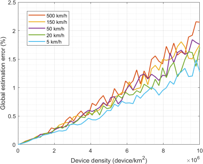
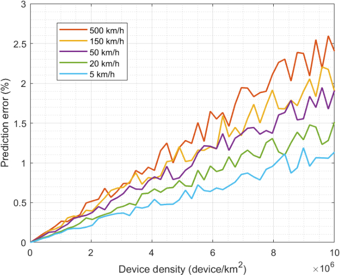
Figure 10 shows the evolution of the prediction error for different densities and speeds of devices. As said above (Fig. 6), for a given fixed measurement period, as the device speed increases, the number of possible target locations also increases. So, uncertainty and convergence error increase (as also shown in Fig. 10). In this case, however, the prediction error increases (almost) linearly with the device density. In general, movement prediction for each device is independent (so the device density does not affect), but when all independent predictions are aggregated, errors are also accumulated. Anyway, the errors are low (below 3%) and the choreographed movement prediction algorithm shows good behavior.
Compared to other traditional movement prediction techniques, based on standalone Markov models, prediction error is much lower. In previous proposals where simple Markov chains are employed [52] prediction error is always above 20%. This error can be reduced when enough historical data are considered, and more elaborate Hidden Markov Models are used [56]. In those cases, long-term reported prediction error is around 10%, but for some very specific configurations, can reduce up to 3.5%. Thus, in the worst case, the proposed solution improves the performance of previously reported mechanisms in the literature, at least around 15%. Other techniques, based on artificial intelligence, show better performance [51]. But they require large processing delays, so can not operate under high mobility conditions (and they are not a valid approach for 6G dense verticals).
Figure 10.
Prediction error. Second sub-experiment: Results.
On the other hand, once proved the proposed solution has a good mathematical behavior, it is essential to analyze the performance of the proposed solution.
First, Fig. 11 shows the processing delay required by the proposed management solution for different device densities and numbers of divisions in the geographical grid. As can be seen (the vertical axis is logarithmic), the processing delay evolves slowly but linearly as the device density increases. That was expected as mobility diagnosis and movement prediction must be performed for every single device within the vertical range. But because the proposed solution is choreographed, not all base stations must analyze all devices, but only those within their coverage area. Then, the rate of increase is slower in the processing delay than in the number of devices deployed in the dense vertical.
Figure 11.
Experimental results: Processing delay.

However, the impact of the number of divisions in the geographical grid is more relevant. As the proposed solution analyzes several times every possible location within the grid, the processing delay increases quickly when the number of divisions in the grid increases. But even for 150 divisions (a large number considering we are only analyzing 20 square kilometers and devices show ultra-high speed), the processing delay is still around 4 seconds. Considering that the measurement period must be, for sure, lower than the processing delay and higher than the time needed for a device to cross the entire area under study, the proposed solution is still useful in verticals with an effective area of only one square kilometer and devices moving 500 km/h. Considering the coverage areas in 6G networks (only one base station may cover up to twenty kilometers), these values are good results. These results then confirm that the proposed approach is actually valid for dense 6G vertical with high-speed requirements.
Finally, Fig. 12 shows the management and optimization capacity of the proposed technology. Results are normalized to amplify the differences between the different configurations. Results are shown for different device densities and numbers of divisions in the geographical grid. Furthermore, results are compared to state-of-the-art technologies (FIFO queues [55]).
Although intelligent approaches are even unable to converge in 6G dense scenarios [31] (and they do not generate any valid result), FIFO queues [55] might be implemented in 6G verticals. But, as can be seen, for all network configurations and device densities, the proposed solution is able to optimize QoS better than this previous and traditional approach. In fact, the resource consumption required to achieve a given QoS reduces (on average) 12% compared to state-of-the-art technologies. However, as device density increases, this difference increases and reaches up to 40%. In general, FIFO queues are very efficient in scenarios where the probability of congestion and/or lack of network resources is a very improbable situation (such, for example, in traditional telephone networks). But as the density of the verticals increases, congestion becomes more probable. Our proposed solution fights against this situation through several prediction and optimization stages: reducing resource consumption and increasing the real efficiency. Thus, the evolution is exponential but slow. However, traditional FIFO queues can only address this problem by increasing the network resources. Because of that, exponential growth is very fast, and it is more relevant as the device density is higher.
Figure 12.
Experimental results: Management and optimization capacity.
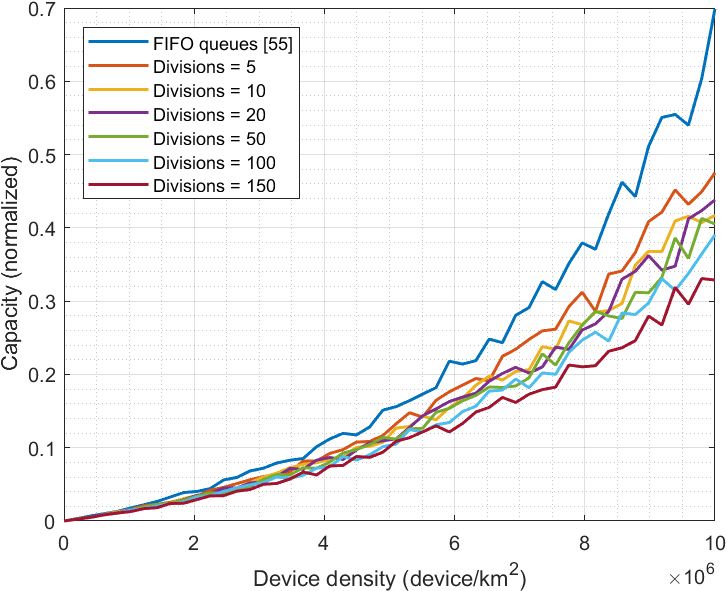
Differences between different configurations (number of divisions) of the proposed management technology are less significant and only achieve 10% when larger numbers of divisions (150) are considered. For these large values, since the optimization algorithms are more precise, a better distribution of resources and a more efficient QoS management are expected. The required resources increase exponentially as the device increases, but that is the expected behavior in mobile networks. Management and optimization solutions are only aimed at reducing the increasing rate, as shown in Fig. 12.
It is also interesting to analyze the left side of Fig. 12. As can be seen, for sparse networks (low device density), differences between the traditional approaches (FIFO queues) and the proposed solution are not as relevant as in 6G dense verticals. In that context, the benefit of this new mechanism might not be worth the computational overhead introduced. And common schemes would be enough. Then, future 6G network should include mechanisms to adapt its behavior to the vertical density at each moment.
Therefore, we can conclude that the proposed solution allows for an efficient QoS management in dense 6G verticals with high mobility requirements.
6.Conclusions
In this paper, we propose a choreographed QoS management solution, where 6G base stations predict the evolution of verticals at real-time, and run a lightweight choreographed optimization algorithm in advance, so they can manage the resource consumption and ensure all devices get the required QoS. Prediction mechanism includes mobility models (Markov, Bayesian, etc.) and models for time-variant communication channels. In addition, a traffic prediction solution is also considered to explore the QoS achieved in advance. The optimization algorithm calculates an efficient resource distribution based on the predicted future vertical situation predicted, so devices achieve the expected QoS according to the proposed traffic models.
The results of the experimental validation showed that the proposed solution has a good mathematical behavior, where the optimization errors are 4%. Additionally, the solution has a limited computational cost, and it is able to work even in verticals with an effective area of only one square kilometer and devices moving 500 km/h. Finally, the solution optimizes and manages QoS efficiently and reduces up to 12% (sustainable) of the resource consumption compared to common traditional approaches.
Future work will analyze the performance of the solutions with devices with free movement (not only with closed curves). Additionally, scenarios with devices densities beyond extreme will be considered. And studies about the verisimilitude of simulations will be provided. Moreover, enhanced simulation methods will be considered too, such as techniques based on the maximum verisimilitude algorithm. So, results more statically significant can be obtained. In addition, the performance of the solution in real distributed machines will be studied. Additionally, the impact of new radio signal control technologies, such as reconfigurable intelligent surfaces, will be considered. Finally, other unsupervised optimization techniques to solve the global and resulting QoS optimization problem will be considered and studied, including nature-inspired algorithms, as well as their compatibility with high mobility requirements in 6G dense verticals.
Acknowledgments
The publication is produced within the framework of Ramón Alcarria y Borja Bordel’s research projects on the occasion of their stay at Argonne Labs (José Castillejo’s 2021 grant). This work is supported by the Spanish Ministry of Science, Innovation and Universities through the COGNOS project (PID2019-105484RB-I00).
References
[1] | Zhang Z, Xiao Y, Ma Z, Xiao M, Ding Z, Lei X, et al. 6G wireless networks: Vision, requirements, architecture, and key technologies. IEEE Vehicular Technology Magazine. (2019) ; 14: (3): 28-41. |
[2] | Chen S, Liang YC, Sun S, Kang S, Cheng W, Peng M. Vision, requirements, and technology trend of 6G: How to tackle the challenges of system coverage, capacity, user data-rate and movement speed. IEEE Wireless Communications. (2020) ; 27: (2): 218-228. |
[3] | Bordel Sánchez B, Alcarria R, Robles T. Managing wireless communications for emergency situations in urban environments through cyber-physical systems and 5G technologies. Electronics. (2020) ; 9: (9): 1524. |
[4] | Bordel B, Alcarria R, Robles T. An Optimization Algorithm for the Efficient Distribution of Resources in 6G Verticals. In World Conference on Information Systems and Technologies; Springer, Cham; (2022) May. pp. 103-114. |
[5] | Matinmikko-Blue M, Yrjölä S, Ahokangas P. Moving from 5G in verticals to sustainable 6G: Business, regulatory and technical research prospects. In International Conference on Cognitive Radio Oriented Wireless Networks; Springer, Cham; (2020) Nov. pp. 176-191. |
[6] | Bordel B, Alcarria R, Sánchez-de-Rivera D, Sánchez Á. An inter-slice management solution for future virtualization-based 5G systems. In International Conference on Advanced Information Networking and Applications; Springer, Cham; (2019) March. pp. 1059-1070. |
[7] | Sutton GJ, Zeng J, Liu R, Ni W, Nguyen DN, Jayawickrama BA, Lv T. Enabling technologies for ultra-reliable and low latency communications: From PHY and MAC layer perspectives. IEEE Communications Surveys & Tutorials. (2019) ; 21: (3): 2488-2524. |
[8] | Li H, Wang G, Lu J, Kiritsis D. Cognitive twin construction for system of systems operation based on semantic integration and high-level architecture. Integrated Computer-Aided Engineering. (2022) ; 29: (3): 277-295. |
[9] | Wu H, He F, Duan Y, Yan X. Perceptual metric-guided human image generation. Integrated Computer-Aided Engineering. (2022) ; 29: (2): 141-151. |
[10] | Siddique N, Adeli H. Nature inspired computing: An overview and some future directions. Cognitive Computation. (2015) ; 7: : 706-714. |
[11] | Yang H, Alphones A, Xiong Z, Niyato D, Zhao J, Wu K. Artificial-intelligence-enabled intelligent 6G networks. IEEE Network. (2020) ; 34: (6): 272-280. |
[12] | Siddique N, Adeli H. Spiral dynamics algorithm. International Journal on Artificial Intelligence Tools. (2014) ; 23: (6): 1430001. |
[13] | Akhand MAH, Ayon SI, Shahriyar SA, Siddique N, Adeli H. Discrete spider monkey optimization for travelling salesman problem. Applied Soft Computing. (2020) ; 86: : 105887. |
[14] | Xue Y, Zhu H, Neri F. A self-adaptive multi-objective feature selection approach for classification problems. Integrated Computer-Aided Engineering. (2022) ; 29: (1): 3-21. |
[15] | Yang Z, Chen M, Wong KK, Poor HV, Cui S. Federated learning for 6G: Applications, challenges, and opportunities. Engineering. (2021) ; 8: : 33-41. |
[16] | Fan P, Zhao J, Chih-Lin I. 5G high mobility wireless communications: Challenges and solutions. China Communications. (2016) ; 13: (2): 1-13. |
[17] | Bordel B, Alcarria R, Chung J, Kettimuthu R, Robles T, Armuelles I. Towards Fully Secure 5G Ultra-Low Latency Communications: A Cost-Security Functions Analysis. Computers, Materials & Continua. (2023) ; 75: (1). |
[18] | Rappaport TS, Xing Y, Kanhere O, Ju S, Madanayake A, Mandal S, et al. Wireless communications and applications above 100 GHz: Opportunities and challenges for 6G and beyond. IEEE Access. (2019) ; 7: : 78729-78757. |
[19] | Bordel B, Alcarria R, Martín D, Sánchez-de-Rivera D. An agent-based method for trust graph calculation in resource constrained environments. Integrated Computer-Aided Engineering. (2020) ; 27: (1): 37-56. |
[20] | Dong R, She C, Hardjawana W, Li Y, Vucetic B. Deep learning for radio resource allocation with diverse quality-of-service requirements in 5G. IEEE Transactions on Wireless Communications. (2020) ; 20: (4): 2309-2324. |
[21] | Sun C, She C, Yang C, Quek TQ, Li Y, Vucetic B. Optimizing resource allocation in the short blocklength regime for ultra-reliable and low-latency communications. IEEE Transactions on Wireless Communications. (2018) ; 18: (1): 402-415. |
[22] | Sun H, Chen X, Shi Q, Hong M, Fu X, Sidiropoulos ND. Learning to optimize: Training deep neural networks for interference management. IEEE Transactions on Signal Processing. (2018) ; 66: (20): 5438-5453. |
[23] | Hu Y, Ozmen M, Gursoy MC, Schmeink A. Optimal power allocation for QoS-constrained downlink multi-user networks in the finite blocklength regime. IEEE Transactions on Wireless Communications. (2018) ; 17: (9): 5827-5840. |
[24] | Banchs A, Fiore M, Garcia-Saavedra A, Gramaglia M. Network intelligence in 6G: Challenges and opportunities. In Proceedings of the 16th ACM Workshop on Mobility in the Evolving Internet Architecture. (2021) Oct. pp. 7-12. |
[25] | Lydia A, Francis S. Adagrad – an optimizer for stochastic gradient descent. Int. J. Inf. Comput. Sci. (2019) ; 6: (5): 566-568. |
[26] | Peng Q, Walid A, Hwang J, Low SH. Multipath TCP: Analysis, design, and implementation. IEEE/ACM Transactions on Networking. (2014) ; 24: (1): 596-609. |
[27] | Bozdogan H. Model selection and Akaike’s information criterion (AIC): The general theory and its analytical extensions. Psychometrika. (1987) ; 52: (3): 345-370. |
[28] | Jeon YS, Hong SN, Lee N. Supervised-learning-aided communication framework for MIMO systems with low-resolution ADCs. IEEE Transactions on Vehicular Technology. (2018) ; 67: (8): 7299-7313. |
[29] | Adediran YA, Lasisi H, Okedere OB. Interference management techniques in cellular networks: A review. Cogent Engineering. (2017) ; 4: (1): 1294133. |
[30] | Mahmood MR, Matin MA, Sarigiannidis P, Goudos SK. A Comprehensive Review on Artificial Intelligence/Machine Learning Algorithms for Empowering the Future IoT Toward 6G Era. IEEE Access. (2022) ; 10: : 87535-87562. |
[31] | Rekkas VP, Sotiroudis S, Sarigiannidis P, Wan S, Karagiannidis GK, Goudos SK. Machine Learning in Beyond 5G/6G Networks-State-of-the-Art and Future Trends. Electronics. (2021) ; 10: (22): 2786. |
[32] | Bordel B, Alcarria R, Robles T, Sanchez-de-Rivera D. Service management in virtualization-based architectures for 5G systems with network slicing. Integrated Computer-Aided Engineering. (2020) ; 27: (1): 77-99. |
[33] | Aljiznawi RA, Alkhazaali NH, Jabbar SQ, Kadhim DJ. Quality of service (qos) for 5g networks. International Journal of Future Computer and Communication. (2017) ; 6: (1): 27. |
[34] | Morabito AF, Di Donato L, Isernia T. Orbital angular momentum antennas: Understanding actual possibilities through the aperture antennas theory. IEEE Antennas and Propagation Magazine. (2018) ; 60: (2): 59-67. |
[35] | Al-Shaikhli A, Esmailpour A. Quality of Service management in 5G broadband converged networks. In 2015 36th IEEE Sarnoff Symposium; IEEE; (2015) Sept. pp. 56-61. |
[36] | Irazabal M, Lopez-Aguilera E, Demirkol I. Active queue management as quality of service enabler for 5G networks. In 2019 European Conference on Networks and Communications (EuCNC); IEEE; (2019) June. pp. 421-426. |
[37] | Fan P, Zhao J, Chih-Lin I. 5G high mobility wireless communications: Challenges and solutions. China Communications. (2016) ; 13: (2): 1-13. |
[38] | Angjo J, Shayea I, Ergen M, Mohamad H, Alhammadi A, Daradkeh YI. Handover management of drones in future mobile networks: 6G technologies. IEEE Access. (2021) ; 9: : 12803-12823. |
[39] | Jain A, Lopez-Aguilera E, Demirkol I. Are mobility management solutions ready for 5G and beyond? Computer Communications. (2020) ; 161: : 50-75. |
[40] | Li Y, Li Q, Zhang Z, Baig G, Qiu L, Lu S. Beyond 5g: Reliable extreme mobility management. In Proceedings of the Annual conference of the ACM Special Interest Group on Data Communication on the applications, technologies, architectures, and protocols for computer communication; ACM; (2020) July. pp. 344-358. |
[41] | Aljeri N, Boukerche A. Mobility management in 5G-enabled vehicular networks: models, protocols, and classification. ACM Computing Surveys (CSUR). (2020) ; 53: (5): 1-35. |
[42] | Giust F, Cominardi L, Bernardos CJ. Distributed mobility management for future 5G networks: Overview and analysis of existing approaches. IEEE Communications Magazine. (2015) ; 53: (1): 142-149. |
[43] | Zhang S, Liu J, Guo H, Qi M, Kato N. Envisioning device-to-device communications in 6G. IEEE Network. (2020) ; 34: (3): 86-91. |
[44] | Heinonen J, Korja P, Partti T, Flinck H, Pöyhönen P. Mobility management enhancements for 5G low latency services. In 2016 IEEE International Conference on Communications Workshops (ICC); IEEE; (2016) May. pp. 68-73. |
[45] | Calabuig D, Barmpounakis S, Gimenez S, Kousaridas A, Lakshmana TR, Lorca J, Maternia M. Resource and mobility management in the network layer of 5G cellular ultra-dense networks. IEEE Communications Magazine. (2017) ; 55: (6): 162-169. |
[46] | Chen S, Qin F, Hu B, Li X, Chen Z. User-centric ultra-dense networks for 5G: Challenges, methodologies, and directions. IEEE Wireless Communications. (2016) ; 23: (2): 78-85. |
[47] | Semiari O, Saad W, Bennis M, Maham B. Caching meets millimeter wave communications for enhanced mobility management in 5G networks. IEEE Transactions on Wireless Communications. (2017) ; 17: (2): 779-793. |
[48] | Giordani M, Zorzi M. Non-terrestrial networks in the 6G era: Challenges and opportunities. IEEE Network. (2020) ; 35: (2): 244-251. |
[49] | Araniti G, Iera A, Pizzi S, Rinaldi F. Toward 6g non-terrestrial networks. IEEE Network. (2021) ; 36: (1): 113-120. |
[50] | Hou J, Zhao H, Zhao X, Zhang J. Predicting mobile users’ behaviors and locations using dynamic Bayesian networks. Journal of Management Analytics. (2016) ; 3: (3): 191-205. |
[51] | Hotson G, Smith RJ, Rouse AG, Schieber MH, Thakor NV, Wester BA. High precision neural decoding of complex movement trajectories using recursive Bayesian estimation with dynamic movement primitives. IEEE Robotics and Automation Letters. (2016) ; 1: (2): 676-683. |
[52] | Asahara A, Maruyama K, Sato A, Seto K. Pedestrian-movement prediction based on mixed Markov-chain model. In Proceedings of the 19th ACM SIGSPATIAL International Conference on Advances in Geographic Information Systems; ACM; (2011) Nov. pp. 25-33. |
[53] | Bello P. Characterization of randomly time-variant linear channels. IEEE transactions on Communications Systems. (1963) ; 11: (4): 360-393. |
[54] | Li X, Deng S, Li L, Jiang Y. Outlier detection based on robust mahalanobis distance and its application. Open Journal of Statistics. (2019) ; 9: (1): 15-26. |
[55] | Tekinay S, Jabbari B. A measurement-based prioritization scheme for handovers in mobile cellular networks. IEEE Journal on selected Areas in Communications. (1992) ; 10: (8): 1343-1350. |
[56] | Bordel B, Alcarria R, Robles T. Interferenceless coexistence of 6G networks and scientific instruments in the K a-band. Expert Systems. (2023) ; e13369. |
[57] | Si H, Wang Y, Yuan J, Shan X. Mobility prediction in cellular network using hidden markov model. In 2010 7th IEEE Consumer Communications and Networking Conference; IEEE; (2010) January. pp. 1-5. |

