
Machine Learning-Based Classification of Parkinson’s Disease Patients Using Speech Biomarkers
Abstract
Background:
Parkinson’s disease (PD) is the most prevalent neurodegenerative movement disorder and a growing health concern in demographically aging societies. The prevalence of PD among individuals over the age of 60 and 80 years has been reported to range between 1% and 4%. A timely diagnosis of PD is desirable, even though it poses challenges to medical systems.
Objective:
This study aimed to classify PD and healthy controls based on the analysis of voice records at different frequencies using machine learning (ML) algorithms.
Methods:
The voices of 252 individuals aged 33 to 87 years were recorded. Based on the voice record data, ML algorithms can distinguish PD patients and healthy controls. One binary decision variable was associated with 756 instances and 754 attributes. Voice records data were analyzed through supervised ML algorithms and pipelines. A 10-fold cross-validation method was used to validate models.
Results:
In the classification of PD patients, ML models were performed with 84.21 accuracy, 93 precision, 89 Sensitivity, 89 F1-scores, and 87 AUC. The pipeline performance improved to accuracy: 85.09, precision: 92, Sensitivity:91, F1-score: 89, and AUC: 90. The Pipeline methods improved the performance of classifying PD from voice record.
Conclusions:
Our study demonstrated that ML classifiers and pipelines can classify PD patients based on speech biomarkers. It was found that pipelines were more effective at selecting the most relevant features from high-dimensional data and at accurately classifying PD patients and healthy controls. This approach can therefore be used for early diagnosis of initial forms of PD.
INTRODUCTION
Parkinson’s disease (PD) is the second most common neurodegenerative disease after Alzheimer’s disease [1]. The prevalence of PD is 1% among people over the age of 60 years and 4% among those over the age of 80 years [2]. Approximately one to two people out of every 1,000 suffer from PD [3]. The number of PD patients is increasing in parallel with the increase in the elderly population. Globally, the number of PD patients has doubled between 1990 and 2015, with approximately 6.2 million individuals affected [4]. Since 1990, the age-standardized prevalence rate (ASR) increased by 21.7% [5].
PD is a progressive neurodegenerative disorder characterized by motor impairment [6] and by the presence of bradykinesia, rest tremors, rigidity, as well as changes in posture and gait. Disturbances in motor function led to progressive disability, impairment of daily activities, and worsening in quality of life. Nearly all patients with PD suffer from a variety of non-motor symptoms (NMS), such as hyposmia, constipation, urinary dysfunction, orthostatic hypotension, memory loss, depression, pain, and sleep disturbances [7]. PD most commonly affects elderly people, although cases of young patients are not uncommon.
Voice problems usually are among the earliest symptoms. They are followed by other disorders occurring later and more gradually, such as prosody, difficulties in word articulation, and fluency. Most PD patients have hoarse voice quality, soft voice, breathiness monotone, and imprecise articulation which may affect their oral communication [8, 9]. A well-integrated speech needs normal respiration, phonation, and articulation. The breakdown of those subsystems and their combination results in speech disorders [10, 11].
Early detection and treatment are important for patients with PD. There is no reliable diagnostic test currently, and PD identification is based primarily on clinical criteria [12–14]. Traditionally, the early diagnosis of PD is based on interviews with the patient followed by careful neurological examinations [15, 16]. So far there is no intelligent computing approach collecting different symptoms for speeding up the diagnosis of the disease. Telediagnosis and telemonitoring approaches recently introduced represent non-intelligent methods for diagnosing PD and these systems are unable to solve complex problems based on data-intensive learning. It could therefore be useful to develop automated systems to help in the early diagnosis of PD.
Acoustic testing can help to identify PD because patients may have some subtle irregularities in their speech that might not be perceived by an audience. Recent studies have developed methods for analyzing and classifying the speech of PD patients [17, 18]. Machine learning (ML) has been extensively used in a variety of applications requiring data collected in some specific format. Data-intensive problems can be solved using statistical models and learning-based solutions. Healthcare applications have also successfully adopted these approaches [15, 19, 20].
Studies published in the area of PD diagnosis have mainly investigated the impact of a particular subset of features on the accurate diagnosis of PD [21]. A few review articles have examined the ML algorithm performance, whereas others have examined heuristic and meta-heuristic algorithms’ influence on the accurate diagnosis of PD [22–24]. ML algorithms generally perform less well when progressively more features/dimensions are fed to them [25]. Data collected from PD patients consists of hundreds of dimensions, making it impossible to use ML algorithms to classify PD. Hence, for an accurate diagnosis of PD, problems should be analyzed with high dimensionality.
The primary objective of this paper was to utilize supervised ML techniques to classify PD patients based on speech recording data. Our work was divided into two steps. In the first step, we evaluated supervised ML classifiers that could identify PD patients. In the second step, we applied the feature selection technique from the model (support vector machine) and then classified PD patients based on those selective features with the combination of ML machine learning algorithms that we have identified in the first part. To facilitate the selection and classification of features, a pipeline approach was developed. To identify the most effective model, we compared traditional classifiers and pipeline performance in the results section.
MATERIALS AND METHODS
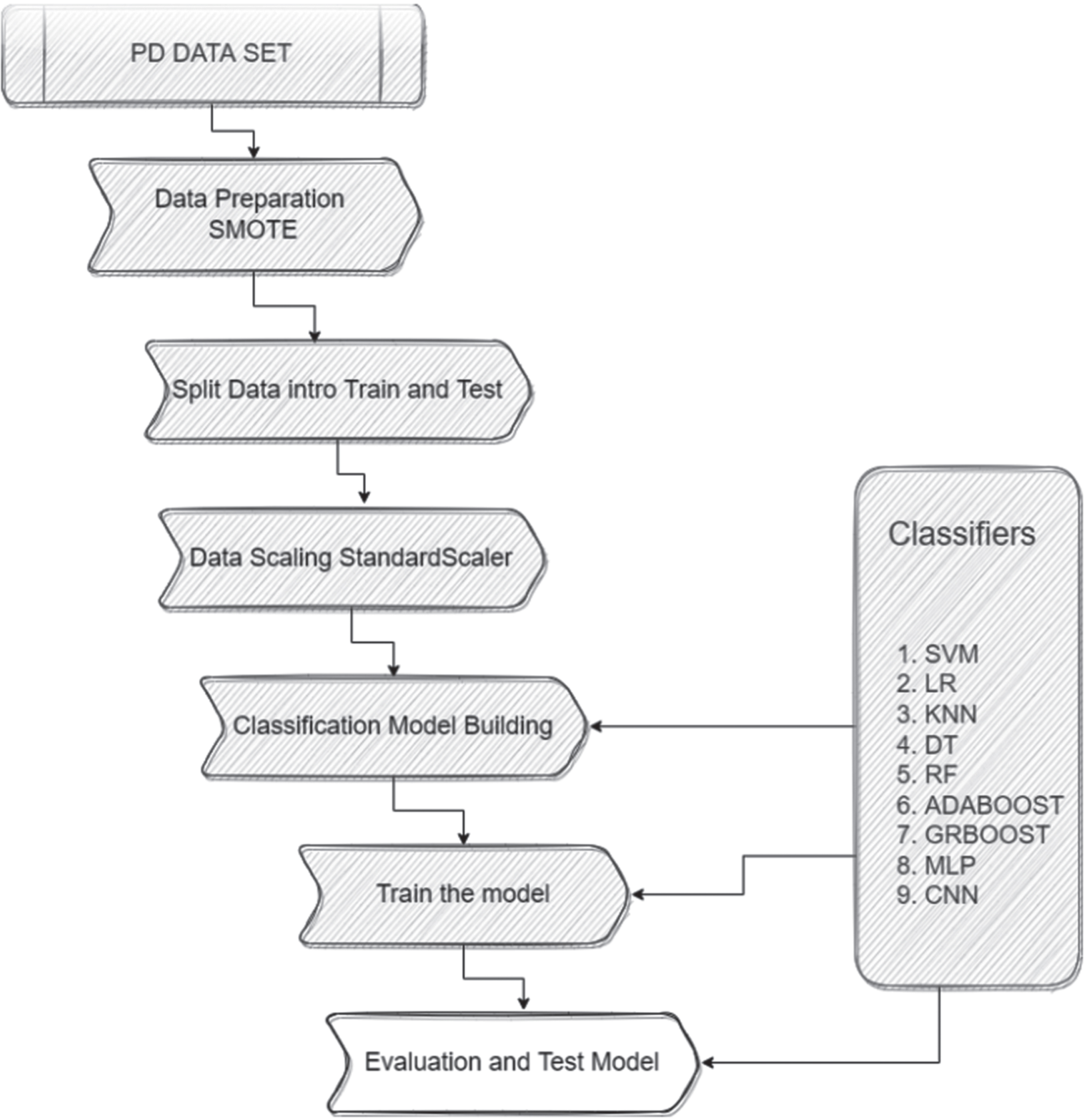
The graphical representation of work is in Fig. 1. Below sections we briefly described all materials and methods used in this work.
Fig. 1
Framework to classify Parkinson’s disease.
Data set description
The data used in this study was collected by the Department of Neurology at Istanbul University’s Cerrahpaşa [26]. Overall, 252 individuals were surveyed (130 males and 122 females), and each subject had three records. There were 756 instances and 754 attributes, and one binary decision variable. The sample included 188 patients with PD (107 men and 81 women), aged between 33 and 87 years and their mean age 65.1±10.9. The 64 healthy individuals were 23 men and 41 women, and their ages ranged from 41 to 82 years with the mean of 61.1±8.9. The microphone used was set to 44.1 kHz during the data collection process. They shared this dataset to the machine learning repository UCI (University of California Irvine) [27]. Students, educators, and researchers throughout the world have access to UCI databases, domain theories, and data generators which are used in machine learning applications.
In the dataset description, there was no mention of the duration and stage of the patients’ disease. However, in their more recent work [28], the authors estimated the severity of PD using the same voice recording dataset, employing the motor Unified Parkinson’s Disease Rating Scale (UPDRS) score as the evaluation metric. In this study, UPDRS scores were available for 86 PD patients (comprising 49 males and 37 females) out of the total 188 participants in the study. The mean duration since PD diagnosis was found to be 5.55 years with a standard deviation of 4.72 years. When we further stratify the data by gender, we find that males had an average diagnosis duration of 5.12 years with a standard deviation of 4.23 years, while females had an average diagnosis duration of 6.13 years with a standard deviation of 5.31 years. Upon a thorough examination of this work, we now understand that the sample primarily consisted of early-stage PD patients.
After the physician’s examination, three repetitions of sustained phonation of the vowel “a” were recorded from each subject. A variety of speech signal processing algorithms have been applied to the recordings of PD patients to extract clinically useful information for assessing PD symptoms. These included Time-Frequency Features, Mel Frequency Cepstral Coefficients (MFCCs), Wavelet Transform based Features, Vocal Fold Features, and Tunable Q-factor wavelet transform (TWQT) features. “Baseline features” include jitter, shimmer, recurrence period density entropy (RPDE), fundamental frequency parameters, Detrended Fluctuation Analysis (DFA), harmonicity parameters, and Pitch Period Entropy (PPE) [22–24, 29, 30]. The data set contained 756 recorded observations (rows), and 755 features (columns), of which 752 have real values, 1 has values between 0 and 2, and two have binary values. The last column of this data set represents a binary value indicating PD or health status, also known as decision variables. ML classifiers can use class variables to extract pertinent information on PD patients. In Table 1 an overview of each attribute of the dataset.
Table 1
Parkinson’s disease speech biomarkers data set descriptions
| Features Name | Description | No. of Columns | Column Range |
| ID | Numeric | 1 | Col_1 |
| Gender | Binary | 1 | Col_2 |
| Baseline Features | Real | 21 | Col_3 to Col_23 |
| Intensity Parameters | Real | 3 | Col_24 to Col_26 |
| Formant Frequencies | Real | 4 | Col_27 to Col_30 |
| Bandwidth Parameters | Real | 4 | col_31 to Col_34 |
| Vocal Fold | Real | 22 | Col_35 to Col_56 |
| MFCC | Real | 84 | Col_57 to Col_140 |
| Wavelet Features | Real | 182 | Col_141 to Col_322 |
| TQWT Features | Real | 432 | Col_323 to Col_754 |
| Class (Depended Variable) | Binary | 1 | Col_755 |
ID, Identity; MFCC, Mel Frequency Cepstral Coefficients; TQWT, Tunable Q-factor wavelet transform.
Data preparation
The data set selected for analysis is a secondary and processed set. The data set does not contain any missing or null values. Therefore, no data processing performs to deal with missing and/or null values. To classify PD from this dataset, we split the data into train and test, balanced the dependent value, and selected the features according to the model’s requirements. Data preparation details are discussed in this section.
Splitting data
ML classifiers provide biased results (overfitting) when trained with a complete data set without testing with unseen data. To overcome this problem, a cross-validation model evaluation method usually recommended when developing a ML classification model was used. Data were divided into subsets based on pre-defined ratios, and each subset is used to train and evaluate a ML classification model. To generalize the performance of the model concerning classification accuracy, the average error rate is calculated. A standard procedure uses 70% of the data for training and 30% for testing. ML classifiers are trained on the training data. These classifiers were evaluated and validated on the test set. It is indeed challenging to split medical data. The dataset consists of 756 records of 252 patients. Each patient has three observations. In the case of a random split, the same patient records can appear on both the train and test sets. To avoid this scenario, the data set is sorted by the number of patients. The ID value is unique to each patient. Before splitting, the patient’s position was randomized so that there is a random patient record on the train set, not from the serial. There are 188 PD patients and 64 healthy or control. 80% (151 PD and 51 healthy) of patients in each group are divided into train sets, while 20% (37 PD and 13 healthy) are test sets.
Balancing data
This data set is balanced by gender (males:130 and females:122). 564 (188 X 3) of the records are from PD patients and 192 records (64 X 3) are from healthy patients, so the variable “class” is not balanced. Table 2 indicates the number of male and female PD and subjects examined. A SMOTE: synthetic minority over-sampling technique [31] is applied to the target value “class” to balance the data set. In SMOTE, examples that are close to the feature space are selected, a line is drawn between them, and a new sample is drawn along the line.
Table 2
Number of male and female subjects [Parkinson’s disease (PD) and healthy individuals] examined in the present study
| Gender | Class | Number |
| Male | Healthy | 23 |
| PD | 107 | |
| Female | Healthy | 41 |
| PD | 82 |
First, a random example from the minority class is picked. For each example, k nearest neighbors is found (typically k = 5). Based on the selected neighbor and a randomly chosen to point between them in feature space, a synthetic example is created.
Feature scaling
Feature scaling is a preprocessing step in data analysis that normalizes features to a particular range without affecting the essence of the data. ML classifier’s time consumption can also be reduced by feature scaling. Sklearn’s Standard Scaler [32] is used to scale the values in the data set to address the problem of sparsity in the data set, as well as to accelerate the calculations of ML classifiers. Standard Scaler removes the mean and scales to unit variance. A standard score of samples a is calculated according to the formula s = (a-u)/c. where u represents the mean of the training samples or zero if with mean = false and c represents the standard deviation of the training samples or one if with std = false. Based on the samples in the training set, each feature is centered and scaled independently. Mean and standard deviation are then stored for later use with transform.
Model design
The ‘class’ column represents the target variable (y). The remaining columns are inputs (x). Supervised learning algorithms were used since the results of this task were already available. Support Vector Machine (SVM), Logistic Regression classifier (LR), K-Nearest Neighbors (KNN), Decision Tree (DT), Random Forest classifier (RF), AdaBoost and Gradient Boosting and Multi-Layer Perception (MLP) are the classifier algorithms used in this work. The dataset has 756 features. All the features are not relevant to the classification of PD patients, and it is difficult to handle more input features. To minimize the number of input features and find the more relevant features to the target value the feature selection technique was applied. The features selected from the model technique were used. The pipelines were developed on selected features.
Logistic regression classifier (LR)
LR is a simple and efficient algorithm for binary and linear classification problems (the target is categorical). An LR uses a logistic function to model a binary output variable [33]. LR employs a nonlinear log transformation and does not require linear relationships between inputs and outputs. In the equation, x is the input variable.
LR parameter setting
The parameters are penalty = ‘L1’, solver = ‘liblinear’, and random_state = 0 and tol = 1e–6. The rest of the parameters are set to default. Due to the size of the dataset, the solver chose to use ‘liblinear’. We set the penalty ‘L1’ as the dataset has many features and ‘L1’ regularization. The model was also validated with 10-fold cross-validation.
Support vector machine (SVM)
The SVM algorithm is to find a hyperplane in an N-dimensional space. Many possible hyperplanes can be chosen to separate the two classes of data points. To find the maximum margin, we must find the maximum distance between points of both classes. Hyperplanes serve as decision boundaries that help to classify the data points. By increasing the margin distance, future data points can also be classified with greater confidence. The data points on either side of the hyperplane can be assigned to different classes. The dimensions of the hyperplane are also determined by the number of features. In the case of two input features, the hyperplane is just a line. The hyperplane becomes two-dimensional if there are three input features. If there are more than three features, it becomes hard.
SVM parameter setting
Linear kernel chose to classify with SVM, Regularization parameter is set C = 0.01 and other parameters set by default. To validate the model 10-fold cross-validation was also performed.
K-Nearest neighbors (KNN)
A supervised machine learning algorithm is used to solve classification and regression problems. Select K neighbors (K = 5) and calculate the Euclidean distance (ED):
KNN parameter setting
Number of neighbors K = 5, uniform weights, algorithm, and leaf size is set as default value.
Decision Tree
The decision tree (DT) is a non-parametric supervised learning technique used for classification and regression. We are attempting to develop a model that predicts the value of a target variable by learning simple decision rules based on the characteristics of the data. In general, a tree can be considered as an approximation of a constant piecewise function.
DT parameter setting
The classification criteria used criterion=‘gini’, mathematically H (Qm) = ∑kpmk (1 - pmk). The ‘best’ splitter is used to split the node. Minimum samples split and leaf is set as 2 and 1 respectively.
Random forest classifier
Random forests (RF) consist of several decision trees that predict the outcome. In a random forest classification technique, a class is selected based on the input information. The random forest will determine whose class has the highest number of values once all trees have concluded.
RF parameter setting
The RF model was built using 300 estimators. Was control the randomness of bootstrapping and sample selection to build a tree.
AdaBoost classifier
AdaBoost is a technique for ensemble learning. A classifier and an additional copy of the classifier are fitted to the original dataset. By adjusting the weights of incorrectly classified instances, subsequent classifiers can focus more on difficult cases.
AdaBoost parameter setting
Our model is built using 100 estimators and randomness control, like the RF model.
Gradient boosting classifier
It is interesting to note that Gradient Boosting works by fitting a new predictor to the residual errors of the previous predictor rather than fitting it to the data at each iteration. A major objective of gradient boosting is to reduce the errors of its predecessor by reducing errors its predecessor.
Gradient boosting parameter setting
The model is constructed by setting the number estimator to 100, the learning rate to 1, and the maximum depth to 1. In addition, we control the randomness of the model.
Multi-Layer Perception
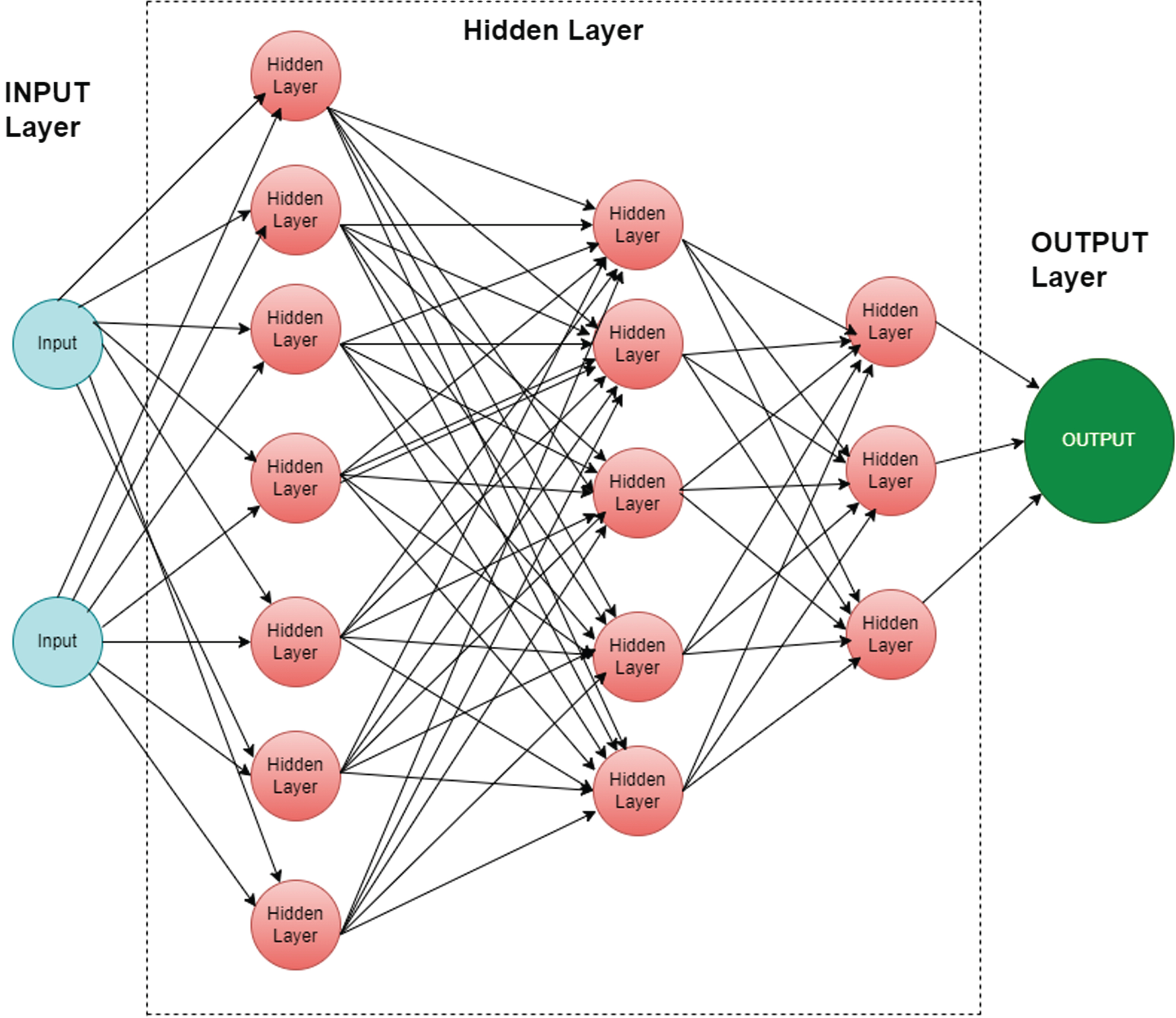
Multi-Layer Perception (MLP) Classifier stands for MLP classifier. It is a feedforward artificial neural network model that maps inputs into outputs. MLPs consist of multiple layers that are fully connected. In all layers, except for the input layer, the nodes are neurons with nonlinear activation functions. There may be one or more nonlinear hidden layers between the input and output layers.
Figure 2. shows MLP architecture with input, hidden, and output layers.
Fig. 2
Multi-Layer Perception Classifier layers.
MLP parameter setting
The number of hidden layers is set to (256,128,64,32), the activation function is set to “relu”, and the solver is set to “adam”. The regularization parameter is set to 1.e–1 and the cross-entropy loss function. The MLP-trained model was also validated with 10-fold cross-validation.
Pipeline
Each pipeline was developed with a Linear Support Vector Classifier (LinearSVC) and a supervised ML algorithm. LinearSVC uses the select form model technique for feature selection. The estimator for LinearSVC is set to “l1: penalty”, loss: squared hinge, regulation parameter “C = 2.0”, number of iterations 5000. The selected features are then passed on to the ML algorithm described earlier. A total of eight pipelines were developed using LinearSVC, Logistic Regression (LR), K-Nearest Neighbors (KNN), Decision Trees (DT), Random Forests (RF), AdaBoost, and Gradient Boosting and Multi-Layer Perception (MLP).
Confusion matrix
The confusion matrix was used to evaluate the performance of ML classifiers. Table 3 provides details of this approach. “True Positive” (TP) accurately indicates that a condition is present. “True Negative” (TN) correctly suggests that a condition is absent. “False Positive” (FP) incorrectly indicates that a condition is true. “False Negative” (FN) incorrectly implies the absence of a condition.
Table 3
Confusion Matrix Table
| Actual value | Negative | Positive | |
| Negative | True Negative | False Positive | |
| Positive | False Negative | True Positive | |
| Predicted Value | |||
Model performances were measured through performance metrics. Based on the confusion matrix table, we were able to determine performance metrics. The confusion table was also used to prepare the classification report. Below are some performance metrics that we used to check the evolution of the model based on the confusion table.
Accuracy is the number of true values (TP+TN) divided by the total number of the dataset.
Precision or Positive Predictive Value (PPV) is the ratio of correctly classified values (TP) to the total predicted positive values (TP+FP).
F1 score is also called the F Measure. F1 scores indicate the balance between precision and Sensitivity.
Sensitivity is the ratio of true positive values divided by the number of true positives and false negatives. Also called True Positive Rate (TPR) and Recall. Sensitivity perception comes from how many patients were classified as having the disease.
This study employs a binary classification problem for which Sensitivity is the significant and valid evaluation metric. It captures as many positives data as possible from the PD data set used for training. When there is uncertainty in the unseen data about the existence of a disease, it is crucial to capture the assertion that one exists. Sensitivity evaluates what positives are predicted to be positives in the PD data set. It is also important to consider the other evaluation scores when evaluating the robustness of ML classifiers.
RESULTS
Supervised models confusion matrix
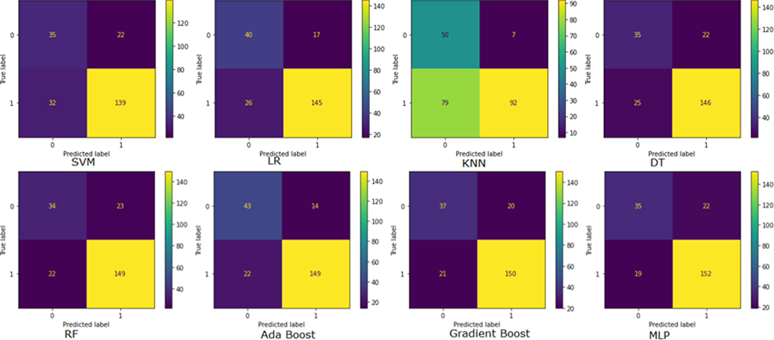
Figure 3 illustrates the confusion matrix of Supervised ML models. A confusion matrix is used to assess the model’s performance metrics. It also shows the confusion matrix of models. In this figure predicted values are shown in horizontal lines and true values are shown in vertical lines. The confusion matrix in the top right corner is derived from SVM, followed by clockwise LR, KNN, and DT on the first line. RF, AdaBoost, Gradient Boost, and MLP model confusion matrix are shown in the second row from the left. A total number of correctly classified patients when the actual value is also positive is true positive (TP). MLP has the highest TP value of 152, Gradient Boost has 150, and RF and AdaBoost both have 149. SVM, LR, and DT have TP of 139, 145, and 146, respectively. The KNN model indicates that 92 TP is the minimum. True negative (TN) is correctly classified when the actual class is negative. Three models SVM, DT, and MLP imply a 35 TN value. The rest models KNN, AdaBoost, Gradient Boost, LR, and RF represent 50, 43, 37, 40, and 34 TN values. False positives (FP) refer to misclassified patients. The MLP, DT, and SVM all show 22 FP. KNN has the lowest FP, AdaBoost, LR, Gradient Boost and RF indicate 7,14,17, 20, and 23 FP, respectively. A false negative (FN) occurs when the actual value is positive, but the prediction is negative. The highest is 79 FN by the KNN model. Models SVM, LR, and DT implied 32, 26, and 25 FN, respectively. RF and AdaBoost reported the same FN 22, while Gradient Boost reported FN 21. Based on the graph the MLP model indicated the lowest 19 FN.
Fig. 3
Confusion Matrix representation. SVM, Support vector machine classifier; LR, Logistic Regression classifier; KNN, K-Nearest Neighbors Classifier; DT, Decision Tree Classifier; RF, Random Forest Classifier; MLP, Multi-Layer Perception Classifier.
Supervised models accuracy report
The classifier train, validation, and test score are presented in Table 4. The models were trained on the training data set. The trained models were validated with 10-fold cross-validation. In this table, we represent the mean value of the validation score. After the validation process, the model is tested on the test data set. The AdaBoost model outperformed others with an 84.21% test accuracy score. Both the MLP and Gradient Boost accuracy scores are 82%. The lowest test accuracy achieved by the KNN model was 62.28%.
Table 4
Supervised models Accuracy Table
| Classifier Name | Train | Validation | Test |
| Accuracy % | score (mean) % | Accuracy % | |
| Support vector machine (SVM) | 100.00 | 90.00 | 76.32 |
| Logistic Regression (LR) | 100.00 | 91.00 | 81.14 |
| K-Nearest Neighbors (KNN) | 90.45 | 81.00 | 62.28 |
| Decision Tree (DT) | 100.00 | 84.00 | 79.39 |
| Random Forest (RF) | 100.00 | 91.00 | 80.26 |
| AdaBoost | 100.00 | 91.00 | 84.21 |
| Gradient Boost | 100.00 | 91.00 | 82.01 |
| Multi-Layer Perception (MLP) | 99.75 | 93.00 | 82.02 |
Supervised models classification report
The precision, Sensitivity, and F1-Score were used to generate the classification report. Table 5 showed the model’s detailed performance report. KNN models have the best precision score of 0.93 compared to other models, but an exceptionally low Sensitivity of 0.54 and F1-score of 0.68. Gradient Boost and RF model have remarkably similar score. Their precision, Sensitivity, and F1-score are 0.88 and 0.87 respectively. The SVM model has the lowest precision score of 0.86 among other models with 0.81 Sensitivity and 0.84 F1-score. The AdaBoost model has the second-best precision score of 0.91 and the best F1-score of 0.89, its Sensitivity score is 0.87. MLP and DT precision scores are the same 0.87. The Sensitivity score of the MLP model is 0.89 which is higher than other models with a 0.88 F1-score. DT Sensitivity and F1-score are 0.85 and 0.86. The precision, Sensitivity, and F1-score of LR model are 0.90, 0.85, and 0.87.
Table 5
Supervised Models Classification Report
| Classifier Name | Precision | Sensitivity | F1-Score |
| Support vector machine (SVM) | 0.86 | 0.81 | 0.84 |
| Logistic Regression (LR) | 0.90 | 0.85 | 0.87 |
| K-Nearest Neighbors (KNN) | 0.93 | 0.54 | 0.68 |
| Decision Tree (DT) | 0.87 | 0.85 | 0.86 |
| Random Forest (RF) | 0.87 | 0.87 | 0.87 |
| AdaBoost | 0.91 | 0.87 | 0.89 |
| Gradient Boost | 0.88 | 0.88 | 0.88 |
| Multi-Layer Perception (MLP) | 0.87 | 0.89 | 0.88 |
Supervised models AUC-ROC curve
The AUC-ROC curve is one of the most widely used evaluation metrics for classifying models. Receiver operating characteristic curves (ROCs) are used to visualize the performance of classification models. An area under the curve (AUC) represents the area beneath the entire ROC curve. False positive rates (FPR) and true positive rates (TPR) are plotted on the ROC curve. FPR on the x-axis and TPR on the y-axis. As shown in Fig. 4, the AUC-ROC curve measures the model’s AUC score.
Fig. 4
Area Under the Curve (AUC)- Receiver Operating Characteristic (ROC) Curve.
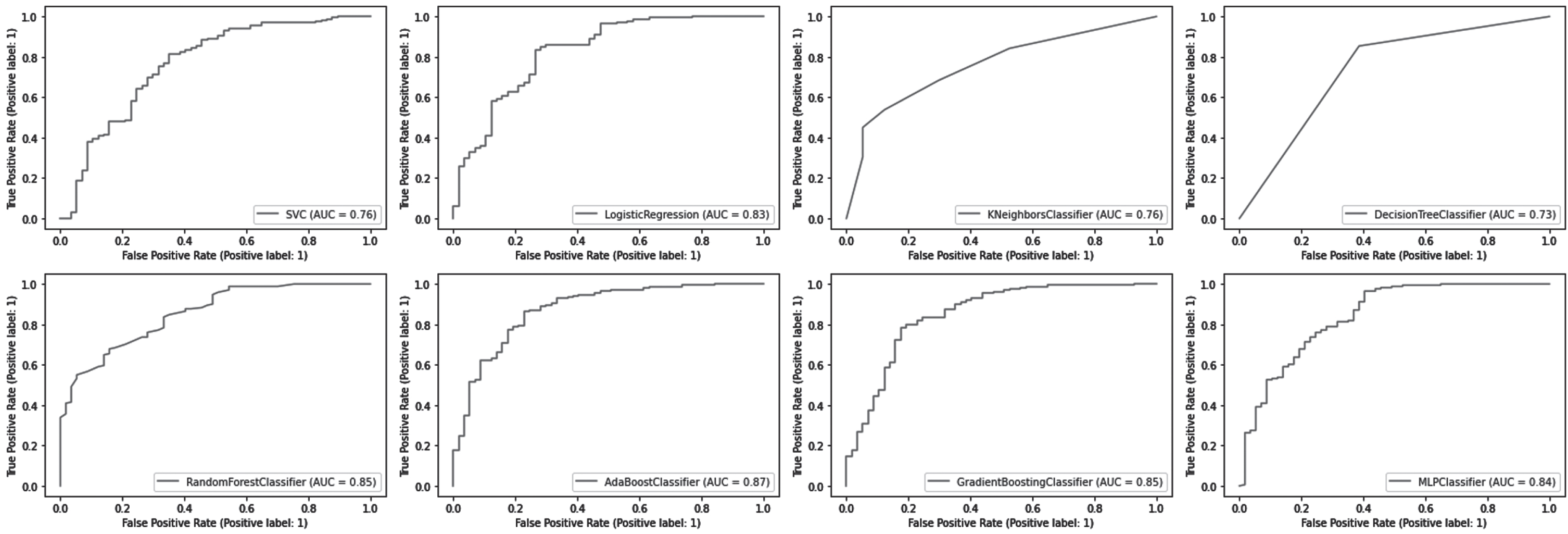
The AdaBoost classifier outperformed other models with an AUC score of 0.87. AUC scores for RF and Gradient Boost classifiers were both 0.85. For the MLP and LR models, AUC scores were 0.84 and 0.83, respectively. KNN and SVM models both have an AUC score of 0.76. The AUC score of 0.73 of the DT models is the lowest among them.
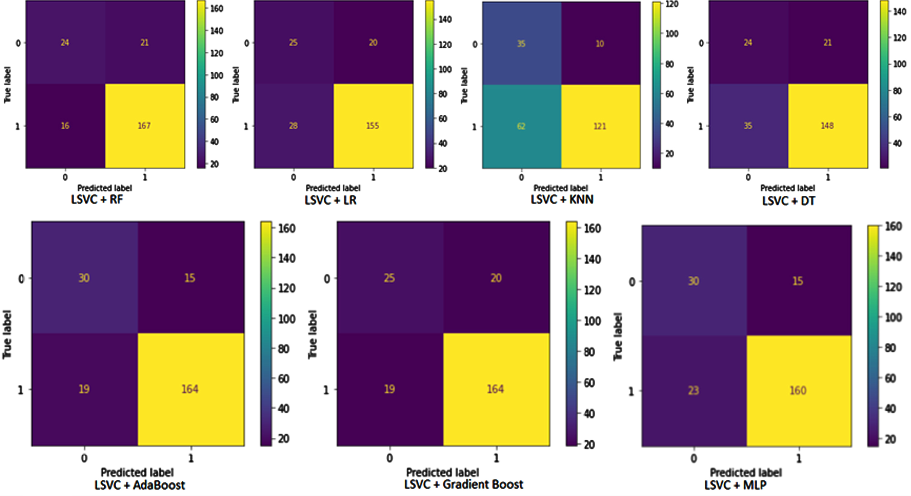
Pipelines confusion matrix
This section discusses the performance of the pipeline developed for this study. A confusion matrix of pipelines is illustrated in Fig. 5. The predicted value is shown horizontally and the actual value vertically. The first diagram illustrates the pipeline developed by combining LinearSVC and RF. In this case, TP = 167, TN = 24, FP = 21 and FN = 16. The pipelines constructed using LSVC and LR have TP = 155, TN = 25, FP = 20, and FN = 18. According to LSVC and KNN pipelines, TP is 121, TN is 35, FP is 10 and FN is 62. The DT classifier combined with LSVC resulted in TP = 148, TN = 24, FP = 21 and FN = 35 in the confusion matrix table. In the second line, the confusion matrix table is obtained from the pipeline built by AdaBoost and LSVC. According to this pipeline, there was TP = 164, FP = 15, TN = 30, and FN = 19. Based on the results of the LSVC and gradient Boost pipeline, TP = 164, FP = 20, TN = 25 and FN = 19 are shown in the confusion matrix table. A final pipeline is built using LSVC for the selection of features and MLP for the classification of patients. According to the confusion matrix table, TP = 160, FP = 15, TN = 30, and FN = 23.
Fig. 5
Pipelines confusion matrix. LSVC, Linear Support vector classifier; LR, Logistic Regression classifier; KNN, K-Nearest Neighbors Classifier; DT, Decision Tree Classifier; RF, Random Forest Classifier; MLP, Multi-Layer Perception Classifier.
Pipelines accuracy
To evaluate the performance of the pipeline, the values of TP, TN, FP, and TN are taken from the confusion matrix table. The accuracy table and classification report table provide information regarding pipeline evaluation metrics. The first column of the accuracy Table 6 values indicates the name of the model usindicate design pipeline. The accuracy of pipeline trains is shown in the second column. To validate each of the pipelines, a 10-fold validation method is used. In the validation score column, the values represent the mean value of a 10-fold validation. A pipeline test accuracy value is displayed in the accuracy column. LSVC and Ada Boost pipelines achieve the highest test accuracy of 85.09%. An 83.33% accuracy was recorded for the LSVC+MLP pipeline. A pipeline based on LSVC and KNN has the lowest accuracy of 68.42%. The test accuracy of the pipeline developed by LSVC and RF, LR, DT, and Gradient Boost is 83.77, 78.95, 75.44, and 82.89, respectively.
Table 6
Pipelines Accuracy Table
| Pipeline Name | Train Accuracy % | Validation score (mean) % | Test Accuracy % |
| Linear support vector classifier (LSVC) and Random Forest (RF) | 100.00 | 91.00 | 83.77 |
| Linear support vector classifier (LSVC) and Logistic Regression (LR) | 100.00 | 90.00 | 78.95 |
| Linear support vector classifier (LSVC) and K-Nearest Neighbors (KNN) | 83.73 | 76.00 | 68.42 |
| Linear support vector classifier (LSVC) and Decision Tree (DT) | 100.00 | 84.00 | 75.44 |
| Linear support vector classifier (LSVC) and AdaBoost | 100.00 | 89.00 | 85.09 |
| Linear support vector classifier (LSVC) and Gradient Boost | 100.00 | 88.00 | 82.89 |
| Linear support vector classifier (LSVC) and Multi-Layer Perception | 99.74 | 91.00 | 83.33 |
Pipeline classification report
A pipeline classification report Table 7 displays precision, Sensitivity, and F1-score values. The pipeline name is included in the column titled “Pipeline”. Each pipeline’s precision, Sensitivity, and F1-score values are represented by columns and rows.
Table 7
Pipelines Classification Report Table
| Pipeline Name | Precision | Sensitivity | F1-Score |
| Linear support vector classifier (LSVC) and Random Forest (RF) | 0.89 | 0.91 | 0.90 |
| Linear support vector classifier (LSVC) and Logistic Regression (LR) | 0.89 | 0.85 | 0.87 |
| Linear support vector classifier (LSVC) and K-Nearest Neighbors (KNN) | 0.92 | 0.66 | 0.77 |
| Linear support vector classifier (LSVC) and Decision Tree (DT) | 0.88 | 0.81 | 0.84 |
| Linear support vector classifier (LSVC) and AdaBoost | 0.92 | 0.90 | 0.91 |
| Linear support vector classifier (LSVC) and Gradient Boost | 0.89 | 0.90 | 0.89 |
| Linear support vector classifier (LSVC) and Multi-Layer Perception | 0.91 | 0.87 | 0.89 |
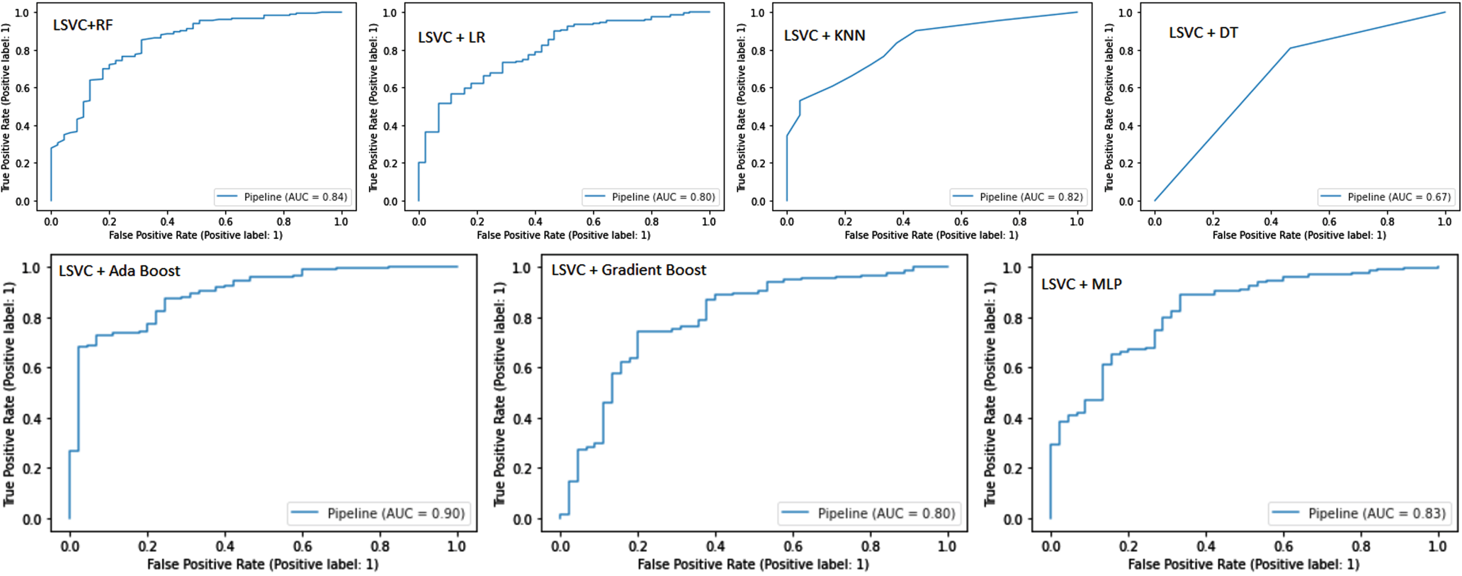
Pipeline ROC-AUC curve
Figure 6 shows the ROC-AUC curve for pipelines. LSVC and Ada Boost achieved the best AUC score of 0.90. LSVC and RF achieved an AUC score of 0.84. The MLP pipeline achieved an AUC score of 0.83. The LR and Gradient Boost pipelines developed from LSVC selected features achieved an AUC score of 0.80. The KNN and DT pipelines achieved AUC scores of 0.82 and 0.67, respectively.
Comparison of supervised models and pipelines
As described in the previous section, traditional machine learning models and pipelines can be compared. A comparison of train validation and test accuracy scores for models and pipelines is presented in Tables 4 and 6. A total of 756 input features were used in this study. Table 4 summarizes the performance of the models with all the input features based on the feature selection technique from model LSVC, whereas Table 6 shows the performance of the pipeline after it has been reduced to only the most relevant features of the input. In this study, we construct seven pipelines with the same classifier used in the previous part. In most cases, the classifier performance is significantly improved based on the test accuracy score. The RF classifier test accuracy was 80.26 whereas the pipeline combination of LSVC features selection and RF classification accuracy significantly improved to 83.77. The pipeline with KNN accuracy increased from 62.28 to 68.48. Ada Boost pipeline test accuracy increased to 85.09 from 84.21. Gradient Boost pipeline accuracy grew up to 82.89 from 82.01. The accuracy of the pipeline created with MLP is boosted to 83.33 from 82.01. Two pipelines’ performance does not improve compared to their previous accuracy score. The pipelines of LR and DT accuracy dropped from 81.14 and 79.39 to 78.95 and 75.44, respectively.
The precision, sensitivity, and F1-score of ML models and pipelines were exemplified in Tables 5 and 7. Based on the values summarized in these tables, we can conclude that the pipelines outperformed the traditional ML models. The pipelines created by selecting features from the model and using a conventional classifier achieved better precision, Sensitivity, and F1-score. The AUC score from the ROC-AUC curve significantly improved because of the pipelines.
DISCUSSION
The present work has reviewed and compared the most relevant studies on PD classification by consulting reliable literature repositories. The methodology for PD classification and the challenges involved in each study were considered. Most of the research published was focused on identifying the factors that cause disease to diagnose or monitor it.
Using diffusion tensor imaging (DTI), an ensemble learning framework based on two layers of stacking was developed. This study has evaluated four traditional classifiers: support vector machines (SVM), K-nearest neighbors (KNN), random forests (RF), and artificial neural networks (ANN). At the second layer, a logistic regression classifier (LR) is used to classify PD [35]. Another work has used electroencephalography (EEG) data to classify PD with SVM and K-NN classifiers. Patients with PD commonly experience cognitive symptoms. To classify PD patients, they analyze EEG features collected from daily clinical activities [36]. Both studies included medical images and collected data from fewer than 120 individuals. In contrast, our chosen data set contained voice records from PD patients and healthy controls with more instances and attributes.
The goal of another work was to determine which deep brain stimulation (DBS) parameters are optimal for PD using functional magnetic resonance imaging (fMRI) and ML. Their model predicts optimal and non-optimal DBS settings based on fMRI patterns collected from patients with PD [37]. Another investigation examined the DBS parameters of PD patients over three to twelve months. The data were recorded and analyzed using SVM to diagnose the patients. These results suggest that ML models can accurately predict levodopa states based on personally classified engineered features [38].
A Naive Bayes ML model with feature selection was developed by another study. The team uses Fisher score feature selection, correlated feature selection, and mutual information-based feature selection strategies to create the collaborative feature bank. The Naïve Bayes model achieved good results when it was combined with the collaborative feature [39]. As part of this work, voice data from PD patients were analyzed using naive Bayes algorithms. The present study has used other supervised algorithms to select the best algorithms to analyze high-dimensional data.
It has been hypothesized that relevant lipidomics can predict PD severity. ML model was used to analyze blood samples from PD patients to identify lipid signatures predicting motor severity [40]. A ML approach was used to identify lipid signatures which capable of predicting motor severity in PD. Another analysis was centered on voice record data. PD patients were categorized using classification and regression trees (CART), support vector machines (SVM), and artificial neural networks (ANN). Participants included 31 subjects and 195 records (23 PD and 8 control) [41].
A novel web-based approach was proposed to detect Parkinsonians from web search engine users (Google, Bing). Based on mouse and keyboard interaction with a search engine, supervised ML classifiers are capable of showing the faster progression of Parkinson’s-related signs in individuals who have screened positive [42]. To identify the best combinations of clinical features to predict motor outcome (MDS-UPDRS-III) in PD, another investigation has evaluated 204 PD patients with 18 clinical features in multiple randomized arrangements. With automated hyperparameter tuning and optimal use of FSSAs and predictor algorithms, it was demonstrated excellent prediction of motor outcomes in PD patients [43].
In the advanced stages of PD, more than half of the patient’s experience freezing of gait (FOG). The methodology involved segmenting the angular velocity signals and subsequently extracting features in both the time and frequency domains. FOG and pre-FOG episodes were detected using several machine learning classifiers [44]. Policy iteration of Markov decision processes (MDP) was used to analyze clinically relevant disease states and to determine optimal medication combinations. They examined combinations of PD medications as well as motor symptom severity. After following PD patients for 55.5 months, reinforcement learning (RL) was used to develop a sequential decision-making rule to minimize motor symptoms. A machine-physician system based on evidence-based medicine may help improve PD management through this study [45].
The present study has developed a model of early PD progression incorporating intra-individual variability and medication effects was also developed. This study supports nondeterministic models and suggests that static subtype designations may not fully capture the PD spectrum. Four hundred and twenty-three patients with early PD and 196 healthy controls were studied for up to seven years. The disease states are defined using contrastive latent variables followed by hidden Markov models. An analysis of seven key motor or cognitive outcomes not included in the learning phase was conducted [46].
Several investigations have used ML models to classify PD. A well-trained model would be able to diagnose PD accurately and support clinical systems. In the above discussion we have analyzed different methods to classify. In these studies, different types of data have been analyzed and conclusions have been drawn. These studies did not mention a methodology for diagnosing PD patients based on high-dimensional daily activity data. In the present work supervised ML models and pipelines were developed, trained, and evaluated their performance on high dimensional data set.
The primary limitation of this study restricts the dataset itself, which lacks comprehensive information regarding the disease stage, treatment, and duration for the included patients. This limitation is attributable to the utilization of openly accessible data. Since we solely relied on publicly available data and were not involved in the data collection process, we are unable to directly mitigate this constraint. Regrettably, we are unable to address this limitation without the cooperation of the data owner.
Conclusions
This study has evaluated several supervised machine learning classifiers and multilayer classifiers (MLP). Model performance was evaluated using evaluation metrics. AdaBoost classifiers were the most accurate at 84.21%, while KNN classifiers were the least accurate at 62.28%. The AdaBoost algorithms also achieved the highest precision and F1-scores of 0.91 and 0.89, respectively. The highest sensitivity or sensitivity score was obtained by MLP, which was 0.89.
Pipelines were designed using ML classifiers and MLP. Almost all algorithm accuracy scores improved after implementing the pipeline, except for LR. The best pipeline for accuracy was AdaBoost with LSVC, which had 85.09% accuracy, which is significantly higher than AdaBoost alone. In addition, the F1-score, precision, and sensitivity of the AdaBoost pipeline improved significantly from 0.89 to 0.91, 0.91 to 0.92, and 0.87 to 0.90, respectively. These improvements were also observed for other pipelines as well. In terms of accuracy, precision, Sensitivity, and F1-score, the improved pipeline classifiers outperformed the supervised machine learning classifiers.
Based on speech biomarkers, ML classifiers and pipelines have been demonstrated to be capable of classifying PD patients. The pipelines were more effective at selecting the most relevant features of high-dimensional data and at classifying PD more accurately.
The current treatments for PD offer only temporary relief of motor symptoms through improving the dopamine deficit or through surgical procedures. To diagnose neurodegenerative disorders more accurately, and to identify populations at risk for neuroprotective treatment, further research on specific/differential biomarkers is required. The proposed approach may represent a starting point for the detection of early forms of PD.
ACKNOWLEDGMENTS
We are grateful to the staff of the Telemedicine and Telepharmacy Center of the University of Camerino for helpful suggestions and discussion.
FUNDING
This work was supported by an institutional grant of the University of Camerino.
CONFLICTS OF INTEREST
The authors have no conflict of interest to report.
DATA AVAILABILITY
The dataset used in this study are available upon reasonable request from the corresponding author.
REFERENCES
[1] | Chin-Chan M , Navarro-Yepes J , Quintanilla-Vega B ((2015) ) Environmental pollutants as risk factors for neurodegenerative disorders: Alzheimer and Parkinson diseases. Front Cell Neurosci 9: , 124. |
[2] | Hamza TH , Chen H , Hill-Burns EM , Rhodes SL , Montimurro J , Kay DM , Tenesa A , Kusel VI , Sheehan P , Eaaswarkhanth M , Yearout D , Samii A , Roberts JW , Agarwal P , Bordelon Y , Park Y , Wang L , Gao J , Vance JM , Kendler KS , Bacanu S-A , Scott WK , Ritz B , Nutt J , Factor SA , Zabetian CP , Payami H ((2011) ) Genome-wide gene-environment study identifies glutamate receptor gene GRIN2A as a Parkinson’s disease modifier gene via interaction with coffee. PLOS Genet 7: , e1002237. |
[3] | Tysnes O-B , Storstein A ((2017) ) Epidemiology of Parkinson’s disease. J Neural Transm 124: , 901–905. |
[4] | Noyce AJ , Rees RN , Acharya AP , Schrag A ((2018) ) An early diagnosis is not the same as a timely diagnosis of Parkinson’s disease. F1000Res 7: , F1000 Faculty Rev-1106. |
[5] | Ray Dorsey E , Elbaz A , Nichols E , Abd-Allah F , Abdelalim A , Adsuar JC , Ansha MG , Brayne C , Choi JYJ , Collado-Mateo D , Dahodwala N , Do HP , Edessa D , Endres M , Fereshtehnejad SM , Foreman KJ , Gankpe FG , Gupta R , Hankey GJ , Hay SI , Hegazy MI , Hibstu DT , Kasaeian A , Khader Y , Khalil I , Khang YH , Kim YJ , Kokubo Y , Logroscino G , Massano J , Ibrahim NM , Mohammed MA , Mohammadi A , Moradi-Lakeh M , Naghavi M , Nguyen BT , Nirayo YL , Ogbo FA , Owolabi MO , Pereira DM , Postma MJ , Qorbani M , Rahman MA , Roba KT , Safari H , Safiri S , Satpathy M , Sawhney M , Shafieesabet A , Shiferaw MS , Smith M , Szoeke CEI , Tabarés-Seisdedos R , Truong NT , Ukwaja KN , Venketasubramanian N , Villafaina S , Weldegwergs KG , Westerman R , Wijeratne T , Winkler AS , Xuan BT , Yonemoto N , Feigin VL , Vos T , Murray CJL ((2018) ) Global, regional, and national burden of Parkinson’s disease, 1990–2016: A systematic analysis for the Global Burden of Disease Study 2016. Lancet Neurol 17: , 939–953. |
[6] | Jankovic J ((2008) ) Parkinson’s disease: Clinical features and diagnosis. J Neurol Neurosurg Psychiatry 79: , 368 LP–376. |
[7] | Tolosa E , Garrido A , Scholz SW , Poewe W ((2021) ) Challenges in the diagnosis of Parkinson’s disease. Lancet Neurol 20: , 385–397. |
[8] | Ho AK , Iansek R , Marigliani C , Bradshaw JL , Gates S ((1999) ) Speech impairment in a large sample of patients with Parkinson’s disease. Behav Neurol 11: , 131–137. |
[9] | Sapir S , Ramig LO , Hoyt P , Countryman S , O’Brien C , Hoehn M ((2002) ) Speech loudness and quality 12 months after intensive voice treatment (LSVT) for Parkinson’s disease: A comparison with an alternative speech treatment. Folia Phoniatr Logop 54: , 296–303. |
[10] | Baker KK , Ramig LO , Luschei ES , Smith ME ((1998) ) Thyroarytenoid muscle activity associated with hypophonia in Parkinson disease and aging. Neurology 51: , 1592–1598. |
[11] | Trail M , Fox C , Olson L , Sapir S , Howard J ((2005) ) Speech treatment for Parkinson’s disease. NeuroRehabilitation 20: , 205–221. |
[12] | Postuma RB , Berg D , Stern M , Poewe W , Olanow CW , Oertel W , Obeso J , Marek K , Litvan I , Lang AE , Halliday G , Goetz CG , Gasser T , Dubois B , Chan P , Bloem BR , Adler CH , Deuschl G ((2015) ) MDS clinical diagnostic criteria for Parkinson’s disease. Mov Disord 30: , 1591–1601. |
[13] | Postuma RB , Poewe W , Litvan I , Lewis S , Lang AE , Halliday G , Goetz CG , Chan P , Slow E , Seppi K , Schaffer E , Rios-Romenets S , Mi T , Maetzler C , Li Y , Heim B , Bledsoe IO , Berg D ((2018) ) Validation of the MDS clinical diagnostic criteria for Parkinson’s disease. Mov Disord 33: , 1601–1608. |
[14] | Heinzel S , Berg D , Gasser T , Chen H , Yao C , Postuma RB ((2019) ) Update of the MDS research criteria for prodromal Parkinson’s disease. Mov Disord 34: , 1464–1470. |
[15] | Meigal AI , Rissanen S , Tarvainen MP , Karjalainen PA , Iudina-Vassel IA , Airaksinen O , Kankaanpää M ((2009) ) Novel parameters of surface EMG in patients with Parkinson’s disease and healthy young and old controls. J Electromyogr Kinesiol 19: , e206–13. |
[16] | Lowit A , Dobinson C , Timmins C , Howell P , Kröger B ((2010) ) The effectiveness of traditional methods and altered auditory feedback in improving speech rate and intelligibility in speakers with Parkinson’s disease. Int J Speech Lang Pathol 12: , 426–436. |
[17] | Kumar NS , Selvi MS , Gayathri D ((2021) ) A multiple feature selection based Parkinson’s disease diagnostic system using deep learning neural network classifier. NeuroQuantology 19: , 209–220. |
[18] | Mei J , Desrosiers C , Frasnelli J ((2021) ) Machine learning for the diagnosis of Parkinson’s disease: A review of literature. Front Aging Neurosci 13: , 633752. |
[19] | Chen M , Hao Y , Hwang K , Wang L , Wang L ((2017) ) Disease prediction by machine learning over big data from healthcare communities. IEEE Access 5: , 8869–8879. |
[20] | Archenaa J , Anita EAM ((2015) ) A survey of big data analytics in healthcare and government. Procedia Comput Sci 50: , 408–413. |
[21] | Haq AU , Li JP , Memon MH , khan J , Malik A , Ahmad T , Ali A , Nazir S , Ahad I , Shahid M ((2019) ) Feature selection based on L1-norm support vector machine and effective recognition system for Parkinson’s disease using voice recordings. IEEE Access 7: , 37718–37734. |
[22] | Erdogdu Sakar B , Serbes G , Sakar CO ((2017) ) Analyzing the effectiveness of vocal features in early telediagnosis of Parkinson’s disease. PLoS One 12: , e0182428. |
[23] | Peker M , Sen B , Delen D ((2015) ) Computer-aided diagnosis of Parkinson’s disease using complex-valued neural networks and mRMR feature selection algorithm. J Healthc Eng 6: , 281–302. |
[24] | Peker M ((2016) ) A decision support system to improve medical diagnosis using a combination of k-medoids clustering based attribute weighting and SVM. J Med Syst 40: , 116. |
[25] | Zhu X , Davidson I (2007) Knowledge Discovery and Data Mining: Challenges and Realities: Challenges and Realities, Igi Global. |
[26] | Sakar CO , Serbes G , Gunduz A , Tunc HC , Nizam H , Sakar BE , Tutuncu M , Aydin T , Isenkul ME , Apaydin H ((2019) ) A comparative analysis of speech signal processing algorithms for Parkinson’s disease classification and the use of the tunable Q-factor wavelet transform. Appl Soft Comput J 74: , 255–263. |
[27] | Sakar C , Serbes G , Gunduz A , Nizam H , Sakar B (2018) Parkinson’s Disease classification. UCI Machine Learning Repository. https://doi.org/10.24432/C5MS4X. |
[28] | Tunc HC , Sakar CO , Apaydin H , Serbes G , Gunduz A , Tutuncu M , Gurgen F ((2020) ) Estimation of Parkinson’s disease severity using speech features and extreme gradient boosting. Med Biol Eng Comput 58: , 2757–2773. |
[29] | Tsanas A , Little MA , McSharry PE , Spielman J , Ramig LO ((2012) ) Novel speech signal processing algorithms for high-accuracy classification of Parkinsons disease. IEEE Trans Biomed Eng 59: , 1264–1271. |
[30] | Little MA , McSharry PE , Hunter EJ , Spielman J , Ramig LO ((2009) ) Suitability of dysphonia measurements for telemonitoring of Parkinson’s disease. IEEE Trans Biomed Eng 56: , 1015–1022. |
[31] | Bowyer KW , Chawla NV , Hall LO , Kegelmeyer WP ((2011) ) {SMOTE:} Synthetic Minority Over-sampling Technique. CoRR abs/1106.1: . |
[32] | Pedregosa F , Varoquaux G , Gramfort A , Michel V , Thirion B , Grisel O , Blondel M , Prettenhofer P , Weiss R , Dubourg V , Vanderplas J , Passos A , Cournapeau D , Brucher M , Perrot M , Duche E ((2011) ) Scikit-learn: Machine Learning in Python. J Mach Learn Res 12: , 2825–2830. |
[33] | Tolles J , Meurer WJ ((2016) ) Logistic regression: Relating patient characteristics to outcomes. JAMA 316: , 533–534. |
[34] | Akanbi OA , Amiri IS , Fazeldehkordi E (2015) Chapter 3 - Research Methodology. In A Machine-Learning Approach to Phishing Detection and Defense, Akanbi OA, Amiri IS, Fazeldehkordi E, eds. Syngress, Boston, pp. 35–43. |
[35] | Yang Y , Wei L , Hu Y , Wu Y , Hu L , Nie S ((2021) ) Classification of Parkinson’s disease based on multi-modal features and stacking ensemble learning. J Neurosci Methods 350: , 109019. |
[36] | Betrouni N , Delval A , Chaton L , Defebvre L , Duits A , Moonen A , Leentjens AFG , Dujardin K ((2019) ) Electroencephalography-based machine learning for cognitive profiling in Parkinson’s disease: Preliminary results. Mov Disord 34: , 210–217. |
[37] | Boutet A , Madhavan R , Elias GJB , Joel SE , Gramer R , Ranjan M , Paramanandam V , Xu D , Germann J , Loh A , Kalia SK , Hodaie M , Li B , Prasad S , Coblentz A , Munhoz RP , Ashe J , Kucharczyk W , Fasano A , Lozano AM ((2021) ) Predicting optimal deep brain stimulation parameters for Parkinson’s disease using functional MRI and machine learning. Nat Commun 12: , 3043. |
[38] | Sand D , Rappel P , Marmor O , Bick AS , Arkadir D , Lu BL , Bergman H , Israel Z , Eitan R ((2021) ) Machine learning-based personalized subthalamic biomarkers predict ON-OFF levodopa states in Parkinson patients. J Neural Eng 18: , doi: 10.1088/1741-2552/abfc1d. |
[39] | Pramanik M , Pradhan R , Nandy P , Qaisar SM , Bhoi AK ((2021) ) Assessment of acoustic features and machine learning for Parkinson’s detection. J Healthc Eng 2021: , 9957132. |
[40] | Avisar H , Guardia-Laguarta C , Area-Gomez E , Surface M , Chan AK , Alcalay RN , Lerner B ((2021) ) Lipidomics prediction of Parkinson’s disease severity: A machine-learning analysis. J Parkinsons Dis 11: , 1141–1155. |
[41] | Karapinar Senturk Z ((2020) ) Early diagnosis of Parkinson’s disease using machine learning algorithms. Med Hypotheses 138: , 109603. |
[42] | Youngmann B , Allerhand L , Paltiel O , Yom-Tov E , Arkadir D ((2019) ) A machine learning algorithm successfully screens for Parkinson’s in web users. Ann Clin Transl Neurol 6: , 2503–2509. |
[43] | Salmanpour MR , Shamsaei M , Saberi A , Klyuzhin IS , Tang J , Sossi V , Rahmim A ((2020) ) Machine learning methods for optimal prediction of motor outcome in Parkinson’s disease. Phys Medica 69: , 233–240. |
[44] | Borzì L , Mazzetta I , Zampogna A , Suppa A , Olmo G , Irrera F ((2021) ) Prediction of freezing of gait in parkinson’s disease usingwearables and machine learning.. Sensors (Switzerland) 21: , 614. |
[45] | Kim Y , Suescun J , Schiess MC , Jiang X ((2021) ) Computational medication regimen for Parkinson’s disease using reinforcement learning. Sci Rep 11: , 9313. |
[46] | Severson KA , Chahine LM , Smolensky LA , Dhuliawala M , Frasier M , Ng K , Ghosh S , Hu J ((2021) ) Discovery of Parkinson’s disease states and disease progression modelling: A longitudinal data study using machine learning. Lancet Digit Heal 3: , e555–e564. |

