


Abstract
The Galactic interstellar medium abounds in shocks with low velocities vs ≲ 70 km s−1. Some are descendants of higher velocity shocks, while others start off at low velocity (e.g., stellar bow shocks, intermediate velocity clouds, spiral density waves). Low-velocity shocks cool primarily via Lyα and two-photon continuum, augmented by optical recombination lines (e.g., Hα), forbidden lines of metals and free-bound emission, free–free emission. The dark far-ultraviolet (FUV) sky, aided by the fact that the two-photon continuum peaks at 1400 Å, makes the FUV band an ideal tracer of low-velocity shocks. GALEX FUV images reaffirm this expectation, discovering faint and large interstellar structure in old supernova remnants and thin arcs stretching across the sky. Interstellar bow shocks are expected from fast stars from the Galactic disk passing through the numerous gas clouds in the local interstellar medium within 15 pc of the Sun. Using the bests atomic data available to date, we present convenient fitting formulae for yields of Lyα, two-photon continuum, and Hα for pure hydrogen plasma in the temperature range of 104–105 K. The formulae presented here can be readily incorporated into time-dependent cooling models as well as collisional ionization equilibrium models.
Export citation and abstract BibTeX RIS

Original content from this work may be used under the terms of the Creative Commons Attribution 3.0 licence. Any further distribution of this work must maintain attribution to the author(s) and the title of the work, journal citation and DOI.
1. Motivation
Supernova remnants and stellar wind bubbles are iconic examples of shocks in the interstellar medium (ISM). These shocks, with the passage of time, descend to lower velocities. Our interest here is shocks with velocities less than 70 km s−1. The post-shock temperature depends on the mean molecular mass, but we adopt a fiducial value of Ts ≲ 105 K and investigate the cooling of such shock-heated hydrogen gas. These shocks cool primarily via Lyα (whose photons are trapped within the shocked region and eventually die on a dust particle) and two-photon continuum. The latter can be detected by Far Ultra-Violet (FUV) imagers. Low-velocity shocks also arise on Galactic length scales: intermediate-velocity and high-velocity clouds raining down from the lower halo into the disk and gas that is shocked as it enters a spiral arm. Vallée (2017) provides a good description of the Milky Way's spiral arms, and Kim et al. (2008) discuss Galactic interstellar shocks.pre
Stellar bow shocks are another major source of low-velocity shocks. For instance, consider our own Sun, a generic G5V star with a weak stellar wind (2 × 10⁻¹⁴ M⊙ yr−1 ) moving into a warm (∼7000 K) and partially ionized cloud (ionization fraction, x ≈ 1/3 ) at a relative speed of 23–26 km s−1 (Frisch et al. 2011; McComas et al. 2012; Zank et al. 2013; Gry & Jenkins 2014). Because this velocity may not be larger than the fast-mode magnetosonic velocity of the interstellar cloud, there may be a "bow wave" instead of a bow shock (McComas et al. 2012). In the Galactic disk, interstellar space is occupied by the Warm Neutral Medium (WNM; 103–8 × 10³ K), the Warm Ionized Medium (WIM; 8 × 10³ K), and the Hot Ionized Medium (HIM; 105–106 K), in roughly equal proportions.
From studies with SDSS-Apogee and Gaia-DR2 (Anguiano et al. 2020), the 3D velocity dispersion of the typical (α-abundance tagged) thin-disk star is 48 km s−1, whereas those belonging to the thick disk have dispersion of 87 km s−1. The majority of these local stars reside in the thin disk with a density ratio nthin/nthick = 2.1 ± 0.2. As discussed in a previous study (Shull & Kulkarni 2023), a sizable number of stars should be moving supersonically through ambient gas in the WNM and WIM. 4 The sizes of the resulting bow shocks will be determined by the stellar velocity and the magnitude of the stellar wind.
Separately, recent developments warrant a closer look at low-velocity shocks. We draw attention to the discoveries of three large-diameter supernova remnants (Fesen et al. 2021) and a 30° long, thin arc in Ursa Major (Bracco et al. 2020). In large part, these findings were made possible with a new diagnostic—GALEX FUV continuum imaging. The detection of such faint, extended features demonstrates simultaneously the value of the dark FUV sky (O'Connell 1987) as well as the value of the FUV band in detecting two-photon emission, a distinct diagnostic of warm (T ≲ 105 K) shocked gas (Bracco et al. 2020; Kulkarni 2022).
The principal goal of this paper is to develop accurate hydrogen plasma cooling models, paying attention to the production of the two-photon continuum in warm plasma, T ≲ 105 K, the temperature range of interest to low velocity shocks. To this end, we first derive the probability of Lyα, two-photon continuum, and Hα emission resulting from excitation of the ground state of hydrogen to all n ℓ levels for n ≤ 5 (Section 2). Next, we review rate coefficients for line excitation by collisions with electrons (Section 3), followed by a review of collisional ionization (Section 4). The results are combined to construct a cooling curve for warm hydrogen plasma (Section 5). In Section 6 we present a comprehensive (isobaric and isochoric) cooling framework. In Section 7 we apply this model to representative low-velocity shocks and then compute the cumulative photon (Lyα, 2γ and Hα) yields over a grid of post-shock temperatures and initial ionization fractions. In Section 8 we summarize our results and discuss future prospects. Unless otherwise stated, the atomic line data (A-coefficients, term values) are from the NIST Atomic Spectra Database 5 and basic formulae from Draine (2011).
2. Two-photon Production
Colliding electrons excite hydrogen atoms to various levels and, if sufficiently energetic, ionize H i to H ii. Excited levels are also populated by radiative recombination. Excited hydrogen atoms return to the ground state, some by emitting a Lyman-series photon and others via a cascade of optical/IR recombination lines and ending with Lyα emission. Atoms that find themselves in the metastable 2s2S1/2 level, if undisturbed over a timescale of  s, return to the ground state by emitting a two-photon continuum. Here, A2s→1s
= 8.23 s−1 is the Einstein A-coefficient for the 2s − 1s transition (Drake 1986). Its value should be compared to those for allowed transitions (e.g., 6.26 × 10⁸ s−1 for Lyα and (1–5) × 107 s−1 for Hα, depending on the upper levels, 3s, 3p, 3d, involved).
s, return to the ground state by emitting a two-photon continuum. Here, A2s→1s
= 8.23 s−1 is the Einstein A-coefficient for the 2s − 1s transition (Drake 1986). Its value should be compared to those for allowed transitions (e.g., 6.26 × 10⁸ s−1 for Lyα and (1–5) × 107 s−1 for Hα, depending on the upper levels, 3s, 3p, 3d, involved).
The goal of this section is to compute the production of Lyα photons, two-photon continuum, and Hα resulting from electronic excitation of H atoms. We consider excitations to 14 n
ℓ levels; see Table 2 for term values and index scheme. We make the following two assumptions. (1) The proton density in the plasma is less than the "2s critical density" of 1.5 × 104 cm−3 (see Chapter 14 of Draine 2011). This ensures that atoms in the 2s level are not collisionally mixed to the 2p level over a timescale of  and thus relax by emitting a two-photon continuum. (2) The cooling plasma is optically thick to Lyman lines, so that Lyman photons are absorbed in the vicinity of where they are emitted. Thus, when computing branching ratios, all allowed Lyman series recombinations can be ignored (case B).
2.1. Photon Yields
Consider, for example, an atom excited to one of the n = 3 levels. An atom excited to 3s or 3d will decay to 2p by emitting Hα followed by Lyα. We ignore forbidden transitions such as ns − 1s two-photon decays; see Chluba & Sunyaev (2008). An atom excited to 3p can decay by emitting Lyβ or decay to 2s by emitting Hα followed by two-photon decay. For the latter, the branching fraction  for Lyβ emission is A3p→1s
/(A3p→1s
+ A3p→2s
) ≈ 88%. However, under case B, the Lyβ photon will be absorbed elsewhere in the nebula, and the situation will be repeated until de-excitation ends with emission of Hα+Lyα.
for Lyβ emission is A3p→1s
/(A3p→1s
+ A3p→2s
) ≈ 88%. However, under case B, the Lyβ photon will be absorbed elsewhere in the nebula, and the situation will be repeated until de-excitation ends with emission of Hα+Lyα.
For a fiducial value of optical depth (τ0,α
= 1000 ) of Lyα, Table 1 lists the corresponding optical depths for the Lyman series. The branching ratio  to emit a Lyγ line is slightly smaller that that for Lyβ. As with Lyβ under case-B conditions, Lyγ will also be converted to some combination of Lyα, optical/IR recombination lines, and a two-photon continuum. The Lyman series oscillator strengths, f ∝ n−3, where n is the principal quantum number of the excited state. Thus the Lyman-line optical depths decrease rapidly with increasing n (up the series). In contrast, the branching factors
  decrease slowly with n.
Table 1. Lyman Lines: Optical Depths and Scatterings
| line | λ (Å) | f | τ0 | n ℓ |

|
|---|---|---|---|---|---|
| Lyα | 1215.67 | 0.4164 | 1000 | 2p | 1 |
| Lyβ | 1025.73 | 0.07912 | 160 | 3p | 0.881 |
| Lyγ | 972.54 | 0.02901 | 56 | 4p | 0.839 |
| Lyδ | 949.74 | 0.01394 | 26 | 5p | 0.819 |
Note. Columns 1–4 give the name, wavelength, absorption oscillator strength, and central optical depth of the line. The column density of the nebula is assumed to provide a line-center optical depth of τ0 = 1000 for Lyα, from which τ0 for other Lyman lines follow.  (column 6) is the branching ratio for an atom excited to an np level (column 5) to relax by emitting the appropriate Lyman series line, as opposed to a multi-decay cascade.
Download table as: ASCIITypeset image
All states other than ns states have fine structure. For example, the 4p state has two levels, P1/2 and P3/2, with very little energy difference between the fine structure levels. The electron collisional excitation rate coefficients presented below (Section 3) refer to the sum of transitions to the entire level, e.g., 1s → 4p. The photon yields for Lyα, 2γ continuum, and Hα are given in Table 2.
Table 2. Photon Yields for Lyα, Hα, and 2γ Continuum
| k | Level | pk (Lyα) | pk (Hα) | pk (2γ) |
|---|---|---|---|---|
| 1 | 2s | 0 | 0 | 1 |
| 2 | 2p | 1 | 0 | 0 |
| 3 | 3s | 1 | 1 | 0 |
| 4 | 3p | 0 | 1 | 1 |
| 5 | 3d | 1 | 1 | 0 |
| 6 | 4s | 0.585 | 0.415 | 0.415 |
| 7 | 4p | 0.261 | 0.261 | 0.739 |
| 8 | 4d | 0.813 | 0.187 | 0.187 |
| 9 | 4f | 1 | 1 | 0 |
| 10 | 5s | 0.513 | 0.378 | 0.487 |
| 11 | 5p | 0.305 | 0.265 | 0.695 |
| 12 | 5d | 0.687 | 0.267 | 0.313 |
| 13 | 5f | 0.936 | 0.702 | 0.064 |
| 14 | 5g | 1 | 1 | 0 |
Note. Photon production yields pk of Lyα (column 3), Hα (column 4), and two-photon continuum (column 5) upon excitation from ground state (1s) to level n ℓ (column 2). The transitions are also labeled by an index k (column 1). At the precision of this work the energy level depends only on the energy wavenumber: 82,303 cm−1 (n = 2), 97,544 cm−1 (n = 3), 102,879 cm−1 (n = 4) and 105,348 cm−1 (n = 5). As a guide to interpreting this table we note that an H atom excited to k = 3 (3s) relaxes by emitting one Hα photon, one Lyα photon but no two-photon continuum.
Download table as: ASCIITypeset image
3. Electron Collisional Excitation
The excitation of lines of hydrogen due to collisions with electrons is a venerable topic in ISM studies. The classic review by Dalgarno & McCray (1972) summarized the atomic physics of the 1960s. Scholz & Walters (1991) undertook detailed calculations of the n = 1 → 2 excitations and also provided an estimate for the H I cooling rate coefficient, ΛH I. Anderson et al. (2002); see also Anderson et al. (2000) present close-coupling R-matrix calculations. We adopt these rates since they offer improved accuracy over previous studies (Scholz et al. 1990). The Anderson et al. (2002) theoretical cross sections were constructed with 15 physical energy states up to n = 5 (1s to 5g) supplemented by 24 pseudo-states described by orbitals ( ) with
  and
and  .
.
Anderson et al. (2002) present collision strengths,  , for excitation from levels i to j (see Figure 1), averaged over a Maxwellian velocity distribution at electron energies, ET
≡ kB
T, ranging from 0.5 to 25 eV. The collisional excitation rate coefficients (in cm3 s−1) are then given by:
, for excitation from levels i to j (see Figure 1), averaged over a Maxwellian velocity distribution at electron energies, ET
≡ kB
T, ranging from 0.5 to 25 eV. The collisional excitation rate coefficients (in cm3 s−1) are then given by:
where a0 is the Bohr radius, α is the fine structure constant, gi is the degeneracy of level i, and Eij is the energy difference between level i and j. Since we are interested in excitations from the ground state, we set gi = 2 for 1s (2S1/2).
Given our focus on warm plasma, we limit the model fits to 1eV ≤ ET ≤ 15 eV. After some experimentation, we found that a quadratic polynomial provides an adequate fit 6 :

where  . The fit is precise to about 1% for all levels except for some 5ℓ levels, for which the fitting errors approach 5%. The fitting coefficients can be found in Table 3.
Table 3. Polynomial Fits to Collision Strengths a
| k | trans | a0 | a1 | a2 |
|---|---|---|---|---|
| 1 | 1s-2s | 0.2958 | 0.0074 | 0.0105 |
| 2 | 1s-2p | 0.5422 | −0.0819 | 0.2481 |
| 3 | 1s-3s | 0.0688 | 0.0057 | 0.0008 |
| 4 | 1s-3p | 0.1254 | 0.0000 | 0.0382 |
| 5 | 1s-3d | 0.0647 | 0.0052 | 0.0050 |
| 6 | 1s-4s | 0.0246 | 0.0068 | −0.0008 |
| 7 | 1s-4p | 0.0466 | 0.0074 | 0.0114 |
| 8 | 1s-4d | 0.0307 | 0.0063 | 0.0016 |
| 9 | 1s-4f | 0.0115 | −0.0010 | 0.0002 |
| 10 | 1s-5s | 0.0169 | 0.0022 | −0.0004 |
| 11 | 1s-5p | 0.0316 | −0.0002 | 0.0055 |
| 12 | 1s-5d | 0.0218 | 0.0016 | 0.0008 |
| 13 | 1s-5f | 0.0090 | 0.0005 | −0.0000 |
| 14 | 1s-5g | 0.0042 | −0.0012 | 0.0001 |
Note.
a Coefficients (ai ) for Maxwellian-averaged collision strengths, fitted by , where
  . Here, k is the index of the transition (see Table 2).
Download table as: ASCIITypeset image
The line cooling rate per unit volume is given by ne nH IΛH I where ne = np is the electron (and proton) density and nH I is the density of H atoms. The total particle density is nt = nH I + ne + np = nH(1 + x) with nH = np + nH I and x = ne /nH.

Figure 1. The electron-impact collision strengths,  , for 1s to (n, ℓ) excitations of hydrogen as a function of temperature for n = 2, 3, 4, 5. Open circles are model data from Anderson et al. (2002), and the lines are second-order polynomial fits (see Equation (2) and Table 3).
Download figure:
Standard image High-resolution imageWe used the fitting model to compute the run of collisional rate coefficients, qi→j , with temperature (Figure 2). With the cooling coefficients in hand we computed the sum of the luminosity radiated in lines up to n = 5. We consider this sum to be an adequate representation of ΛH I(T) for warm hydrogen. The H I cooling rate coefficient is

where Ek is the energy level with index k, the energy of transition with index k (see Table 2). Separately, in Appendix A, we compare this cooling coefficient to previously published coefficients (Spitzer 1978; Scholz & Walters 1991; Dere et al. 1997).
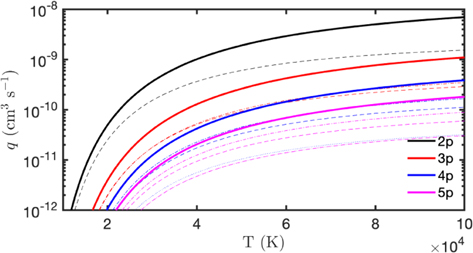
Figure 2. Electron collisional excitation rate coefficients, qij , for 1s →(n, ℓ) transitions of hydrogen derived from collision strengths provided by Anderson et al. (2002). The curves are coded by color (n = 2, 3, 4, 5 as labeled) and by line type (dash–dash 1s-ns, continuous for 1s-np, dashed–dotted for 1s-nd, dotted for 1s-nf, and back to dashdash for 1s-ng.)
Download figure:
Standard image High-resolution imageThe coefficient for energy loss through line X (where, for instance, X denotes Lyα, Hα, 2γ) is given by
where EX is line energy and pk (X) is given in Table 2.
3.1. Simple Fits to Line cooling and Collision Rates
The collisional excitation rate coefficient is the sum over all hydrogen levels,

Both Q(T) and the hydrogen cooling rate (from excitation to n = 2) fall off with temperature as  , where kB
T12 = 3IH/4 is the energy difference between n = 1 and n = 2 levels. We fit the collision rate and ΛH I over two temperature ranges: "hot" (104 K < T < 1.5 × 10⁵ K) and "warm" (104 K < T < 1.5 × 10⁴ K ),
, where kB
T12 = 3IH/4 is the energy difference between n = 1 and n = 2 levels. We fit the collision rate and ΛH I over two temperature ranges: "hot" (104 K < T < 1.5 × 10⁵ K) and "warm" (104 K < T < 1.5 × 10⁴ K ),

where  , as before. A similar expression was derived for ΛH I(T). The fitting parameters for QH I and ΛH I are given in Table 4, and the quality of the fit is displayed in Figure 3.
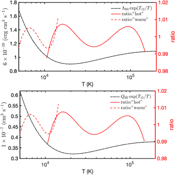
Figure 3. (Top Panel.) Left axis shows the cooling quantity,  , for hydrogen (black line), where the total cooling rate is ne
nH IΛHI(T). These data are fitted to a model described by Equation (5), and the resultig model "fit" parameters are given in Table 4. Right axis shows the ratio, (ΛH I/fit). (Bottom Panel.) The same, but for Q, the collisional rate coefficient. The rate of collisions per unit volume is ne
nHI
Q.
, for hydrogen (black line), where the total cooling rate is ne
nH IΛHI(T). These data are fitted to a model described by Equation (5), and the resultig model "fit" parameters are given in Table 4. Right axis shows the ratio, (ΛH I/fit). (Bottom Panel.) The same, but for Q, the collisional rate coefficient. The rate of collisions per unit volume is ne
nHI
Q.
Download figure:
Standard image High-resolution imageTable 4. Fits to Cooling and Collisional Coefficients
| Quantity | A | a0 | a1 | a2 | a3 |
|---|---|---|---|---|---|
| Λ:hot | 6.0 × 10⁻¹⁹ | 1.018 | −0.335 | 0.290 | −0.059 |
| Λ:warm | 6.0 × 10⁻¹⁹ | 1.032 | −0.494 | 0.637 | |
| Q:hot | 1.0 × 10⁻⁷ | 0.371 | −0.132 | 0.106 | −0.021 |
| Q:warm | 1.0 × 10⁻⁷ | 0.376 | −0.188 | 0.230 | |
Note. "Quantity" refers to the cooling coefficient (ΛH I in erg cm3 s−1) or collisional excitation rate coefficient (QH I in cm3 s−1). These quantities are fitted to a model displayed in Equation (5) over two temperature ranges: "hot" (104 K < T < 1.5 × 10⁵ K ) and "warm" (104 K < T < 1.5 × 10⁴ K.)
Download table as: ASCIITypeset image
We now compute the efficiency of collisional excitations in producing Lyα, Hα, and a 2-photon continuum (each two-photon decay is regarded as one event) as a function of temperature. All inelastic collisional excitations other than to 2s and 2p result in a cascade of photons. The branching ratios are given in Table 2. Both collisional excitation rate coefficients and the branching ratios are used to compute, fX , the number of photons per collisional excitation; here, X = Lyα, Hα and 2γ. These photon yields are plotted in Figure 4. We see that Lyα has the highest yield, approximately 2/3, followed by 2-photon emission, 1/3. Hα is quite weak, even when measured by photons emitted. This is understandable. Hα emission requires excitation to n ≥ 3 levels, whereas two-photon and Lyα emission are obtained by excitation to n = 2 (and also cascade from higher states). However, Hα has a major advantage: it can be observed with existing ground-based observatories.
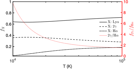
Figure 4. (Left) The run of fX , the photon production per collisional excitation followed by cascades as a function of temperature, T for X = Lyα, X = Hα and X = 2γ continuum. (Right) The ratio, f2γ /fHα as a function of temperature.
Download figure:
Standard image High-resolution imageWe also provide model fits for fX :

where  , as before, and m = 2 or m = 1 (as appropriate). The model fit values are displayed in Table 5. The model fit for Hα is displayed in Figure 5.

Figure 5. (Left axis): The run of fHα , the number of photons produced per collisional excitation, as a function of temperature (black line). A polynomial model for fHα is described in Equation (6) with the coefficients given in Table 5. (Right Axis): The ratio of this model to calculations is displayed by the dashed red line.
Download figure:
Standard image High-resolution imageTable 5. Efficiency of Photons per Collision
| phot | a0 | a1 | a2 |
|---|---|---|---|
| Hα | 0.031 | 0.131 | −0.028 |
| 2γ | 0.378 | −0.042 | |
| Lyα | 0.622 | 0.042 |
Note. Electron collisions with hydrogen atoms produce Lyα, two-photon continuum (2γ), Hα, and other lines. For each of these categories, the efficiency of photon production, f X , depends on temperature and is fitted to a model given by Equation (6). The fit parameters are displayed above. The model is accurate to 2%; see Figure 5 for an example model; th.
Download table as: ASCIITypeset image
4. Electron Collisional Ionization
The collisional ionization rate coefficient is
where f(E) is the Maxwellian energy distribution, IH = 13.598 eV is the ionization energy of hydrogen, and σci (E) is the collisional ionization cross section as a function of electron energy in the center-of-mass frame, E = 1/2μ v2 with μ = me mH/(me + mH) ≈ me . Here, me and mH are the mass of the electron and hydrogen atom, respectively. The collisional ionization rate coefficient can be sensibly written as

Black (1981) provided an approximate form for kci T), based on ionization cross sections tabulated by Lotz (1967),

This expression is consistent with the approximation, σci
∝ (1 − IH/E), quoted in Draine (2011), but only valid at low collision energies (IH ≤ E ≤ 3IH). As shown by Lotz (1967), the high-energy behavior is  . Scholz & Walters (1991) provided a better approximation (for 104 K to 2 × 10⁵ K) using a sixth-order polynomial,

where  . A comparison (Figure 6) between Equation (8) (Black 1981 fit) and the more accurate Scholz & Walters fit (Equation (9)) shows that the former breaks down at high temperatures. We offer a modified formula with the correct asymptotic behavior (kB
T > IH ) as used in the shock models of Shull & McKee (1979),
. A comparison (Figure 6) between Equation (8) (Black 1981 fit) and the more accurate Scholz & Walters fit (Equation (9)) shows that the former breaks down at high temperatures. We offer a modified formula with the correct asymptotic behavior (kB
T > IH ) as used in the shock models of Shull & McKee (1979),
As can be seen from Figure 6, this modified formula provides a good fit at both low and high temperatures. For quick estimates we use Equation (10), but the polynomial formulation of Scholz & Walters (1991; see their Table 2) is preferred when precision is needed (e.g., in numerical integration of differential equations). The resulting ionization power loss per unit volume is ne nH IΛci where Λci = kci IH is the collisional ionization energy loss coefficient.

Figure 6. (Left axis): The run of collisional ionization coefficient (black line) of Scholz & Walters (1991). (Right axis): In red, we plot the ratio of the ionization rate coefficients of Black (1981) from Equation (8) and our handy formula (Equation (10)) to that of Scholz & Walters (1991) labeled  .
.
Download figure:
Standard image High-resolution image5. The Hydrogen Cooling Curve
The goal in this section is to construct a cooling curve for "warm" (T ≲ 105 K) hydrogen plasma. In Section 3 we formulated the cooling coefficient due to line cooling, while in Section 4 we presented the same for ionization losses. Here, we summarize the cooling coefficients for radiative recombination (free-bound) and free–free losses. Armed thus, we formulate the cooling curve for hydrogen in the temperature range 104–105 K.
The kinetic energy of recombining electrons is a loss to the thermal pool. The model fits for radiative effective recombination coefficients αk where k = 1, A, B (corresponding to recombinations to the n = 1s level, and to all states in case A and case B) can be found in Table 7 (Appendix B). The radiative recombination power loss per unit volume is ne np αΛrr where α is either case A or case B, as appropriate. The radiative recombination energy rate coefficient Λrr = α〈Err〉 where 〈Err〉 is the mean thermal energy lost by electron upon recombination. Following Draine (2011) we let 〈Err〉 = frr kB T.
The free–free emission rate per unit volume is ne
np
Λff, where Λff is the free–free emissivity. The free–free power per electron is np
Λff. The mean time for an electron to recombine is  . Thus, the free–free energy lost up to the point of recombination is Λff/α, which we equate to fff
kB
T. The combined recombination and free–free cooling rate coefficient is then
. Thus, the free–free energy lost up to the point of recombination is Λff/α, which we equate to fff
kB
T. The combined recombination and free–free cooling rate coefficient is then

where frf = frr + fff. The run of frf(T) with temperature is displayed in Figure 7 (Appendix B), and the model fits are presented in Table 7 (Appendix B).

Figure 7. (Left): The run of the average kinetic energy of the recombining electron, 〈Err〉, as a function of temperature. (Right): The run of f as a function of temperature (T). The superscripts denote case A or case B. The subscript is "rr" (free-bound radiative recombination), "ff" (free–free emission), and frf = fff + frr.
Download figure:
Standard image High-resolution imageWe now have all the elements to formulate the cooling rate per unit volume,  , expressed as a negative value (for energy losses):

The three RHS terms are given by Equations (3), (7), and (11), respectively.
6. Low-velocity Shocks: A Simple Cooling Model
The investigation of time-dependent cooling of gas heated to T ≈ 105 K is a classic endeavor, constituting the Ph. D. thesis topics of Michael Jura (Jura & Dalgarno 1972) and Minas Kafatos (Kafatos 1973). The motivation in the 1970s seems to have been ambient gas heated by an FUV shock-breakout pulse. Separately, Draine & Salpeter (1978) investigated the production of Lyα from SN shocks, and Shull & Silk (1979) computed UV emission from SNRs in primeval galaxies.
In unmagnetized plasma, assuming a cool (T = 0) pre-shock gas, the post-shock temperature of an adiabatic strong shock (Mach number ≫ 1) is given by
Here, μ is the mean mass per particle and γ is the ratio of specific heats at constant pressure and constant volume; γ = 5/3 for mono-atomic gas. Let y be the number density of helium relative to that of hydrogen. For the gas at the solar circle, y = 0.1. The mean molecular mass for H0 and He0 is μ = [(1 + 4y)/(1 + y)]mH = 1.27mH. It is μ = 0.67mH for H+ and He0, 0.64mH for H+ and He+ and 0.61mH for H+ and He+2.
Three timescales come into play for post-shocked gas: τr , the recombination timescale; τci , the collisional ionization timescale; and τc , the cooling timescale. For gas around 105 K, we have τci ≪ τr . With this inequality, the cooling gas does not obey the conditions for collisional ionization equilibrium. Thus, it is often essential to undertake a full time-dependent calculation.
6.1. Electron-proton Equilibration
At the collisionless shock front, the electrons and protons receive similar amounts of random motion. Being more massive, the protons acquire more energy and are initially much hotter than the electrons. The equilibration timescale for electrons to be heated up to the temperature of the protons via electron-proton encounters is approximately
where  is the Coulomb logarithmic factor accounting for distant encounters (Spitzer 1978; Chapter 2). The current view (Laming et al. 1996; Ghavamian et al. 2007) is that plasma instabilities and electromagnetic waves drive electron-proton equilibration faster than two-body interactions. In Section 6.2 we assume that equipartition occurs before collisional ionization sets in.
6.2. Collisional Ionization
The rate equation for the number density of electrons is

where α = αA , αB as needed. Given our assumption of hydrogen plasma, the number density of protons, np = ne . As noted in Appendix C a solution to this equation at constant T is

Here, x0 = x(t = 0),  and
and  are the characteristic time scales for recombination and collisional ionization, respectively, and

The lowest probable value for the ionization fraction in a realistic diffuse atomic medium, before heating commences, is x0 ≈ 3 × 10⁻⁴. In this case the electrons come from stellar FUV photoionization of C, S, Mg, Si, Fe and other trace metals. As can be seen from Equation (C1) the timescale for electron ionization to reach the half equilibrium fraction is  .
.
6.3. Recombination
As can be seen from Figure 8, collisional ionization is a strong function of temperature. At late times, when the plasma has cooled, collisional ionization can be ignored and Equation (14) simplifies to dx/dt = − x2/τr , with the solution

The ionization fraction decreases from x0 to x0/m on a timescale of t = (m − 1)τr /x0. The run of recombination timescale as a function of temperature is shown in Figure 8.

Figure 8. Ionization time (τci ; see Equation (10)) and recombination time (τr ; case B) as a function of temperature. The two timescales cross at about 15,000 K, at which point the ionization fraction would be 50%, if collisional ionization equilibrium were to hold (see Equation (15)).
Download figure:
Standard image High-resolution image6.4. Basic Cooling and Recombining Framework
The path in the phase diagram of density, ionization fraction, and temperature along which the gas cools depends on the circumstances. For planar radiative shocks, the pressure behind the shock is  , rising to
  downstream when ρ ≫ ρ0. Here, the pre-shock parameters have subscript 0. Thus, radiative shocks are good examples of cooling at nearly constant pressure ("isobaric"). As the gas cools, its density rises to maintain the pressure. A second possibility is cooling at constant density ("isochoric"). The decrease in temperature, following cooling, leads to lower pressure. Pressure changes are conveyed at the speed of sound, cs
. The timescale for adiabatic sound waves to cross a nebula of length L is τa
= L/cs
. Isochoric cooling will take place when the cooling time is short, τc
≪ τa
.
downstream when ρ ≫ ρ0. Here, the pre-shock parameters have subscript 0. Thus, radiative shocks are good examples of cooling at nearly constant pressure ("isobaric"). As the gas cools, its density rises to maintain the pressure. A second possibility is cooling at constant density ("isochoric"). The decrease in temperature, following cooling, leads to lower pressure. Pressure changes are conveyed at the speed of sound, cs
. The timescale for adiabatic sound waves to cross a nebula of length L is τa
= L/cs
. Isochoric cooling will take place when the cooling time is short, τc
≪ τa
.
The first law of thermodynamics states that any gain in the internal energy (U) of the system is due to increase in internal heat and work done: dU = dQ − PdV. For mono-atomic gas, the internal energy of the nebula per unit volume is U = (3/2)nkB T, while the pressure is given by Boyle's law P = nkB T. Here, N = nV is the total number of particles in the nebula whose volume is V. Let NH = nH V be the total number of hydrogen nuclei. Ionization can produce changes in N, whereas NH is fixed.
The three physical parameters governing the cooling hydrogen plasma are ne , T and nH. We have two differential equations, one for ionization balance (ne ; Equation (14)) and one for for energy loss (T; discussed below). A third differential equation follows from the assumed framework: dP/dt = 0 (isobaric cooling) or dV/dt = 0 (isochoric cooling).
For an isochoric system, no work is done by or on the nebula. Adopting case B framework the energy balance equation becomes
where q = 3/2 and the RHS gives the total cooling rate. Note that nH remains constant, whereas n = nH + ne varies as the ionization fraction changes. The ionization-recombination equation (Equation (14)) can be restated
We combine the above two equations to obtain
which we deliberately recast as
In this formulation, the meaning of Equation (16) is clear. The LHS arises from the loss of internal energy. The first term on the RHS represents energy loss from H i collisional line excitation (ΛH I) and collisional ionization (loss of IH per collision). The loss of kinetic energy per recombination (including the free–free radiation up until the recombination event) is given by the second term. The final term accounts for losses/gains to the thermal pool of electrons during recombination and ionization. For plasma in collisional ionization equilibrium this term vanishes, as expected.
For isobaric cooling, the pressure, P = (nH + ne
)kB
T is fixed. In this case, we compute ne
and T and then deduce nH through the pressure equation. As the nebula cools, the ambient gas, in order to maintain the pressure, Pa
, does work on the nebula by compressing the nebula. The work done by the medium on the nebula is PdV. However, since P is constant, d(PV) = Pa
dV. The internal energy of the nebula is then the enthalpy, HV where H = U + Pa
. Going forward, we will drop the subscript to P. It is this store of enthalpy that powers the nebular cooling,  . Since (U + P)V = (5/2)NkB
T we see that Equation (16) still applies but with q = 5/2.
. Since (U + P)V = (5/2)NkB
T we see that Equation (16) still applies but with q = 5/2.
7. Application to a Shock Heated Nebula
Following a strong shock, the density of the post-shock gas density jumps by a factor of four (for mono-atomic gas, as is the case here). As can be seen from Equation (13) the temperature of the post-shock gas depends on the mean molecular weight of the pre-shocked gas. We elect to specify the initial conditions by physical parameters following the shock: post-shock temperature, Ts and post-shock density H-nuclei density, nH. The remaining parameter is the ionization fraction. Radiative shock models show that fast shocks, vs > 110 km s−1, can pre-ionize (H+, He+) the incoming medium (Raymond 1979; Shull & McKee 1979; Dopita & Sutherland 1996). However, here, we consider shocks with velocities below 100 km s−1. Thus, the ionization fraction of freshly shocked gas is the same as the pre-shocked ionization fraction, x0.
Consider a representative post-shock temperature, Ts
≈ 105 K. The electron-proton equilibration timescale will be shorter than  yr (see Section 6.1). The collisional ionization time, tci, is short,
  yr at T = 105 K, rising to
  yr at 50,000 K. Thus, even if the pre-shock gas has minimal ionization (x0 ≈ 3 × 10⁻⁴) it will take a time
  for the ionization fraction to reach half the equilibrium value. The initial losses are large, owing to both collisional ionization and collisional excitation by the newly liberated electrons and subsequent radiation. Once the gas reaches 104 K, forbidden lines of metals will dominate the cooling. The gas will eventually settle down at T1 ≈ 5000–8000 K, the temperature of the stable WNM phase (see Heiles & Troland 2003; Kanekar et al. 2003; Murray et al. 2018; Patra et al. 2018). This WNM layer may develop a WIM layer if sufficient diffuse EUV flux is present.
Ignoring "metals," the mean particle mass is μ = mH(1 + 4y)/(1 + y + x0). The shock velocity and μ determine the post-shock temperature, Ts through Equation (13). Recall that, in our simplified model, the losses from the shocked nebula are only those associated with hydrogen (line radiation, ionization, free-bound, and free–free). In particular, while we include helium in computing the reduced mass, we do not include losses due to helium. In short, we treat helium as a silent and inactive partner. The energy per H-nucleus and associated electron is E0 = qkB Ts (1 + x0 + y). The end state is when hydrogen has largely recombined and thus the energy per H-atom is E1 = qkB T1.
For our fiducial temperature of 105 K, we have E0 ≈ [12.9, 21.5](1 + x0) eV energy per H atom for q = 3/2, 5/2. Thus, on simple grounds, we can see that low-velocity shocks will not significantly affect the ionization of the incoming particles.
7.1. Initial Exploration
We start our investigation by considering two cases, both with post-shock temperature of 1.5 × 10⁵ K and the following parameters: nH = 100 cm−3, x0 = 3 × 10⁻⁴ (indicative of a shock running into CNM; hereafter case "CNM"); nH = 1 cm−3, x0 = 0.5 (indicative of the local ISM ("LISM"; Frisch et al. 2011; Linsky et al. 2022). For each case, under the isobaric framework, we compute the evolution of the physical quantities. We plot the resulting run of temperature, electron density and cooling losses with time in Figures 9 and 10.
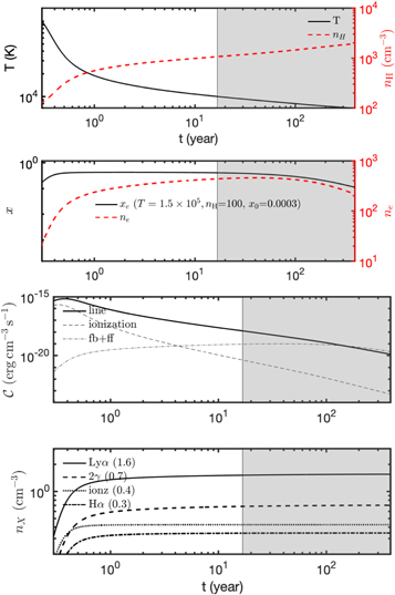
Figure 9. From top to bottom. Panel 1 and 2: Run of temperature (T) and H-nuclei density (nH) of a hydrogen plasma suddenly heated to 105 K and subsequently cooling down via an isobaric process (top-most panel). The run of electron density, ne , and ionization fraction, x, is shown in the next panel down (panel 2). Panel 3 and 4: The run of cooling luminosities (line losses, ionization losses and losses due to free-bound and free–free) as a function of time (panel 3). The run of nX (defined in Equation (17)) vs. T; here c is substituted for X where X is Lyα, 2-photon continuum and Hα (bottom panel; panel 4). For all panels the gray vertical bar represents gas with temperature below 104 K. The calculations stop when the temperature reaches 7000 K.
Download figure:
Standard image High-resolution image
Figure 10. See caption to Figure 9.
Download figure:
Standard image High-resolution imageIn addition to the run of physical quantities (T, x, nH ). we also plot the cumulative number of recombinations per H nucleus,
and the cumulative number of inelastic collisions per atom

where Q(T) is given by Equation (4). A fraction of these inelastic collisions lead to emission of Lyα photons (subscript c=Lyα, nLy ), 2-photon continuum emission (n2γ ), Hα (nHα ) photons and ionizations (ni ).
Radiative recombination also produce Lyα, 2-photon continuum and Hα photons. Draine (2011; Table 14.2) provides, over the temperature range 5 × 10³–2 × 10⁴ K, the recombination coefficients to the 2s level, α2s and for Hα emission, αHα . From these data we find

Thus, at typical temperatures of photoionized gas, recombination results in similar diffuse emission for two-photon continuum and Hα. Separately, αB = α2s + α2p. Thus, 1 − α2s/αB is the fraction of recombinations which result in production of Lyα photons.
From Figure 9 we see that a shock moving into the CNM (with nH = 100 cm-3) cools rapidly. In fact, nominally in less than one year, the post-shocked gas temperature is only 20,000 K. The rapid increase in ionization (panel 2) significantly reduces the proton-ion equilibration time. The strongest energy losses are due to radiative emission (Lyα and 2-photon) followed by loss due to electron collisional ionizations.
Relative to the CNM case, a shock running into the LISM undergoes a slower evolution. At late times (104 yr) as recombination starts the cooling losses mount. This leads to a rapid decrease in temperature and increased recombination. The contribution to the production of line photons (Lyα, 2-photon, Hα) due to electron excitation and recombination is shown in Figure 11. Finally note that, since we are considering low density gas, the photon yields are independent of nH but do depend on Ts and x0.

Figure 11. The run of the cumulative Lyα, 2-photon, Hα yields for the case of shock running into CNM and the local ISM (see caption to Figure 9 and Figure 10).
Download figure:
Standard image High-resolution image7.2. Cumulative Two-photon and Line Yields
A principal goal of the paper is the computation of the number of two-photon decays, Lyα, and Hα per H-nuclei. We distinguish emission due to electron collisions and recombination. The run of these yields as a function of the temperature of the cooling gas is shown in Figure 11. From this figure, we see that the photon "yields" arising from collisions saturate by the time gas has cooled to 104 K, while recombination becomes important only after the temperature has fallen to 2 × 10⁴ K.
These "yields" are a function of shock velocity, vs and initial ionization fraction, x0. In Figures 12 and 13 we plot runs of yields due to collisions ("c:NX " where X = Lyα , Hα , 2γ ) and due to recombination ("r:NX ") as a function of x0 for two representative temperatures.

Figure 12. The run of cumulative yield, NX (X is Lyα, Hα, 2γ decay) by the time gas has cooled to 7000 K as a function of pre-shock ionization fraction, x0 for post-shock temperature of 1.5 × 10⁵ K. The black lines refer to the yields due to electron collisional excitation ("c:") while the red lines due to recombination ("r:").
Download figure:
Standard image High-resolution image
Figure 13. The same as in Figure 12 but for post-shock temperature of 3 × 10⁴ K.
Download figure:
Standard image High-resolution imageIn Table 6 we present the calculations for four post-shock temperatures (1.5 × 10⁴ K, 1 × 10⁵ K, 5 × 10⁴ K and 3 × 10⁴ K) as a function of pre-shock ionization fraction, x0, from 0 to 0.9. Finally, in Figure 14 we display runs of xf, the ionization fraction by the time gas has cooled to 7 × 10³ K.
Table 6. Photon Yields
| Ts | x0 | xf | c:NLyα | c:N2γ | c:NHα | r:NLyα | r:N2γ | r:NHα |
|---|---|---|---|---|---|---|---|---|
| 1.5 × 10⁵ | 0.00 | 0.11 | 1.55 | 0.70 | 0.35 | 0.22 | 0.03 | 0.15 |
| 1.5 × 10⁵ | 0.10 | 0.15 | 1.70 | 0.77 | 0.38 | 0.29 | 0.04 | 0.19 |
| 1.5 × 10⁵ | 0.20 | 0.18 | 1.85 | 0.84 | 0.41 | 0.36 | 0.06 | 0.25 |
| 1.5 × 10⁵ | 0.30 | 0.20 | 2.00 | 0.90 | 0.45 | 0.45 | 0.07 | 0.30 |
| 1.5 × 10⁵ | 0.40 | 0.21 | 2.13 | 0.96 | 0.48 | 0.53 | 0.08 | 0.36 |
| 1.5 × 10⁵ | 0.50 | 0.21 | 2.21 | 0.99 | 0.50 | 0.62 | 0.10 | 0.41 |
| 1.5 × 10⁵ | 0.60 | 0.21 | 2.25 | 1.01 | 0.51 | 0.69 | 0.12 | 0.46 |
| 1.5 × 10⁵ | 0.70 | 0.21 | 2.27 | 1.01 | 0.52 | 0.75 | 0.13 | 0.50 |
| 1.5 × 10⁵ | 0.80 | 0.21 | 2.28 | 1.02 | 0.52 | 0.81 | 0.15 | 0.53 |
| 1.5 × 10⁵ | 0.90 | 0.21 | 2.28 | 1.02 | 0.52 | 0.87 | 0.16 | 0.57 |
| 1 × 10⁵ | 0.00 | 0.05 | 1.06 | 0.50 | 0.22 | 0.11 | 0.02 | 0.08 |
| 1 × 10⁵ | 0.10 | 0.09 | 1.16 | 0.55 | 0.25 | 0.17 | 0.03 | 0.12 |
| 1 × 10⁵ | 0.20 | 0.12 | 1.26 | 0.59 | 0.27 | 0.23 | 0.04 | 0.16 |
| 1 × 10⁵ | 0.30 | 0.15 | 1.36 | 0.64 | 0.29 | 0.30 | 0.05 | 0.20 |
| 1 × 10⁵ | 0.40 | 0.18 | 1.46 | 0.69 | 0.31 | 0.36 | 0.06 | 0.24 |
| 1 × 10⁵ | 0.50 | 0.20 | 1.55 | 0.73 | 0.34 | 0.43 | 0.07 | 0.29 |
| 1 × 10⁵ | 0.60 | 0.21 | 1.65 | 0.77 | 0.36 | 0.51 | 0.08 | 0.34 |
| 1 × 10⁵ | 0.70 | 0.21 | 1.71 | 0.80 | 0.37 | 0.58 | 0.09 | 0.39 |
| 1 × 10⁵ | 0.80 | 0.21 | 1.73 | 0.81 | 0.38 | 0.65 | 0.11 | 0.43 |
| 1 × 10⁵ | 0.90 | 0.21 | 1.73 | 0.81 | 0.38 | 0.71 | 0.12 | 0.47 |
| 5 × 10⁴ | 0.00 | 0.01 | 0.53 | 0.27 | 0.09 | 0.03 | 0.00 | 0.02 |
| 5 × 10⁴ | 0.10 | 0.04 | 0.58 | 0.30 | 0.10 | 0.08 | 0.01 | 0.06 |
| 5 × 10⁴ | 0.20 | 0.07 | 0.62 | 0.32 | 0.11 | 0.14 | 0.02 | 0.09 |
| 5 × 10⁴ | 0.30 | 0.10 | 0.67 | 0.35 | 0.12 | 0.19 | 0.03 | 0.13 |
| 5 × 10⁴ | 0.40 | 0.13 | 0.72 | 0.37 | 0.13 | 0.24 | 0.04 | 0.16 |
| 5 × 10⁴ | 0.50 | 0.15 | 0.76 | 0.39 | 0.14 | 0.29 | 0.05 | 0.20 |
| 5 × 10⁴ | 0.60 | 0.17 | 0.81 | 0.42 | 0.15 | 0.35 | 0.05 | 0.24 |
| 5 × 10⁴ | 0.70 | 0.19 | 0.85 | 0.44 | 0.16 | 0.41 | 0.06 | 0.28 |
| 5 × 10⁴ | 0.80 | 0.20 | 0.90 | 0.46 | 0.17 | 0.47 | 0.07 | 0.32 |
| 5 × 10⁴ | 0.90 | 0.21 | 0.93 | 0.48 | 0.17 | 0.54 | 0.09 | 0.36 |
| 3 × 10⁴ | 0.00 | 0.00 | 0.29 | 0.16 | 0.04 | 0.01 | 0.00 | 0.01 |
| 3 × 10⁴ | 0.10 | 0.03 | 0.32 | 0.17 | 0.04 | 0.06 | 0.01 | 0.04 |
| 3 × 10⁴ | 0.20 | 0.05 | 0.34 | 0.19 | 0.05 | 0.11 | 0.02 | 0.08 |
| 3 × 10⁴ | 0.30 | 0.08 | 0.37 | 0.20 | 0.05 | 0.16 | 0.02 | 0.11 |
| 3 × 10⁴ | 0.40 | 0.11 | 0.39 | 0.21 | 0.06 | 0.21 | 0.03 | 0.14 |
| 3 × 10⁴ | 0.50 | 0.14 | 0.42 | 0.23 | 0.06 | 0.26 | 0.04 | 0.18 |
| 3 × 10⁴ | 0.60 | 0.16 | 0.44 | 0.24 | 0.06 | 0.31 | 0.05 | 0.21 |
| 3 × 10⁴ | 0.70 | 0.18 | 0.46 | 0.25 | 0.07 | 0.37 | 0.06 | 0.25 |
| 3 × 10⁴ | 0.80 | 0.20 | 0.48 | 0.26 | 0.07 | 0.43 | 0.07 | 0.29 |
| 3 × 10⁴ | 0.90 | 0.21 | 0.50 | 0.27 | 0.07 | 0.49 | 0.08 | 0.33 |
Note. The cumulative line and two-photon yields per H-nuclei for post-shock temperature, Ts and initial ionization fraction, x0 computed in the isobaric framework; see caption to Figure 12 for the symbols used for the yields. The calculations are stopped when gas temperature of 7000 K is reached. xf is the ionization fraction at the end of the computations.
Download table as: ASCIITypeset image

Figure 14. The run of ionization fraction of shocked gas, xf, by the time it has cooled to 7000 K as a function of pre-shock ionization fraction, xe for four different temperatures.
Download figure:
Standard image High-resolution image8. Conclusion and Prospects
Shocks with velocities near 70 km s−1 abound in our galaxy. Some descend from higher velocity shocks (e.g., supernova remnants) while others start at low velocity (e.g., stellar bow shocks, high velocity cloud shocks). These shocks do not have strong pre-cursor ionization fronts, and as such the post-shocked gas is partially neutral. Such shocks cool primarily through Lyα, two-photon continuum, Hα, and metal emission lines. Lyα is the brightest line, although resonant scattering traps usually traps these photons within the plasma, resulting in absorption by dust grains. Hα is weak but has the great advantage of being observable from the ground.
Two-photon continuum emission is about 50% of Lyα emission (see Table 6). It is several times brighter than Hα, even when one compares photon fluxes rather than energy fluxes. Fortunately, two-photon emission can be observed with space-based observatories. Furthermore, the two-photon continuum has a distinct FUV/NUV ratio. In fact, GALEX FUV and NUV imagery has led to the recent discovery of large middle-aged supernova remnants (Fesen et al. 2021) and exotic shocked stellar bow shocks with angular scales of hundreds of degrees (Bracco et al. 2020). The Ultraviolet Explorer (UVEX) is a NASA Explorer mission currently under development (Kulkarni et al. 2021). Amongst other goals, UVEX aims to undertake FUV and NUV imaging of the entire sky with higher sensitivity and finer spatial resolution, relative to GALEX. The aforementioned successes with GALEX imagery show great promise of identifying and studying low velocity shocks in a future all-sky survey with UVEX.
With this motivation, and using the best available atomic physics data and atomic calculations, we computed the collisional and cooling coefficients for warm hydrogen (T ≲ 105 K). The primary application of the work presented here is in computing two-photon continuum from bow shocks and old supernova remnants. We allow for pre-ionization by keeping the ionization fraction of the pre-shocked gas as a free parameter that can be set to values computed from more sophisticated shock models (Raymond 1979; Shull & McKee 1979; Dopita & Sutherland 1996). Our expectation is that the accurate H-cooling developed here can be incorporated into time-dependent models (e.g., Gnat & Sternberg 2007).
In the Galactic plane and at low latitudes, two-photon emission will be attenuated by dust in the intervening neutral ISM and contaminated by reflected light from dust grains. In practice, this means that the use of two-photon continuum as a diagnostic will be restricted to high Galactic latitudes and will require careful modeling of reflected light. However, the early successes with GALEX (e.g., Bracco et al. 2020; Fesen et al. 2021) promises rich returns from the planned all-sky FUV & NUV survey of UVEX.
Acknowledgments
We thank Nikolaus Zen Prusinski, California Institute of Technology, for help with CHIANTI, a collaborative project involving George Mason University, the University of Michigan (USA), University of Cambridge (UK) and NASA Goddard Space Flight Center (USA). Partial support was provided to JMS by the astrophysics planning program of New Horizons Extended Mission. We thank the anonymous referee for a most careful reading of our manuscript and excellent suggestions, which resulted in a much better paper.
Appendix A.: Comparison to other Cooling Models
In this section we compare our cooling curve, ΛH I(T), discussed in Section 5, to three notable published curves.
A.1. Scholz & Walters (1991)
Scholz & Walters (1991) provide collisional ionization coefficients (Equation (9)) and total cooling (line and ionization energy losses) coefficients. The latter is given by the following polynomial model:
where T12 = (3/4)TR
with kB
TR
= IH and  . We subtracted losses to ionization, Λci
= kci
IH, to obtain
. We subtracted losses to ionization, Λci
= kci
IH, to obtain  . In Figure 15 we compare our ΛH I(T) (Equation (3)) to
  . The Scholz-Walters curve is systematically lower by 15%. After correction for this scale factor, the two curves agree to within ±5%. Separately, Scholz & Walters (1991) codified the collisional coefficients for excitation from the (1s) ground state of hydrogen to f = 2s and 2p levels

where Γ1s→f is formulated as
In Figure 15 we compare these two coefficients with our own coefficients (Section 3). As with the total line emission cooling, the 2s and 2p collisional rate coefficients are discrepant by the same scale factor.
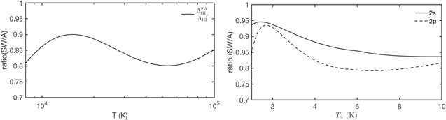
Figure 15. (Left) Comparison of hydrogen line-cooling rate from Scholz & Walters (1991),  given in Equation (A1), with our ΛH I(T) (Equation (3)). The ordinate is the ratio
  . (Right). Comparison of the collisional line excitation coefficients of 1s → 2s and 1s → 2p transitions between Scholz & Walters (1991) ("SW"; see Equation (A2), and the corresponding equation of Anderson et al. (2002) ("A"). The ordinate is the ratio q1s→f
from Scholz & Walters (1991) to that of Anderson et al. (2002).
. (Right). Comparison of the collisional line excitation coefficients of 1s → 2s and 1s → 2p transitions between Scholz & Walters (1991) ("SW"; see Equation (A2), and the corresponding equation of Anderson et al. (2002) ("A"). The ordinate is the ratio q1s→f
from Scholz & Walters (1991) to that of Anderson et al. (2002).
Download figure:
Standard image High-resolution imageA.2. Spitzer (1978)
A classical formula for the volumetric cooling rate of hydrogen plasma is given in Spitzer (1978),  , where

We are aware that our cooling coefficient formulation expresses the line cooling rate per unit volume as ne nH IΛHI. However, there is little difference between our formulation and Spitzer's formulation when the ionization fraction is small. Spitzer's formulation does not include losses from collisional ionization. Spitzer adopted H i cooling rates given in Table 2 of Dalgarno & McCray (1972) which were based on H i excitation cross sections assembled by Gould & Thakur (1970) from theoretical calculations in the 1960s. Those atomic calculations are superseded by more recent work used in this paper (Anderson et al. 2002). In the left panel of Figure 16 we display the ratio of our cooling curves, ΛH I and ΛH = ΛHI + kci IH to the cooling rate of Spitzer (Equation (A3)). Our fit is tuned to be accurate over the range 104–105 K. Even bearing this in mind, it appears that Spitzer's formula over-estimates line cooling at temperatures above 104 K by about 25%.

Figure 16. (Left). The ratio of Spitzer's H-line cooling function to our computations of ΛH I (line cooling) and ΛH (including collisional ionization cooling) as a function of temperature. (Right). Comparison of the total cooling curve (line and ionization losses) between our cooling curve and that from CHIANTI.
Download figure:
Standard image High-resolution imageA.3. Collisional Ionization Equilibrium: CHIANTI
We conclude this section by briefly discussing hydrogen plasma in collisional ionization equilibrium (CIE); electron ionization balanced by radiative recombination. The volumetric cooling rate is given by  where xeq is given by Equation (15). It is mainly dominated by line cooling. CHIANTI (Dere et al. 1997; Del Zanna et al. 2021) is a major resource for astronomers working on collisionally excited gas, especially hot plasma in CIE. CHIANTI returns xeq and cooling function
  (under assumption of case A). Thus, Γ = (1 − xeq)ΛH.
The run of Γ with temperature is displayed in Figure 17. It is evident that Γ from CHIANTI is higher relative to the calculations reported here at higher temperatures. As can be seen from Figure 18 our xeq agrees with that used in CHIANTI for T > 2 × 10⁴ K.

Figure 17. (Left): The run of Γ as obtained from CHIANTI and the calculations reported here (case A, CIE) with temperature T. Here, the ΓCIE is defined as follows:  where it is understood that
  and ne
reflect CIE conditions. (Right): The ratio of Γ (this work) to that reported from CHIANTI.
and ne
reflect CIE conditions. (Right): The ratio of Γ (this work) to that reported from CHIANTI.
Download figure:
Standard image High-resolution image
Figure 18. Left panel: The run of xeq under CIE conditions as a function of temperature, T and the ratio of xeq (this paper) to that provided by CHIANTI. Right panel: The same as the left panel but for 1 − xeq.
Download figure:
Standard image High-resolution imageAppendix B.: Losses Due to Recombination, Free–Free Emission and Ionization
Standard textbooks (e.g., Draine 2011) provide fitting formulae for hydrogen (recombination, free-bound losses) tuned for study of H ii regions. Here, we present fitting formula in the temperature range interest to this paper: 104 K to 105 K. Our starting point is Hummer (1994) who, over an impressive range of 10 K to 107 K, present recombination rate coefficients, αi where i = 1 (recombination to n = 1) and i = A, B for case A and case B; see Figure 19.

Figure 19. Run of H-recombination coefficients (from Hummer 1994).
Download figure:
Standard image High-resolution image
Separately, Hummer (1994) also tabulate the kinetic energy loss due to recombination and free–free emission. In Figure 7 we plot the mean kinetic energy, 〈Err〉 versus T. Note that 〈Err〉 = frr kB T. The resulting fits are presented in Table 7 and are accurate to one percent.
Table 7. Fits to α and f
| qty | A | n | b |
|---|---|---|---|
| α1 | 1.58 × 10⁻¹³ | −0.518 | −0.039 |
| αA | 4.16 × 10⁻¹³ | −0.708 | −0.030 |
| αB | 2.58 × 10⁻¹³ | −0.822 | −0.045 |

| 0.784 | −0.042 | −0.020 |

| 0.672 | −0.109 | −0.021 |

| 1.09 | 0.035 | 0.019 |

| 1.17 | 0.087 | 0.061 |
Note. "qty" is fitted to the model of the form  where the temperature range is 5 × 10³ K < T < 2 × 10⁵ K; here, T4 = T/(104 K). See text for definition of subscripts. The superscripts stand for case A or case B. The unit for α is cm3 s−1 while that for f is dimensionless. The fits are accurate to 1% over the temperature range of interest.
Download table as: ASCIITypeset image
For the free–free emission rate coefficient, Λff we use Equation 10.12 of Draine (2011) to derive fff(T) (see Section 5 for definition of frf ). The values of frf = frr + fff for case A and case B are displayed in Figure 7 (left panel). We assume a simple linear relation and obtain the following fits for frf:
We conclude this section with a discussion of collisional ionization. The energy of the electron, E, upon collision goes into ionizing the atom and imparting kinetic energy to the newly liberated electron. We use the low-energy approximation (Equation (8)) for the collisional cross-section, σci ∝ [1 − (IH/E)] (valid for IH ≤ E ≤ 3IH) to find a mean kinetic energy following ionization,
This formula becomes inaccurate at high temperature (kT ≳ 3IH) where the adopted fit to σci
breaks down (σci
peaks and then falls off as  ). The energy 〈Ek
〉 is shared between the colliding electron and the ionized electron. This energy is not a loss since it is returned to the thermal pool. However, over time, the ionized electron will draw qkB
T energy (q = 3/2 in isochoric framework and q = 5/2 in isobaric framework) from the thermal pool. This is a genuine loss (see the discussion following Equation (16)).
). The energy 〈Ek
〉 is shared between the colliding electron and the ionized electron. This energy is not a loss since it is returned to the thermal pool. However, over time, the ionized electron will draw qkB
T energy (q = 3/2 in isochoric framework and q = 5/2 in isobaric framework) from the thermal pool. This is a genuine loss (see the discussion following Equation (16)).
Appendix C.: Two Solutions to Recombination-Ionization Equation
Equation (14) can be written as

where  is twice the harmonic mean of the two timescales. The equilibrium value for ionization is obtained by setting the LHS to zero, xeq
= τh
/τci
. The above equation can be re-arranged to yield
is twice the harmonic mean of the two timescales. The equilibrium value for ionization is obtained by setting the LHS to zero, xeq
= τh
/τci
. The above equation can be re-arranged to yield

where  . This equation can be integrated using the method of partial fractions to yield
At t = 0,  and thus
This equation is useful to compute the timescale to achieve a particular level of ionization. As t → ∞ , x → xeq , as expected. Alternatively, we apply the transformation, u = 1/x:
Multiply both sides by  to obtain
Because the LHS is the derivative of  , the above equation can be readily integrated to yield

where  and
and  . As t → ∞ , as expected, u−1 → xeq
.
. As t → ∞ , as expected, u−1 → xeq
.
Footnotes
- 4
Only a few stars are likely transiting the Cold Neutral Medium (CNM; 100 K), given its small volume filling factor, ∼1%.
- 5
- 6
A first-order fit would have been sufficient for excitations to all states but 1s-np and 1s-nd. For simplicity, we elected to use the same number of coefficients for all transitions.