
Reason-able embeddings: Learning concept embeddings with a transferable neural reasoner
Abstract
We present a novel approach for learning embeddings of
1.Introduction
In this paper we design, implement and evaluate a novel method of learning concept embeddings in knowledge bases for the
The neural reasoner consists of two modules – a reasoner head, that is a neural network classifier, trained to classify whether subsumption axioms hold for a given knowledge base, and capable of constructing an embedding for arbitrarily complex
In our work we hypothesize, and experimentally show support for the idea that concepts from different knowledge bases can be represented in a shared embedding space, with a topology that lends itself for approximate reasoning by entailment classifiers based on neural networks. This research is a curiosity-driven intellectual endeavor: to the best of our knowledge, this is the first attempt to force a kind of shared semantics on seemingly separate sets of embeddings, yet without defining the semantics explicitly. While we imagine that there may be practical applications of the proposed idea, such as hot-swapping ontologies in a neural-symbolic system, we do not make any claims about its immediate usefulness.
We purposefully limit ourselves to the taxonomical part of
The main contributions of the work are as follows:
– A novel architecture consisting of two parts: a reasoner head, employing a recursive neural network, and a collection of embedding layers. Together, they enable the construction of reason-able embeddings.
– A training procedure employing multiple knowledge bases at once to shape the topology of the embedding space.
– Extensive experimental evaluation aimed at establishing the properties of the proposed approach. In the experiments, we show that the proposed approach indeed forces embeddings to represent the formal semantics in a shared way, that the resulting embeddings are of high quality, and that using this kind of shared, latent semantics does not incur substantial penalty on them.
On top of that, we present three open-source technical contributions implemented in Python that may be useful for the community:
– An implementation of the presented method
– A random axiom generator for the
– An extended interface for the FaCT++ reasoner
Our work is structured as follows. In Section 2, we briefly introduce deep learning (Section 2.1) and description logics (Section 2.2), along with the related notation that we use throughout this text. In Section 3, we give an overview of the current state of the art, in particular of knowledge base embeddings (Section 3.1), and of deep deductive reasoners (Section 3.2). Section 4 presents the details of the architecture for learning reason-able embeddings: in Section 4.1 we present the details of the reasoner head, and in Section 4.2 of the embedding layer. We then introduce a relaxed variant of the architecture in Section 4.3, and describe the training procedure in Section 4.4. The axiom generator for
2.Preliminaries
2.1.Deep learning
While machine learning is ubiquitous in research these days, we give a very brief introduction to ensure there is no confusion in terms. In this, we follow [31], and the reader is welcome to the book for a more extended introduction.
Classification is a task where a learning algorithm is supposed to produce a function, called a classifier, mapping an object to a label from a discrete, finite set of labels. A special case, used in this paper, is binary classification, where only two mutually-exclusive labels are considered: 0 (negative) and 1 (positive). Objects are usually represented by vectors of numerical features, albeit different representations are possible. By convention, features are usually denoted by x, and predicted labels are denoted by
Binary classification is frequently solved by constructing a function predicting the probability of an object to belong to the positive class, and then thresholding on the probability to obtain the label. Throughout this work, we employ this approach, writing
A classifier usually contains a number of parameters, which are automatically adjusted during the training, a process aiming to optimize the value of some metric on a training set. The training set consists of examples, each example being an object assigned a true label that the classifier is supposed to predict. By convention, the true labels are usually denoted as y. The details of the optimization process can vary wildly, but in the context of this work, as the metric we use binary cross-entropy and employ a variant of gradient descent optimization algorithm called AdamW [53] to minimize it.
For gradient descent algorithms, it is established to use a mini-batch training, where the training set is randomly split into small, disjoint subsets called mini-batches, and each mini-batch is used to update the parameters of the model separately. A complete pass over all the mini-batches from a training set is called an epoch. In some special cases, only a subset of parameters is optimized at a given time, while the remaining are called frozen and kept constant.
Due to the stochastic nature of training, too aggressively optimizing the metric can lead to overfitting, a phenomenon in which the classifier labels the training examples very well, but fares poorly on new, unseen data. To evaluate the performance of a classifier on unseen data, a separate set, called test set, is maintained. It is assumed that both sets are independent and identically distributed (the i.i.d. assumption), i.e., the examples in them are drawn independently of each other from the same probability distribution. Usually, for the evaluation, different metrics are used than during training. The details of the metrics used in this paper are given in Section 6.3.
It is frequently the case that a learning algorithm has some configuration options that cannot be automatically adjusted using the training set, e.g., because that would immediately lead to overfitting. These options are called hyperparameters, and are adjusted by observing the value of a metric of choice on yet another set, the validation set. It follows the same i.i.d. assumption as the two other sets.
A feed-forward neural network is a sequence of linear transformations and activation functions, where each transformation is followed by an activation function. By convention, each pair: a linear transformation and an activation function is called a layer. The linear transformation is of form
Over the years, many activation functions were considered. Throughout the paper we use two of them: the sigmoid σ, given in Equation (1), and
Finally, by an embedding we understand a real-valued vector representing some concept from a non-numeric set, such that the size of the vector is much smaller than the cardinality of the set, and that the dimensions are not directly interpretable, i.e., the vector comes from a latent space.
2.2.Description logics
Description logics (DLs) are a family of logics, that are widely used as a formal way to represent knowledge in the form of knowledge bases (KBs). An advantageous property of DLs is that reasoning in most of them is decidable, since they are fragments of first-order predicate logic [1]. The formalism of DLs has been used as a basis for the Web Ontology Language (OWL) standard, which as part of the Semantic Web is responsible for describing the semantics, or meaning, of data on the Internet [59]. DLs and the foundational technologies of the Semantic Web are considered mature, and are used both in research and the industry [36]. An illustrative example of the potential applications of DLs is SNOMED CT – a knowledge base that is considered to be the most comprehensive multilingual clinical healthcare terminology in the world [5].
As mentioned, DLs are a family of logics, which means that there are many DLs of varying expressiveness. Since in our work we focus on the
For readers that are unfamiliar with DLs we begin with an intuitive overview. In later sections we describe the notation we use, and define the syntax and semantics of the
2.2.1.Overview
At a high level, a KB divides knowledge into terminology (also called TBox) and assertions (also called ABox). One may think that the terminology describes general knowledge (e.g. “Dogs are mammals”), and assertions state facts (e.g. “Fido is a dog” or “Fido likes Alice”). Those elements of KB terminology and assertions are called axioms. Axioms are formulated using a vocabulary, which consists of individuals (e.g. “Fido” or “Alice”), concept names (e.g. “dog” or “mammal”), and role names (e.g. “likes”). A concept denotes a set of individuals, and besides concept names in the vocabulary, there are complex concepts that can be constructed from other concepts using concept constructors. The available constructors are different depending on the chosen DL. In particular, in the
The TBox contains subsumption axioms, that allow one to state that one concept is subsumed by another concept. There are two kinds of assertion axioms in ABox: a concept assertion axiom allows one to state that an individual is an instance of a concept, and a role assertion axiom allows one to relate two individuals by a binary role.
Semantics of DLs are defined in a model-theoretic way, by providing an interpretation that represents the KB vocabulary in terms of a set called the domain. In particular, an interpretation maps individuals to elements of the domain, concepts to sets of individuals, and roles to binary relations between individuals. There are also special concepts, called the bottom concept and top concept, which correspond to the empty set and the domain, respectively.
The semantics of DLs provide an entailment relation, so that given a set of axioms, logical consequences may be inferred. In other words, KB entails a given axiom if that axiom follows from KB’s axioms.
2.2.2.Notation
Formally, a KB in the
2.2.3.Semantics
An interpretation is defined as a pair
The set of terminological axioms
The notion can be extended to arbitrary axioms α. We say that α is a logical consequence of
Table 1
Syntax and semantics of
| Description | Syntax | Semantics |
| top | ⊤ | |
| bottom | ⊥ | ∅ |
| intersection | ||
| union | ||
| complement | ||
| existential restriction | ||
| universal restriction |
2.2.4.Ontologies in the web ontology language
While the Web Ontology Language (OWL) is underpinned by a DL, it uses a different nomenclature. In particular, knowledge bases are called ontologies in OWL. We also use the term ontology, but only when referring to a KB described in OWL. Concept names and role names are called class names and object property names, respectively. In general, concepts are referred to as classes or class expressions.
Terminological axioms are called class axioms, and a subsumption
2.2.5.Semantic reasoners
The main benefit of using a knowledge representation paradigm with well-founded semantics is the ability to perform automated reasoning. In this work, we use the entailment checking reasoning task, i.e., deciding whether
Many semantic reasoners for DLs are available, providing reasoning services for KBs, among others, HermiT [61], Pellet [83], and FaCT++ [89] capable of reasoning in very expressive DLs, or more specialized ones such as ELK [44].
In this work, FaCT++ is the reasoner of choice, as it is capable enough to deal with
3.Related work
The neural and symbolic paradigms of artificial intelligence are vastly different. On one hand, the currently dominant neural paradigm shows how well neural networks perform on large-scale data sets, ranging from simple classification and regression, to language models so powerful, that their output is almost indistinguishable from human-written text [9], and generative image models that can synthesize photorealistic images from text prompts [74]. However, neural models often produce nonsensical results, for example paragraphs of text that contradict themselves. Because neural models are not easily interpretable, it is difficult to find the cause of such problems. On the other hand, the symbolic paradigm offers methods for explicitly describing knowledge, and reliably performing reasoning over that knowledge. Symbolic methods can provide step-by-step explanations of their inferences, because they use deductive reasoning. Unfortunately, symbolic methods are not well suited for learning from data, as real-life knowledge is often seemingly contradictory. Symbolic methods also have trouble with processing large-scale data sets, because of high time complexities of used algorithms. The research field of neuro-symbolic integration aims to combine the large-scale learning ability of neural models, and the ability of symbolic methods to express knowledge and perform reasoning, all while keeping interpretability, thus combining the benefits and avoiding the pitfalls of both paradigms [23]. There seems to be two major avenues where the Semantic Web can benefit from the neural paradigm: ontology and knowledge graphs embeddings and deep deductive reasoners [35].
3.1.Knowledge base embeddings
One way to bridge the neural and symbolic paradigms is to represent symbolic knowledge in terms of vectors in a high-dimensional real vector space. Such vectors can then be used as additional inputs to machine learning models based on neural networks, to improve their performance by allowing them to use an approximation of expert knowledge [87]. A good method of learning embeddings from symbolic knowledge should ideally leverage the structural information present in relations between abstract concepts, and should not try to learn embeddings for abstract concepts with the aid of word embeddings, due to the ambiguity of language, its limited abstraction, and other problems [11].
One of the first embeddings methods tailored to KBs to get traction were NTN proposed by Socher et al. [84], TransE proposed by Bordes et al. [7,8], later unified into a single framework by Yang et al. [97], as both leverage linear and bilinear mappings. The notion of modeling relations as operations in some vector space was further extended by Wang et al. with TransH [94], Lin et al. with TransR [51] and PTransE [50], Sun et al. with RotatE [85], Zhang et al. with HakE [98], Wang et al. with InterHT [90], or Zhou et al. with Path-RotatE [99].
A separate category of embeddings was established by ConvE, employing convolutional neural networks [20]. This line of research was continued by Nguyen et al. with ConvKB [62], Jiang et al. with ConvR [42], Demir et al. with ConEx [19]. Over the time even more complex neural architectures were employed, e.g., capsule networks in CapsE by Nguyen et al. [63], recurrent skipping networks by Guo et al. [33], graph convolutional networks in GCN-Align by Wang et al. [93] or R-GCN by Schlichtkrull et al. [82], recurrent transformers by Werner et al. [95]
Yet another approach was taken in RESCAL by Nickel et al. where tensor-based techniques were used [65]. Similar approaches were taken in TOAST by Jachnik et al. [39], TATEC by García-Durán et al. [28], DistMult by Yang et al. [97], HolE by Nickel et al. [64], ComplEx by Trouillon et al. [88], or ANALOGY by Liu et al. [52].
In the context of the Semantic Web technologies, notable examples of embeddings are RDF2Vec by Ristoski et al. [75], OWL2Vec* by Chen et al. [12], and TransOWL by d’Amato et al. [17].
Embeddings are used in various downstream tasks, such as disambiguation [80], ontology learning [71], handling concept drift in streams [13], question answering [54] or fact classification [43]. Over the years multiple survey papers were published on the topic of KB embeddings [10,14,16,91,92].
To the best of our knowledge, none of the proposed methods aims to capture the semantics as a topology of the embedding space, nor enables computing the embeddings of complex expressions from the embeddings of their parts.
3.2.Deep deductive reasoners
Compared to the work on embeddings, much less attention has been devoted to the notion of approximating or emulating the results of deductive reasoning with machine learning, and in particular deep learning [23].
Earlier works, employing traditional machine learning approaches, were mostly devoted to approximate a deductive reasoner in order to obtain the results faster than from a deductive reasoner. For example, Rizzo et al. [76,77] proposed terminological trees and forests to tackle this problem, while Paulheim and Stuckenschmidt concentrated on the problem of approximate reasoning with ABox [70].
One of the first works leveraging deep learning for deductive reasoning over ontologies were those of Makni and Hendler on using recurrent neural networks for RDFS reasoning [56], and of Hohenecker and Lukasiewicz on using recursive reasoning networks [37]. Eberhart et al. employed long short-term memory networks (LSTMs) for reasoning in the
Ebrahimi et al. in [24] introduced a few dimensions along which a reasoner can be classified: logic – which logical formalism is tackled; transfer – the capability of achieving good performance on a previously unknown KB; generative – the capability of generating new inferences, not only answering yes/no queries; scale – the size of considered KBs; performance – high if the system was able to cross the 70% threshold on the F1-score, low otherwise. Following these dimensions, the reasoner presented in this work tackles the
4.Neural reasoner
Fig. 1.
A high-level overview of the neural reasoner architecture. An embedding layer for knowledge base
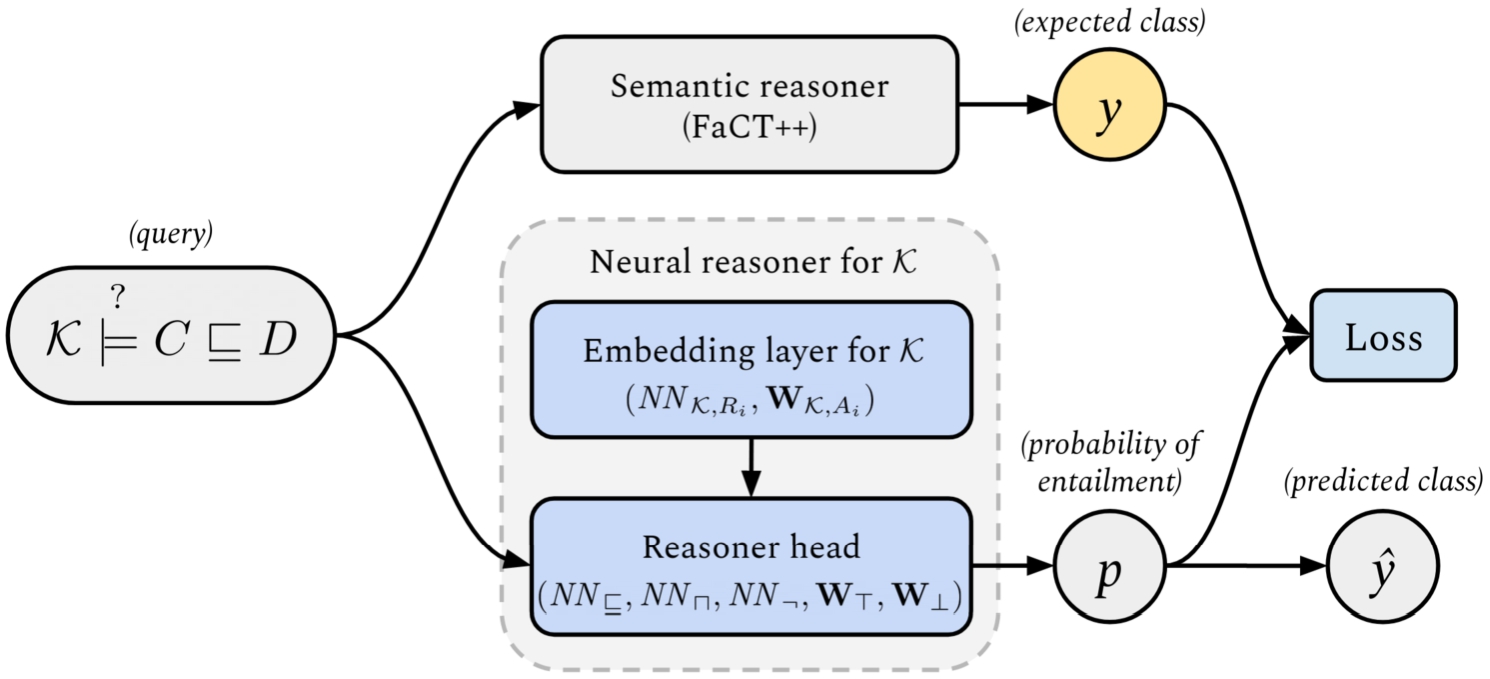
Our neural reasoner (hereafter, reasoner) is a classifier, which given a subsumption axiom, outputs the probability that the axiom is entailed by a given knowledge base. The reasoner consists of the generic reasoner head, and an interchangeable embedding layer specific to a given knowledge base. The generic reasoner head can classify entailment, and construct embeddings for concept complements and intersection of concepts. While an embedding layer contains embeddings for a given knowledge base – that is, it stores embedding vectors for concept names and can construct embeddings for existential restrictions for a given role name. A diagram of the architecture of our neural reasoner is shown in Fig. 1.
The main purpose of the classifier is to facilitate the computation of the gradient of the loss function with respect to the weights of the embedding layer. In other words, when the reasoner is given an axiom, it builds its representation bottom-up from the KB-specific embeddings in the embedding layer. That representation is then used by a neural network in the reasoner head to classify whether the axiom is entailed by that KB. The classification output is contrasted with the target output computed by a semantic reasoner, and the value of the loss function is used to adjust weights of the embedding layer with backpropagation through structure [30].
4.1.Reasoner head
In our work we chose the reasoner to be an entailment classifier for subsumption axioms in
An interaction map for a pair of embeddings u, v, denoted
The classification output for an entailment query
4.2.Embedding layer
Recursive neural networks have been successfully used for encoding expression trees as fixed-size vectors, that could be used as inputs to machine learning models [30]. The recursively defined DL concepts also have a tree structure [49], so it is appropriate to use a recursive neural network as the embedding layer in our reasoner architecture. The key hypothesis that defines our reasoner is that for each KB, we can train an embedding layer that embeds concepts from that KB in an embedding space with a topology that makes it easy for the reasoner head to classify entailment. An embedding topology that is beneficial to entailment classification is formed by jointly training the reasoner head and embedding layers for multiple KBs, which forces the embedding head to generalize, and the embedding layers to output embeddings in the shared embedding space.
We note in passing that we distinguish between a recursive and a recurrent neural network: in a recursive neural network, different parts of the network are applied to the input multiple times, depending on a structured input, as with recursive grammars, where the same production rule can be applied again and again; in a recurrent neural network (e.g., GRU, LSTM) the output of the network is connected back to the network, as part of its input.
In general, concept embeddings are represented by vectors in real vector space
The embeddings of the bottom and top concepts are stored by the vectors
To obtain the embedding for the complement of a given concept, one first recursively obtains the embedding of that concept, and then passes it as an input to the complement constructor network
We also define in Equation (8) the embedding of a doubly negated concept as the embedding of that concept, by the double negation elimination rule, which speeds the construction of embeddings.
To obtain the embedding for an intersection of concepts, one first recursively obtains the embeddings of the two concepts, computes their interaction map, and passes it as the input to the intersection constructor network
Fig. 2.
An example interpretation of a knowledge base with role assertions is shown on the left side. The individuals Fido, Salem, and Rocky are elements of the set
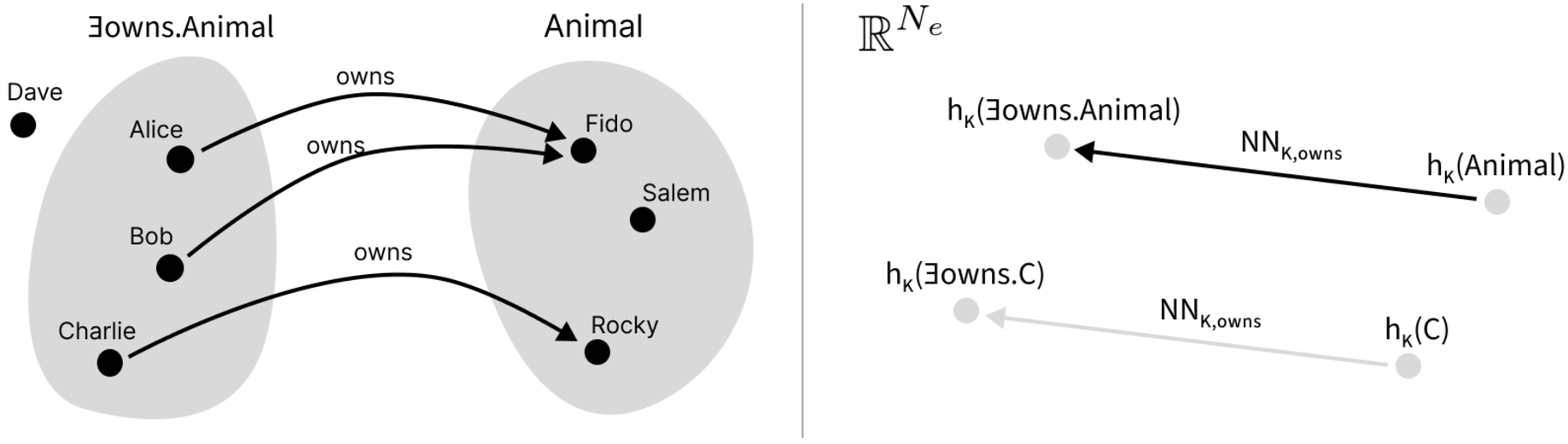
To obtain the embedding for an existential restriction, one first obtains the embedding of the given concept, and passes it to the existential restriction constructor network, defined as
In deep learning, activation functions must be used after each hidden layer so that one does not compose multiple linear transformations, which are equivalent to a single linear transformation. Note that even though our constructor networks do not have an activation function, the result of the
To extend
4.3.Relaxed architecture
An important property of the embedding layer, that we introduced in the previous section, is that the weights of the neural networks
While sharing constructors mimics the logic, it may not be an appropriate assumption in a deep learning model and thus a hindrance to learn good embeddings. To verify whether this is the case, we consider a variant of the reasoner, that allows the embedding layer to learn KB-specific concept constructor networks
In the relaxed architecture, the only weights shared between different KBs are the ones learned by the classifier
4.4.Training procedure
The training procedure for our reasoner consists of two steps. In the first step, we train both the reasoner head and embedding layers for as many diverse KBs as possible. This results in a reasoner head that learned to classify whether subsumption axioms hold in any KB, given that an appropriate embedding layer is provided. By appropriate embedding layer we mean a layer that learned to embed KB-specific concepts in a space that minimizes the classifier loss. We simply call this step training the reasoner head, and we consider the data used in this step as the training set. Note that, as a result of training the reasoner, we obtain trained embedding layers for KBs in the training set. If obtaining the trained embedding layers was the goal, then the next step is not necessary.
In the second step, we freeze the reasoner head and train the embedding layers for KBs that were not seen in the first step. This results in embedding layers that can embed concepts in a space in which the reasoner is good at classification. We think that if our reasoner can accurately classify whether subsumption axioms are entailed by a KB, then the embeddings used as inputs to the classifier
5.Axiom generator
Our reasoner learns embeddings by learning to classify entailment queries
One algorithm for pseudo-randomly generating
Axioms are generated by starting with the grammar rule A (Equation (13)), which returns a subsumption axiom or a disjointness axiom with equal probability. The second alternative is intentionally redundant, to ensure that disjointness axioms are generated frequently enough for the reasoner to benefit from them. Regardless of which alternative was returned, two concepts are generated according to grammar rule C (Equation (14)). First, we select at random the maximum recursion depth for the axiom
The grammar rule C returns one of the following alternatives with equal probability: a concept according to the grammar rule T (Equation (15)), a concept complement, a concept intersection, a concept union, an existential restriction, or a universal restriction. For existential and universal restrictions, the role name
The grammar rule T returns one of the following alternatives: with probability
6.Experimental evaluation
6.1.Goals
Although the design of the proposed approach mimics the
The main hypothesis of our research is that using a transferable reasoner head forces the embeddings to reflect the semantics of the underlying KBs in a shared way. To address it, we pose the following research question RQ1: Can the reasoner induce a useful topology that it can subsequently exploit, or are the embeddings simply overfitting the KBs? We answer RQ1 in Experiment 1, described in Section 6.5, where we compare the classification metrics of a trained reasoner and a random reasoner in previously unseen ontologies, and show that the trained reasoner indeed brings something to the table.
In Section 4.3, we constructed a relaxed variant of the reasoner, hypothesising that the restricted variant may be too restrictive and impede the learning process. From this, we formulate RQ2: Can concept constructors be shared between KBs, or must they be KB-specific? To answer it, we designed Experiment 2, described in Section 6.6. In there, we follow the same procedure as in Experiment 1, but using the relaxed reasoner. We then compare the results obtained by the restricted reasoner in Experiment 1, and by the relaxed reasoner, and show that the difference is negligible.
The overarching goal of this work is to present a method to train embeddings for
We extend RQ1 and RQ3 to a larger set of real-world ontologies, formulating RQ4: Is transfer learning with the presented approach viable for a variety of real-world ontologies? In Experiment 4, described in Section 6.8, we follow the methodology established in Experiment 3 with 6 different ontologies of varying sizes and complexity and show that on average the results of using a pre-trained reasoner head are as good as training a reasoner head from scratch on the considered ontologies.
Finally, we tackle the problem of identifying what is hard for the reasoner by posing RQ5 Are there types of queries that are significantly harder for the reasoner than others?. We briefly address this question in Experiment 5, however, without reaching a satisfactory answer.
6.2.Setup
We implemented the proposed approach in Python 3.9.7 and Cython [4] (a superset of Python that compiles to C or C++), and used PyTorch 1.10.1 to implement the neural reasoner [68]. The source code is available at https://github.com/maxadamski/reasonable-embeddings. We ran the experiments on a computer with an Intel Core i5-4670K CPU, 32 GB of DDR3 RAM, and no dedicated GPU, running Void Linux with kernel 5.15.
We use pseudo-randomly generated numbers to create our data sets and in training. For data generation we use the NumPy implementation of the Permuted Congruential Generator [66]. The internal PyTorch pseudo-random number generator is used during training. To ensure reproducibility of our experiments, we set the initial states of the pseudo-random number generators to a known initial value.
During training, our reasoner uses inferences made by a semantic reasoner as the expected class in classification. The Semantic Web community traditionally uses Java as the language of choice, a language which does not interface well with Python. In particular, using either HermiT [61] or Pellet [83], state-of-the-art semantic reasoners, required executing the reasoners as separate Java Virtual Machine (JVM) processes, a process for every inference. This introduced unacceptable overhead, which we alleviated by employing FaCT++ [89], a semantic reasoner implemented in C++, which makes the task of interfacing with Python much easier. We improved a Python interface for FaCT++ by wrobell,22 extending it with missing concept constructors, and addressing performance issues.
In the experiments dealing with OWL ontologies, initially we used Owlready2 [47] to parse OWL ontologies in the RDF/XML format. Eventually, to improve performance and avoid some problems with the parser, we switched to converting the ontologies to the OWL functional-style syntax [69] using the ROBOT command-line tool [40], and parsing them using a custom, high-performance parser implemented in Cython.
Both our parser and the extended version of the Python interface for FaCT++ are available at https://github.com/maxadamski/reasonable-embeddings/tree/main/src/simplefact, together with compilation instructions in the root of the repository.
6.3.Evaluation metrics
As the quality of the learned embeddings cannot be measured directly, we perform so-called extrinsic evaluation by computing classification metrics for a trained reasoner. We stipulate that if the classification metrics indicate good performance, then the embeddings learned by the embedding layer must capture the semantics of a given KB well. If that was not the case and the embeddings did not encode useful information for inference in the
For simplicity, in threshold-sensitive metrics we choose a threshold of 0.5, i.e,
Our classifier learns binary classification, so we chose appropriate metrics [86]. Firstly, we include accuracy (Equation (16)) in the set of evaluation metrics. Because the data set that we generated for the experiments is slightly imbalanced we also compute precision (Equation (17)), recall (Equation (18)), and the F1-score (Equation (19)).
We also compute the values of the area under the ROC curve (AUC-ROC) and the area under the PR curve (AUC-PR), which are threshold-invariant metrics with a minimum value of 0 and a maximum value of 1. The ROC curve shows the performance of a classification model at all classification thresholds, by plotting the true positive rate (TPR; also called recall) against the false positive rate (FPR) (Equation (20)). Similarly, the PR curve shows the performance of a model at all thresholds by plotting precision against recall [79]. For both ROC and PR curves, a larger area under the curve suggests a better classifier [26,79].
In experiments leveraging multiple KBs, we compute all metrics separately for each query set, and then compute the average and standard deviation across KBs. We do this because the KBs in the test set may be unequally difficult to classify, so it is beneficial to measure the variance of the reasoner performance across different KBs.
6.4.Data sets
6.4.1.Synthetic data set
Finding a large number of
For each KB, we also randomly choose the number of terminological axioms
For each knowledge base
We assign the first 40 KBs as the training set and the remaining 20 KBs as the test set. We then create a validation set from 20% of the queries from the training set. In total, there are 64,000 queries in the training set, 16,000 queries in the validation set, and 40,000 queries in the test set. In every data set, approximately 21.5% of queries have class
6.4.2.Data set of real-world ontologies
Preprocessing We do the following pre-processing steps to make OWL ontologies compatible with our reasoner. Pre-processing is done automatically after parsing the ontology file, so one does not need to edit the ontology manually.
– We ignore object property axioms, since role axioms are not expressible in
– We ignore axioms with number or value restrictions, since they are not expressible in
– We ignore individuals and ABox axioms, since our reasoner does not support ABox reasoning.
– We remove roles that do not appear in any TBox axiom kept after pre-processing. This is done because of a limitation in FaCT++, which makes it raise an exception, when constructing a concept with an unused role name.
The pizza ontology We use the pizza ontology33 from the Manchester University OWL Tutorial [38] We chose the pizza ontology, because it has a similar number of axioms, concept and role names to the randomly generated KBs from the synthetic data set.
The ontology contains 99 classes and 8 object properties, which are equivalent to concept names and role names, respectively. There are 15 equivalence axioms and 15 class disjointness axioms. Two of the classes are unsatisfiable.
The preprocessing is not without some influence on the ontology: InterestingPizza is equivalent to the top concept, because the axiom defining it as a pizza with at least 3 toppings contained a number restriction, so it was removed. The equivalence axiom that defines RealItalianPizza as a pizza with Italy as its country of origin was removed because it contained a value restriction. Since RealItalianPizza was also defined as a subclass of
CQ2SPARQLOWL To further test the capabilities of our architecture, we use the set of ontologies accompanying the CQ2SPARQLOWL data set44 [73,96]. It consists of five ontologies:
– Software Ontology55 (SWO) with 4068 classes, 52 object properties and 7683 axioms [57]
– Stuff ontology66 (Stuff) with 193 classes, 57 object properties and 717 axioms [45]
– African Wildlife Ontology77 (AWO) with 31 classes, 5 object properties and 56 axioms [46]
– Dementia Ambient Care ontology88 (Dem@Care) with 261 classes, 72 object properties and 695 axioms [18]
– Ontology of Datatypes99 (OntoDT) with 406 classes, 16 object properties and 947 axioms [67]
The ontologies were preprocessed according to the procedure described earlier.
6.5.Experiment 1 – topology induction on the synthetic data set
In this experiment, we consider RQ1: Can the reasoner induce a useful topology that it can subsequently exploit, or are the embeddings simply overfitting the KBs? To answer it, we designed a simple test to check whether a trained reasoner head actually learns to reason in the
We test our architecture by first training the reasoner head and embedding layers on the training set (as usual), which results in a skillful reasoner. Then we create a no-skill reasoner head, that is not trained, but only randomly initialized. For each of the two reasoner heads, we train embedding layers on the test set, but keep the reasoner head weights frozen. After training the embedding layers on the test set for a fixed number of epochs, if the classification metrics for the reasoner with the trained head are significantly greater than for the reasoner with the random head, then the trained reasoner head learned useful relations in the
Conversely, if the differences between classification metrics of both reasoner heads are not significant, then the trained reasoner actually has little or no skill and the only skill in classification comes from the embedding layer, which would mean that the reasoner head is not transferable.
6.5.1.Training details
The embedding dimension is set to
We train both reasoner variants with mini-batch gradient descent for 15 epochs, which was enough for the validation loss to stop decreasing. During testing, we train the embedding layers (while the reasoner head weights are frozen) for 10 epochs, as the test loss stabilized after that. We set the batch size to 32, as small batch sizes have been shown to improve generalization [58]. Unless stated otherwise, all weights are randomly initialized using the Xavier initialization [29].
6.5.2.Evaluation of reasoning ability
We evaluate the reasoning ability of the restricted variant of our reasoner by monitoring the training and validation loss and AUC-ROC values during training. The only goal of this assessment is to verify that the reasoner can effectively learn to classify entailment in the training set, and does not suffer from underfitting. Training and validation losses steadily decreasing, and validation AUC-ROC increasing with each training epoch, suggests that the reasoner architecture is sufficient for learning to classify entailment in a given data set.
Fig. 3.
Training and test progress of the restricted reasoner. The reported training loss for each epoch is the average mini-batch loss in that epoch. We also show the standard deviation of the mini-batch loss for each epoch. In test progress, the trained reasoner is shown in red, while the random reasoner is shown in blue. The reasoner was not trained during epoch 0 of training and testing – during epoch 0 we only compute the initial loss and metric values. Dashed curves show the AUC-ROC for each KB in the test set, while the thicker blue and red curves are the averaged AUC-ROC across KBs in the test set. Note that the random reasoner loss actually decreases, but at a very slow rate.
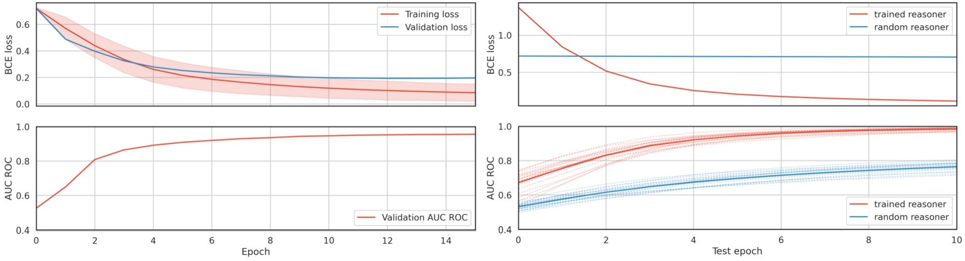
As shown in Fig. 3, the training loss decreases and validation AUC-ROC increases for the entirety of the training, with smaller gains after epoch 10. Furthermore, the validation loss does not start increasing in later epochs, which suggests that the restricted reasoner variant is not prone to overfitting.
6.5.3.Evaluation of knowledge transfer
After training the restricted reasoner, we froze the reasoner head, and trained embedding layers on the test set. We also trained separate embedding layers in conjunction with a randomly initialized, frozen reasoner head. The test loss decreased quickly for the reasoner with the trained head, while the loss for the random head decreased so slowly, that the test loss curve seems stationary on the plot. For the reasoner with the trained head, the test AUC-ROC quickly increased to almost 0.8 after epoch 2, and approached 1 after the last epoch.
Overall, training embedding layers for the reasoner with the trained head was much faster, than for the reasoner with the randomly initialized head, as the reasoner with the trained head achieved average AUC-ROC greater than 0.8 after epoch 2, while it took the reasoner with the random head 10 epochs to do the same. Furthermore, the trained head allowed the reasoner to achieve an average AUC-ROC close to 1 on the test set after 10 epochs, while the reasoner with the random head only achieved an average AUC-ROC of around 0.8.
The metrics after the last training epoch on the test data are reported in Table 2. The extremely high recall of the reasoner with the randomly initialized head is an artifact of it classifying most queries as class 1. Given the very low precision of the reasoner with the random head, its high recall should be ignored. The restricted reasoner with the trained head has lower variance of AUC-ROC and accuracy, than the reasoner with the random head. However, the restricted reasoner with the random head has lower variance for the F1-score, precision and recall. The trained reasoner outperforms the random reasoner on all measures except recall.
Table 2
Test set metrics for the restricted reasoner. Metric values were averaged across different KBs in the test set. In addition to averages, we standard deviation values are shown
| Model | Accuracy | Precision | Recall | F1 | AUC-ROC | AUC-PR |
| Trained head | ||||||
| Random head |
6.5.4.Measuring the effect of embedding size and reasoner head width on performance
Table 3
Test set metrics for the restricted reasoners with varying embedding size (
| k | Accuracy | Precision | Recall | F1 | AUC-ROC | AUC-PR | |
| 1 | 1 | ||||||
| 16 | 1 | ||||||
| 1 | 10 | ||||||
| 16 | 10 |
To determine the effect of the embedding size and the number of neurons in the reasoner head we set the embedding size to 1 and/or the number of neurons to 1, and repeated the training procedure we described earlier. A reasoner with 1 neuron is a linear classifier and thus must rely on the embeddings to convey almost all the necessary information. Conversely, an embedding of size 1 is sufficient if all the necessary information is stored in the reasoner.
We report the results in Table 3. Following [41], we used repeated measures ANOVA on the AUC-ROC and obtained a p-value below 0.001, i.e., for at least one pair
The variant with
Answering RQ1, the presented results indicate that the reasoner indeed shapes the embedding space and generalizes well to previously unseen KBs, not storing any substantial amount of knowledge.
6.6.Experiment 2 – comparing restricted and relaxed reasoners
In this experiment we answer RQ2: Can concept constructors be shared between KBs, or must they be KB-specific? We followed the same protocol as in Experiment 1, but used the relaxed reasoner instead of the restricted reasoner.
6.6.1.Evaluation of reasoning ability
First, we trained the relaxed reasoner on the training set. The training progress for this variant is shown in Fig. 4. The training loss decreases and the validation AUC-ROC increases for the entirety of the training, with smaller gains after epoch 10. The validation loss decreases until epoch 10, and then starts increasing, which indicates overfitting.
When comparing Fig. 4 with Fig. 3, we observe that the AUC-ROC metric for the validation set increases slower for the relaxed reasoner than for the restricted reasoner. We attribute the faster convergence to the shared concept constructor networks
6.6.2.Evaluation of knowledge transfer
Fig. 4.
Training and test progress of the relaxed reasoner. The reported training loss for each epoch is the average mini-batch loss in that epoch. We also show the standard deviation of the mini-batch loss for each epoch. In test progress, the trained reasoner is shown in red, while the random reasoner is shown in blue. The reasoner was not trained during epoch 0 of training and testing – during epoch 0 we only compute the initial loss and metric values. Dashed lines show the AUC-ROC for each KB in the test set, while the thicker blue and red curves are the averaged AUC-ROC across KBs in the test set.
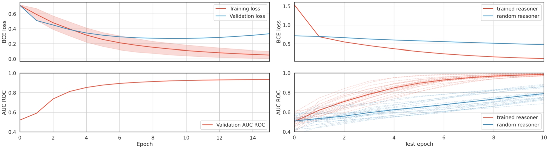
After training the relaxed reasoner, we froze the reasoner head, and trained embedding layers on the test set. We also trained embedding layers in conjunction with a randomly initialized reasoner head. The test progress is shown on the right side of Fig. 4. At the beginning, the test loss for the trained reasoner head was higher than the test loss for the randomly initialized reasoner head. The test loss decreased quickly for the reasoner with the trained head, while the loss for the random head decreased very slowly. For the reasoner with the trained head, the test AUC-ROC quickly increased to about 0.7 after epoch 2, and approached 1 after the last epoch. The average test AUC-ROC for the random head slowly increased from around 0.5 in the beginning to around 0.8 after the last epoch.
Overall, training embedding layers for the relaxed reasoner with the trained head was much faster, than for the reasoner with the randomly initialized head. Moreover, the trained head allowed the reasoner to achieve an average AUC-ROC close to 1 on the test set after 10 epochs, while the reasoner with the random head only achieved an average AUC-ROC of around 0.8.
We report the final metrics of training on the test data in Table 4. For the relaxed architecture, the trained model is strictly better than the randomly initialized one, as all metric values are higher for the former. Moreover, the trained model has lower variance of metrics across KBs in the test set, than the random model. Similarly as for the restricted reasoner, the reasoner with trained head outperforms the reasoner with random head by a fair margin.
6.6.3.Comparative results
Comparing the metrics for the restricted reasoner in Table 2 and for the relaxed reasoner in Table 4, we observe that as expected, for both relaxed and restricted reasoners, the reasoners with trained heads achieved superior performance on the test set, which shows that both variants are indeed transferable.
Between the two random reasoners, the relaxed variant achieves better metric values, except recall, due to the very high recall of the restricted random reasoner. This was expected, since in the relaxed variant, the complement and intersection constructor networks can adjust to the randomly classifier to minimize the classification error, while in the restricted variant this is not possible.
Table 4
Test set metrics for the relaxed reasoner. Metric values were averaged across different KBs in the test set. In addition to averages, the standard deviation values are shown
| Model | Accuracy | Precision | Recall | F1 | AUC-ROC | AUC-PR |
| Trained head | ||||||
| Random head |
When comparing the trained reasoners, the relaxed variant achieves slightly higher values with lower variance for all metrics (except precision, for which the restricted variant has slightly lower variance). However, the differences are not statistically significant. For each metric, we conducted a paired t-test, and checked whether the metric values for KBs from the test set, do not significantly differ between the relaxed and restricted reasoners. The resulting p-values, shown in Table 5, indicate that the null hypothesis cannot be rejected for any metric, even on a relatively high significance level
Table 5
p-Values of the t statistic in a paired t-test for the test set metrics of a trained restricted reasoner and trained relaxed reasoner
| Accuracy | Precision | Recall | F1 | AUC-ROC | AUC-PR | |
| p | 0.1798 | 0.4431 | 0.0801 | 0.1529 | 0.9236 | 0.8399 |
Disregarding the performance metrics, the restricted reasoner has an advantage over the restricted reasoner – it has fewer learnable parameters. Since one of the main goals of our reasoner is transfer learning, a lower number of parameters in the embedding layer is preferable, as it speeds up training for new KBs. The average embedding layer training time per epoch was approximately 21.72 seconds for the restricted variant, and 26.84 seconds per epoch for the relaxed variant, which is 23% slower.
Answering RQ2, introducing restrictions does not significantly change the reasoning performance, as measured by the classification metrics, but increases training efficiency.
6.7.Experiment 3 – visualizing concept embeddings from a real-world ontology
The previous experiments showed that our reasoner is capable of learning good concept embeddings for synthetic KBs, so the next step is to answer RQ3: Can the presented approach learn good embeddings for concepts from a real-world ontology? In this experiment we do that by training the neural reasoner to classify entailment, given randomly generated queries about the pizza ontology as the data set. We repeat this experiment three times. In the first run, we let the reasoner learn without any pre-training. In the second run, we initialize the reasoner head with weights of the restricted reasoner, that we trained in Experiment 1, then freeze it, and only allow the embedding layer to learn. In the third run, we randomly initialize the reasoner head, and also freeze it to only allow the embedding layer to learn KB-specific embedding.
6.7.1.Training set
The data set for this experiment consists of 32,000 unique random queries that we generate using the algorithm described in Section 5. We set the maximum axiom depth to
6.7.2.Training procedure
As mentioned, we repeat learning three times, which results in three reasoners:
– Reasoner with unfrozen head – Both the reasoner head and embedding layers were trained.
– Reasoner with frozen pre-trained head – Only embedding layers were trained. The reasoner head was initialized with the weights of the restricted reasoner, that we obtained in Experiment 1.
– Reasoner with frozen random head – Only embedding layers were trained. The reasoner head was initialized randomly and its weights were immediately frozen.
In every run of the experiment we trained the model for 30 epochs, with learning rate set to
We expected the reasoner with the unfrozen head to achieve the best metric values and learn the best embeddings out of the three reasoners in the embedding analysis, because no weights are frozen, which means that the reasoner with the unfrozen head can fit to the data set more than the reasoners with frozen heads. The only obstacle to learning good embeddings for the reasoner with unfrozen head are the randomly generated queries, that may not contain useful entailments for the pizza ontology, although the other two reasoners learn with the same data set, so the comparison is at least fair.
Based on the results of Experiment 1, we expected the reasoner with transfer to achieve higher classification metrics than the reasoner with randomly initialized frozen head. In Experiment 1, the trained reasoner head was better at classifying queries for the unseen KBs from the test set, than the randomly initialized reasoner head, so we expected the same to be true for the pizza ontology.
6.7.3.Evaluation of reasoning ability
Table 6
Classification metrics for reasoners in Experiment 3 after training for 30 epochs
| Reasoner head | Accuracy | Precision | Recall | F1 | AUC-ROC | AUC-PR | Training time |
| Unfrozen | 0.9929 | 0.9897 | 0.9930 | 0.9914 | 0.9996 | 0.9995 | 411.16 s |
| Frozen pre-trained | 0.9527 | 0.9508 | 0.9331 | 0.9419 | 0.9859 | 0.9823 | 354.99 s |
| Frozen random | 0.7733 | 0.6593 | 0.9283 | 0.7710 | 0.8932 | 0.8390 | 328.49 s |
The classification metrics of the three reasoners are shown in Table 6. As expected, the unfrozen reasoner achieves strictly better classification performance than the reasoners with frozen heads, as the values of all metrics are higher than for other reasoners. The reasoner with the frozen pre-trained head is the second-best reasoner after the unfrozen reasoner, and is strictly better than the reasoner with the randomly initialized head.
The reasoner with the randomly initialized frozen head was the worst of the three reasoners, although it is better than a random guesser, with AUC-ROC of around 0.90. This reasoner has very high recall, but relatively low precision, which is reflected in the significantly lower F1-score and AUC-PR, when compared to the better reasoners. Even though the reasoner with the randomly initialized head was the worst of the three, it still achieved relatively high metric values, which shows that good embeddings can compensate for a bad reasoner head.
6.7.4.Evaluation of knowledge transfer
In the last section, we discussed the differences between the three reasoners that we trained in Experiment 3. Taking into account the differences between the reasoners with frozen heads, we conclude that the transfer of knowledge from the randomly generated KBs in Experiment 1 to the pizza ontology was a success. The reasoner with the pre-trained head achieved results similar to the unfrozen reasoner, which is very promising, given that the pizza ontology is certainly different from the randomly generated KBs used as the training set in Experiment 1.
It should be mentioned that the total training time of the reasoners with frozen heads is shorter than the training time of the unfrozen reasoner, which is the case because there is no time spent on updating the reasoner head weights.
6.7.5.Embedding analysis
In addition to evaluating the reasoning and transfer ability of our reasoner, which showed that it can successfully learn to classify entailment in a real-world KB, we visualize the learned embeddings. A 2D visualization that tries to preserve the distances between concepts in the high-dimensional embedding space enables visual assessment of the quality of the learned embeddings. We think that if semantically similar concepts are placed closer to each other than to dissimilar concepts, then the learned embeddings capture the semantics of a given KB.
We set the concept embedding dimension to
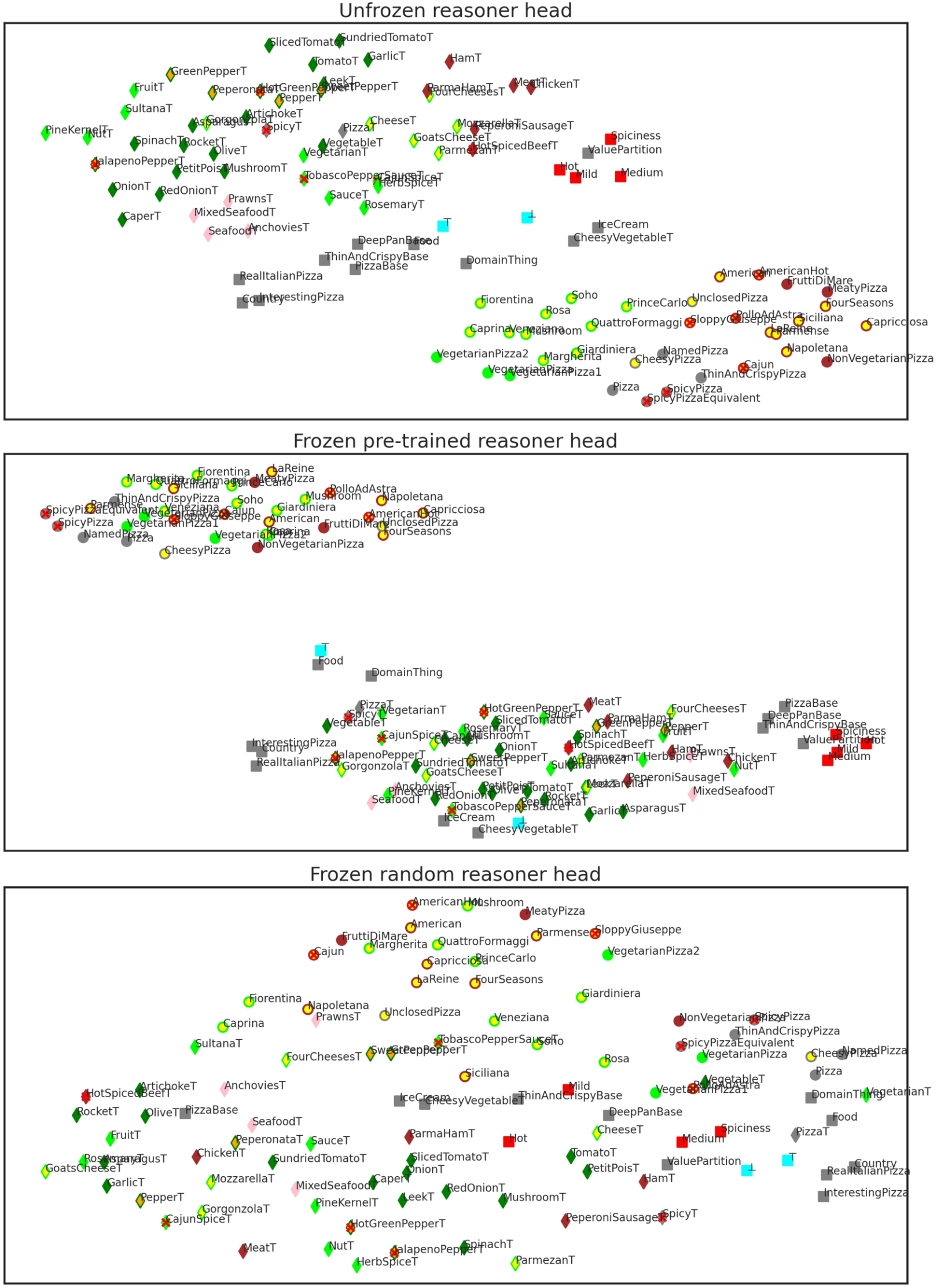
The UMAP visualizations of the embeddings learned in this experiment, are shown in Fig. 5. The visualization of embeddings learned by the unfrozen reasoner suggests, that the embeddings capture the semantics of the pizza ontology well. As expected, the unsatisfiable CheesyVegetableTopping is close to ⊥, and the general DomainThing and Food concepts are close to ⊤. Spiciness and pizza bases form their own clusters. Pizzas and toppings are separated, with vegetarian pizzas forming one cluster, and non-vegetarian pizzas forming another cluster together with spicy pizzas. Cheesy toppings, vegetable toppings, spicy toppings, and pepper toppings are also close to related concepts.
The embeddings learned by the reasoner with the pre-trained head look a bit worse than those of the unfrozen reasoner. The pizzas and the toppings are separated, but inside of the topping and pizza clusters the embeddings are not as well organized.
The embeddings learned by the reasoner with the randomly initialized head do not look good when visualized. A few concept names form clusters that make sense, but most look like they are randomly scattered. General concepts are close to the top concept, which is good, but the unsatisfiable CheesyVegetableTopping is far away from the bottom concept.
In general, we think that the embeddings for the unfrozen reasoner are the best, the embeddings for the reasoner with the frozen pre-trained head are good, and the embeddings for the reasoner with the frozen randomly initialized head are not good at all. Again, the results of the visual assessment of the learned embeddings are consistent with the classification metrics of the reasoners.
Overall, the presented results indicate that the answer to RQ3 is affirmative, and that the presented approach can learn embeddings of good quality.
Fig. 5.
UMAP visualization of the learned concept embeddings. We replaced “Topping” in concept names with “T” to improve readability. We use different shapes, sizes, and colors of markers as follows: by default concepts are square and gray; the top concept, bottom concept and concept expressions are cyan; toppings diamond-shaped, and pizzas are round; vegetarian pizzas and toppings are light green, except vegetable toppings, which are dark green; seafood toppings are pink; non-vegetarian pizzas and meat toppings are dark red; cheesy pizzas, and cheese toppings are respectively marked with a yellow disk or yellow diamond inside; pepper toppings are marked with an orange diamond inside; spicy things are marked with a red “x” inside; spiciness levels are light red.
6.8.Experiment 4 – learning concept embeddings in different real-world ontologies
In Experiment 3 we found that a reasoner with a frozen pre-trained head achieves similar classification metrics to a reasoner trained from scratch. To see whether this result holds for a more diverse set of ontologies we posed RQ4: Is transfer learning with the presented approach viable for a variety of real-world ontologies?
6.8.1.Training set
In this experiment we use six real-world ontologies: five ontologies from the CQ2SPARQLOWL data set, and the pizza ontology. For each ontology, we generate 32,000 unique random queries according to the algorithm described in Section 5. We set the maximum axiom depth to
6.8.2.Training procedure
Similarly to the Experiment 3, we repeat learning three times, which results in three reasoner heads, each with six embedding layers.
– Reasoner with unfrozen head – Both the reasoner head and embedding layers were trained.
– Reasoner with frozen pre-trained head – Only embedding layers were trained. The reasoner head was initialized with the weights of the restricted reasoner, that we obtained in Experiment 1.
– Reasoner with frozen random head – Only embedding layers were trained. The reasoner head was initialized randomly.
We use the exact reasoner architecture and training setup as in Experiment 3, but in this experiment each mini-batch could contain queries for any of the six ontologies, as the embedding layers were trained in parallel.
6.8.3.Results
The metric values for the pizza ontology are slightly different from the ones in Experiment 3, as this time, the reasoner head was trained on six ontologies at once, in contrast to exclusively training on the pizza ontology. We report the classification metrics for each reasoner head, averaged over all ontologies, in Table 7, and we give the values for each ontology separately in Appendix A.
Table 7
Classification metrics for reasoners for the AWO, Dem@Care, Stuff, SWO, OntoDT, and Pizza ontologies. Values were averaged over all ontologies
| Reasoner head | Accuracy | Precision | Recall | F1 | AUC-ROC | AUC-PR | Train time |
| Unfrozen | 27 min 18 s | ||||||
| Frozen pre-trained | 24 min 6 s | ||||||
| Frozen random | 24 min 5 s |
In Table 8 we report the p-values obtained from a paired t-test between the unfrozen head, and the frozen pre-trained head. As some of the p-values hint on the possibility of statistical significance, we also report the adjusted p-values
The results indicate that using a pre-trained head is a viable choice for real-world ontologies, as the performance drop is negligible, and thus the answer for RQ4 is positive.
Table 8
p-Values of the t statistic in a paired t-test for the test set metrics of a reasoner with an unfrozen head and a frozen pre-trained head. Adjusted p-values
| Accuracy | Precision | Recall | F1 | AUC-ROC | AUC-PR | |
| p | 0.0338 | 0.0432 | 0.0319 | 0.0277 | 0.0208 | 0.0335 |
| 0.1383 | 0.1383 | 0.1383 | 0.1383 | 0.1244 | 0.1383 |
6.9.Experiment 5 – what is difficult for the reasoner?
One can wonder what types of axioms are particularly hard for the reasoner. To answer this, we started with the reasoner and the test set from Experiment 1. Then, for each query in the test set, we computed the following features:
–
–
–
–
–
–
– d – the depth of the syntax tree of the query (i.e., the recursion depth d as defined in Section 5);
Table 9
The Pearson correlation coefficient between each feature and the classification error of the reasoner
| d | ||||||
| −0.0106 | −0.0051 | −0.0062 | −0.0015 | 0.0282 | 0.0004 | −0.0065 |
Currently, we do not have a decisive answer to RQ5. There do not seem to be any obvious indicators of hardness for a query. We stipulate it might be possible to detect more complex patterns by using, e.g., an adversarial attack [32], or frequent pattern mining [48,72]. However, we deem this to be out of the scope of this work.
7.Conclusions
In this work, we introduced a novel method of learning data-driven concept embeddings, called reason-able embeddings, in
We also show that using recursive neural networks for constructing embeddings of arbitrarily complex concepts obviates the need for manually designing concept vectorization schemes, and avoids the pitfalls of recurrent neural networks operating on a textual representations of concepts. Instead, concept embeddings can be learned in a data-driven way, by simply asking entailment queries for a given knowledge base.
Finally, we show that a significant part of our reasoner is transferable across knowledge bases in the
We hope that our neural reasoner architecture will allow for greater use of knowledge in models based on neural networks, both by providing an effective way of learning concept embeddings, and learning an accurate entailment classifier for knowledge bases in description logics, thus, making a small step towards the integration of the neural and symbolic paradigms in artificial intelligence.
We identified many opportunities to improve, extend and apply our neural reasoner, that were out-of-scope for this work, but look like promising avenues for future research. In our work we used small neural networks, but deeper and wider concept constructor networks, and subsumption entailment classifier networks could be examined. The number of parameters in the reasoner could also be reduced, while preserving the quality of embeddings and accuracy of entailment classification. Currently, the number of parameters scales quadratically with the embedding dimension, because the reasoner uses the outer product of embeddings as an input to neural networks
Finally, it would be interesting to see if recursive neural networks could be applied in reverse to how we use them – to generate concepts, given learned concept embeddings. That would make it possible to not only learn concept embeddings by classifying entailment, but also to induce new concepts by sampling the embedding space, e.g., to construct a scalable algorithm for explainable artificial intelligence [81].
Notes
1 Each element of the outer product of two vectors
3 The pizza ontology in the RDF/XML format is available at http://owl.cs.manchester.ac.uk/publications/talks-and-tutorials/protg-owl-tutorial/.
5 Path in the repository: Ontologies/swo_merged.owl.
6 Path in the repository: Ontologies/stuff.owl.
7 Path in the repository: Ontologies/AfricanWildlifeOntology1.owl.
8 Path in the repository: Ontologies/exchangemodel.owl.
9 Path in the repository: Ontologies/OntoDT.owl.
Acknowledgements
This paper is, in part, a summary of the master thesis of Dariusz Max Adamski, done under the supervision of Jedrzej Potoniec. This research was partially supported by TAILOR, a project funded by EU Horizon 2020 research and innovation programme under GA No 952215. We would like to thank Prof. Agnieszka Ławrynowicz for helpful feedback on our work.
Appendices
Appendix A.
Appendix A.Detailed results of Experiment 4
In Table 10 we report the values of classification metrics separately for each of the six ontologies considered in Experiment 4, and for each of the three runs.
Table 10
The values of the classification metrics separately for each ontology and run from Experiment 4
| Model | Ontology | Accuracy | Precision | Recall | F1 | AUC-ROC | AUC-PR |
| Unfrozen | AWO | 0.9639 | 0.8697 | 0.8247 | 0.8466 | 0.9803 | 0.9214 |
| Dem@Care | 0.9956 | 0.9984 | 0.8969 | 0.9449 | 0.9979 | 0.9772 | |
| Stuff | 0.9903 | 0.9853 | 0.9725 | 0.9789 | 0.9970 | 0.9921 | |
| SWO | 0.9635 | 0.9175 | 0.9588 | 0.9377 | 0.9929 | 0.9808 | |
| OntoDT | 0.9752 | 0.9187 | 0.7934 | 0.8515 | 0.9821 | 0.9187 | |
| Pizza | 0.9710 | 0.9654 | 0.9640 | 0.9647 | 0.9940 | 0.9920 | |
| Frozen pre-trained | AWO | 0.9428 | 0.8105 | 0.6877 | 0.7441 | 0.9518 | 0.8363 |
| Dem@Care | 0.9956 | 0.9984 | 0.8976 | 0.9453 | 0.9977 | 0.9762 | |
| Stuff | 0.9658 | 0.9258 | 0.9261 | 0.9260 | 0.9831 | 0.9410 | |
| SWO | 0.9558 | 0.9179 | 0.9290 | 0.9234 | 0.9861 | 0.9640 | |
| OntoDT | 0.9672 | 0.8981 | 0.7148 | 0.7960 | 0.9704 | 0.8828 | |
| Pizza | 0.9328 | 0.9218 | 0.9143 | 0.9180 | 0.9768 | 0.9700 | |
| Frozen random | AWO | 0.7564 | 0.1638 | 0.2474 | 0.1971 | 0.6615 | 0.1644 |
| Dem@Care | 0.8618 | 0.1090 | 0.3144 | 0.1619 | 0.6245 | 0.0851 | |
| Stuff | 0.7618 | 0.4870 | 0.5988 | 0.5371 | 0.7809 | 0.4905 | |
| SWO | 0.7482 | 0.5619 | 0.5529 | 0.5574 | 0.7977 | 0.5087 | |
| OntoDT | 0.8064 | 0.1687 | 0.2967 | 0.2151 | 0.6636 | 0.1361 | |
| Pizza | 0.7391 | 0.7126 | 0.6122 | 0.6586 | 0.8100 | 0.6912 |
Appendix B.
Appendix B.Detailed statistics of the synthetic dataset
In Tables 11–13, we report detailed statistics about the queries of the synthetic dataset, introduced in Section 6.4.1. We computed them separately for subsumption queries and for disjointness queries (see Equation (13)). Moreover, for subsumption queries, we also computed them for only the left-hand sides (LHS) and only for the right-hand sides (RHS), since subsumptions are not commutative.
We computed the following statistics:
count | number of queries; |
depth | depth of the syntax tree; |
distinc concepts | number of different concepts in a single query; |
distinct roles | number of different roles in a single query; |
distinct constructors | number of different constructors (i.e., ⊓, ⊔, ¬, ∀, ∃) in a single query; |
concepts | total number of concepts in a single query; |
roles | total number of roles in a single query; |
constructors | total number of constructors in a single query; |
complement | number of complement constructors ¬ in a single query; |
with complement | number of queries with at least one complement constructor; |
intersection | number of intersection constructors ⊓ in a single query; |
with intersection | number of queries with at least one intersection constructor; |
union | number of union constructors ⊔ in a single query; |
with union | number of queries with at least one union constructor; |
universal restriction | number of universal restrictions ∀ in a single query; |
with universal restriction | number of queries with at least one universal restriction; |
existential restriction | number of existential restrictions ∀ in a single query; |
with existential restriction | number of queries with at least one existential restriction; |
top | number of occurrences of the top concept in a single query; |
with top | number of queries with a top concept; |
bottom | number of occurrences of the bottom concept in a single query; |
with bottom | number of queries with a bottom concept; |
queries per concept | number of queries containing a concept; |
queries per role | number of roles containing a concept; |
We report statistics requiring aggregation in the following format:
Table 11
Detailed statistics of the training set of the synthetic data set
| Subsumption | Disjointness | |||
| LHS | RHS | Total | ||
| count | 31955 | 31955 | 31955 | 32045 |
| depth | ||||
| distinct concepts | ||||
| distinct roles | ||||
| distinct constructors | ||||
| concepts | ||||
| roles | ||||
| constructors | ||||
| complement | ||||
| with complement | 2701 | 292 | 2993 | 2903 |
| intersection | ||||
| with intersection | 2570 | 303 | 2873 | 2953 |
| union | ||||
| with union | 2658 | 319 | 2977 | 2893 |
| universal restriction | ||||
| with universal restriction | 2627 | 272 | 2899 | 3028 |
| existential restriction | ||||
| with existential restriction | 2673 | 291 | 2964 | 3014 |
| top | ||||
| with top | 847 | 748 | 1574 | 1618 |
| bottom | ||||
| with bottom | 831 | 737 | 1549 | 1510 |
| queries per concept | ||||
| queries per role | ||||
Table 12
Detailed statistics of the validation set of the synthetic data set
| Subsumption | Disjointness | |||
| LHS | RHS | Total | ||
| count | 7989 | 7989 | 7989 | 8011 |
| depth | ||||
| distinct concepts | ||||
| distinct roles | ||||
| distinct constructors | ||||
| concepts | ||||
| roles | ||||
| constructors | ||||
| complement | ||||
| with complement | 701 | 65 | 766 | 732 |
| intersection | ||||
| with intersection | 640 | 94 | 734 | 704 |
| union | ||||
| with union | 683 | 73 | 756 | 773 |
| universal restriction | ||||
| with universal restriction | 680 | 84 | 764 | 754 |
| existential restriction | ||||
| with existential restriction | 648 | 75 | 723 | 729 |
| top | ||||
| with top | 195 | 184 | 373 | 370 |
| bottom | ||||
| with bottom | 217 | 195 | 402 | 415 |
| queries per concept | ||||
| queries per role | ||||
Table 13
Detailed statistics of the test set of the synthetic data set
| Subsumption | Disjointness | |||
| count | 19874 | 19874 | 19874 | 20126 |
| depth | ||||
| distinct concepts | ||||
| distinct roles | ||||
| distinct constructors | ||||
| concepts | ||||
| roles | ||||
| constructors | ||||
| complement | ||||
| with complement | 1695 | 180 | 1875 | 1875 |
| intersection | ||||
| with intersection | 1632 | 181 | 1813 | 1781 |
| union | ||||
| with union | 1606 | 183 | 1789 | 1883 |
| universal restriction | ||||
| with universal restriction | 1667 | 198 | 1865 | 1909 |
| existential restriction | ||||
| with existential restriction | 1750 | 225 | 1975 | 1890 |
| top | ||||
| with top | 612 | 537 | 1126 | 1121 |
| bottom | ||||
| with bottom | 635 | 500 | 1120 | 1123 |
| queries per concept | ||||
| queries per role | ||||
References
[1] | F. Baader and W. Nutt, Basic description logics, in: The Description Logic Handbook: Theory, Implementation, and Applications, Cambridge University Press, USA, (2003) , pp. 43–95, https://www.inf.unibz.it/~franconi/dl/course/dlhb/dlhb-02.pdf. ISBN 9780521781763. |
[2] | S. Badreddine, A. d’Avila Garcez, L. Serafini and M. Spranger, Logic tensor networks, Artif. Intell. 303: ((2022) ), 103649. doi:10.1016/j.artint.2021.103649. |
[3] | M. Bednarek, P. Kicki and K. Walas, On robustness of multi-modal fusion – robotics perspective, Electronics 9: (7) ((2020) ), 1152, https://www.mdpi.com/2079-9292/9/7/1152. doi:10.3390/electronics9071152. |
[4] | S. Behnel, R. Bradshaw, C. Citro, L. Dalcín, D.S. Seljebotn and K. Smith, Cython: The best of both worlds, Comput. Sci. Eng. 13: (2) ((2011) ), 31–39. doi:10.1109/MCSE.2010.118. |
[5] | T. Benson, Principles of Health Interoperability HL7 and SNOMED, Health Informatics, Springer London, London, (2010) , ISBN 9781848828025 9781848828032. doi:10.1007/978-1-84882-803-2. |
[6] | F. Bianchi and P. Hitzler, On the capabilities of logic tensor networks for deductive reasoning, in: Proceedings of the AAAI 2019 Spring Symposium on Combining Machine Learning with Knowledge Engineering (AAAI-MAKE 2019), Stanford University, Palo Alto, California, USA, March 25–27, 2019, A. Martin, K. Hinkelmann, A. Gerber, D. Lenat, F. van Harmelen and P. Clark, eds, CEUR Workshop Proceedings, Vol. 2350: , CEUR-WS.org, (2019) , http://ceur-ws.org/Vol-2350/paper22.pdf. |
[7] | A. Bordes, X. Glorot, J. Weston and Y. Bengio, A semantic matching energy function for learning with multi-relational data – application to word-sense disambiguation, Mach. Learn. 94: (2) ((2014) ), 233–259. doi:10.1007/s10994-013-5363-6. |
[8] | A. Bordes, N. Usunier, A. García-Durán, J. Weston and O. Yakhnenko, Translating embeddings for modeling multi-relational data, in: Advances in Neural Information Processing Systems 26: 27th Annual Conference on Neural Information Processing Systems 2013. Proceedings of a Meeting Held December 5–8, 2013, Lake Tahoe, Nevada, United States, C.J.C. Burges, L. Bottou, Z. Ghahramani and K.Q. Weinberger, eds, (2013) , pp. 2787–2795, https://proceedings.neurips.cc/paper/2013/hash/1cecc7a77928ca8133fa24680a88d2f9-Abstract.html. |
[9] | T.B. Brown, B. Mann, N. Ryder, M. Subbiah, J. Kaplan, P. Dhariwal, A. Neelakantan, P. Shyam, G. Sastry, A. Askell, S. Agarwal, A. Herbert-Voss, G. Krueger, T. Henighan, R. Child, A. Ramesh, D.M. Ziegler, J. Wu, C. Winter, C. Hesse, M. Chen, E. Sigler, M. Litwin, S. Gray, B. Chess, J. Clark, C. Berner, S. McCandlish, A. Radford, I. Sutskever and D. Amodei, Language models are few-shot learners, in: Advances in Neural Information Processing Systems 33: Annual Conference on Neural Information Processing Systems 2020, NeurIPS 2020, December 6–12, 2020, Virtual, H. Larochelle, M. Ranzato, R. Hadsell, M. Balcan and H. Lin, eds, (2020) , https://proceedings.neurips.cc/paper/2020/hash/1457c0d6bfcb4967418bfb8ac142f64a-Abstract.html. |
[10] | H. Cai, V.W. Zheng and K.C. Chang, A comprehensive survey of graph embedding: Problems, techniques, and applications, IEEE Trans. Knowl. Data Eng. 30: (9) ((2018) ), 1616–1637. doi:10.1109/TKDE.2018.2807452. |
[11] | J. Chen, Y. He, E. Jimenez-Ruiz, H. Dong and I. Horrocks, Contextual semantic embeddings for ontology subsumption prediction, 2022, arXiv:2202.09791 [cs]. |
[12] | J. Chen, P. Hu, E. Jiménez-Ruiz, O.M. Holter, D. Antonyrajah and I. Horrocks, OWL2Vec*: Embedding of OWL ontologies, Mach. Learn. 110: (7) ((2021) ), 1813–1845. doi:10.1007/s10994-021-05997-6. |
[13] | J. Chen, F. Lécué, J.Z. Pan, S. Deng and H. Chen, Knowledge graph embeddings for dealing with concept drift in machine learning, J. Web Semant. 67: ((2021) ), 100625. doi:10.1016/j.websem.2020.100625. |
[14] | S. Choudhary, T. Luthra, A. Mittal and R. Singh, A survey of knowledge graph embedding and their applications, 2021, CoRR abs/2107.07842, arXiv:2107.07842. |
[15] | D. Clevert, T. Unterthiner and S. Hochreiter, Fast and accurate deep network learning by exponential linear units (ELUs), in: 4th International Conference on Learning Representations, ICLR 2016, San Juan, Puerto Rico, May 2–4, 2016, Conference Track Proceedings, Y. Bengio and Y. LeCun, eds, (2016) , http://arxiv.org/abs/1511.07289. |
[16] | Y. Dai, S. Wang, N.N. Xiong and W. Guo, A survey on knowledge graph embedding: Approaches, applications and benchmarks, Electronics 9: (5) ((2020) ), 750. doi:10.3390/electronics9050750. |
[17] | C. d’Amato, N.F. Quatraro and N. Fanizzi, Injecting background knowledge into embedding models for predictive tasks on knowledge graphs, in: The Semantic Web – 18th International Conference, ESWC 2021, Virtual Event, June 6–10, 2021, Proceedings, R. Verborgh, K. Hose, H. Paulheim, P. Champin, M. Maleshkova, Ó. Corcho, P. Ristoski and M. Alam, eds, Lecture Notes in Computer Science, Vol. 12731: , Springer, (2021) , pp. 441–457. doi:10.1007/978-3-030-77385-4_26. |
[18] | S. Dasiopoulou, G. Meditskos and V. Efstathiou, Semantic knowledge structures and representation, Technical Report, D5.1, FP7-288199 Dem@Care: Dementia Ambient Care: Multi-Sensing Monitoring for Intelligence Remote Management and Decision Support. http://www.demcare.eu/downloads/D5.1SemanticKnowledgeStructures_andRepresentation.pdf. |
[19] | C. Demir and A.N. Ngomo, Convolutional complex knowledge graph embeddings, in: The Semantic Web – 18th International Conference, ESWC 2021, Virtual Event, June 6–10, 2021, Proceedings, R. Verborgh, K. Hose, H. Paulheim, P. Champin, M. Maleshkova, Ó. Corcho, P. Ristoski and M. Alam, eds, Lecture Notes in Computer Science, Vol. 12731: , Springer, (2021) , pp. 409–424. doi:10.1007/978-3-030-77385-4_24. |
[20] | T. Dettmers, P. Minervini, P. Stenetorp and S. Riedel, Convolutional 2D knowledge graph embeddings, in: Proceedings of the Thirty-Second AAAI Conference on Artificial Intelligence, (AAAI-18), the 30th Innovative Applications of Artificial Intelligence (IAAI-18), and the 8th AAAI Symposium on Educational Advances in Artificial Intelligence (EAAI-18), New Orleans, Louisiana, USA, February 2–7, 2018, S.A. McIlraith and K.Q. Weinberger, eds, AAAI Press, (2018) , pp. 1811–1818, https://www.aaai.org/ocs/index.php/AAAI/AAAI18/paper/view/17366. |
[21] | A. Eberhart, M. Cheatham and P. Hitzler, Pseudo-random ALC syntax generation, in: The Semantic Web: ESWC 2018 Satellite Events, A. Gangemi, A.L. Gentile, A.G. Nuzzolese, S. Rudolph, M. Maleshkova, H. Paulheim, J.Z. Pan and M. Alam, eds, Lecture Notes in Computer Science, Springer International Publishing, Cham, (2018) , pp. 19–22. ISBN 9783319981925. doi:10.1007/978-3-319-98192-5_4. |
[22] | A. Eberhart, M. Ebrahimi, L. Zhou, C. Shimizu and P. Hitzler, Completion reasoning emulation for the description logic EL+, in: Proceedings of the AAAI 2020 Spring Symposium on Combining Machine Learning and Knowledge Engineering in Practice, AAAI-MAKE 2020, Palo Alto, CA, USA, March 23–25, 2020, Volume I, A. Martin, K. Hinkelmann, H. Fill, A. Gerber, D. Lenat, R. Stolle and F. van Harmelen, eds, CEUR Workshop Proceedings, Vol. 2600: , CEUR-WS.org, (2020) , https://ceur-ws.org/Vol-2600/paper5.pdf. |
[23] | M. Ebrahimi, A. Eberhart, F. Bianchi and P. Hitzler, Towards bridging the neuro-symbolic gap: Deep deductive reasoners, Applied Intelligence 51: (9) ((2021) ), 6326–6348. doi:10.1007/s10489-020-02165-6. |
[24] | M. Ebrahimi, A. Eberhart and P. Hitzler, On the capabilities of pointer networks for deep deductive reasoning, 2021, CoRR abs/2106.09225, arXiv:2106.09225. |
[25] | M. Ebrahimi, M.K. Sarker, F. Bianchi, N. Xie, A. Eberhart, D. Doran, H. Kim and P. Hitzler, Neuro-symbolic deductive reasoning for cross-knowledge graph entailment, in: Proceedings of the AAAI 2021 Spring Symposium on Combining Machine Learning and Knowledge Engineering (AAAI-MAKE 2021), Stanford University, Palo Alto, California, USA, March 22–24, 2021, A. Martin, K. Hinkelmann, H. Fill, A. Gerber, D. Lenat, R. Stolle and F. van Harmelen, eds, CEUR Workshop Proceedings, Vol. 2846: , CEUR-WS.org, (2021) , http://ceur-ws.org/Vol-2846/paper8.pdf. |
[26] | T. Fawcett, An introduction to ROC analysis, Pattern Recognition Letters 27: (8) ((2006) ), 861–874, https://linkinghub.elsevier.com/retrieve/pii/S016786550500303X. doi:10.1016/j.patrec.2005.10.010. |
[27] | P.R. Fillottrani and C.M. Keet, Dimensions affecting representation styles in ontologies, in: Knowledge Graphs and Semantic Web – First Iberoamerican Conference, KGSWC 2019, Villa Clara, Cuba, June 23–30, 2019, Proceedings, B. Villazón-Terrazas and Y. Hidalgo-Delgado, eds, Communications in Computer and Information Science, Vol. 1029: , Springer, (2019) , pp. 186–200. doi:10.1007/978-3-030-21395-4_14. |
[28] | A. García-Durán, A. Bordes and N. Usunier, Effective blending of two and three-way interactions for modeling multi-relational data, in: Machine Learning and Knowledge Discovery in Databases – European Conference, ECML PKDD 2014, Nancy, France, September 15–19, 2014. Proceedings, Part I, T. Calders, F. Esposito, E. Hüllermeier and R. Meo, eds, Lecture Notes in Computer Science, Vol. 8724: , Springer, (2014) , pp. 434–449. doi:10.1007/978-3-662-44848-9_28. |
[29] | X. Glorot and Y. Bengio, Understanding the difficulty of training deep feedforward neural networks, in: Proceedings of the Thirteenth International Conference on Artificial Intelligence and Statistics, AISTATS 2010, Chia Laguna Resort, Sardinia, Italy, May 13–15, 2010, Y.W. Teh and D.M. Titterington, eds, JMLR Proceedings, Vol. 9: , JMLR.org, (2010) , pp. 249–256, http://proceedings.mlr.press/v9/glorot10a.html. |
[30] | C. Goller and A. Küchler, Learning task-dependent distributed representations by backpropagation through structure, in: Proceedings of International Conference on Neural Networks (ICNN’96), Washington, DC, USA, June 3–6, 1996, IEEE, (1996) , pp. 347–352. doi:10.1109/ICNN.1996.548916. |
[31] | I.J. Goodfellow, Y. Bengio and A.C. Courville, Deep Learning, Adaptive Computation and Machine Learning, MIT Press, (2016) , http://www.deeplearningbook.org/. ISBN 978-0-262-03561-3. |
[32] | I.J. Goodfellow, J. Shlens and C. Szegedy, Explaining and harnessing adversarial examples, in: 3rd International Conference on Learning Representations, ICLR 2015, San Diego, CA, USA, May 7–9, 2015, Conference Track Proceedings, Y. Bengio and Y. LeCun, eds, (2015) , http://arxiv.org/abs/1412.6572. |
[33] | L. Guo, Z. Sun and W. Hu, Learning to exploit long-term relational dependencies in knowledge graphs, in: Proceedings of the 36th International Conference on Machine Learning, ICML 2019, Long Beach, California, USA, 9–15 June 2019, K. Chaudhuri and R. Salakhutdinov, eds, Proceedings of Machine Learning Research, Vol. 97: , PMLR, (2019) , pp. 2505–2514, http://proceedings.mlr.press/v97/guo19c.html. |
[34] | X. He, X. Du, X. Wang, F. Tian, J. Tang and T. Chua, Outer product-based neural collaborative filtering, in: Proceedings of the Twenty-Seventh International Joint Conference on Artificial Intelligence, IJCAI 2018, July 13–19, 2018, Stockholm, J. Lang, ed., ijcai.org, (2018) , pp. 2227–2233. doi:10.24963/ijcai.2018/308. |
[35] | P. Hitzler, F. Bianchi, M. Ebrahimi and M.K. Sarker, Neural-symbolic integration and the semantic web, Semantic Web 11: (1) ((2020) ), 3–11. doi:10.3233/SW-190368. |
[36] | P. Hitzler, M. Krotzsch and S. Rudolph, Foundations of Semantic Web Technologies, 0 edn, Chapman and Hall/CRC, (2009) , https://www.taylorfrancis.com/books/9781420090512. ISBN 9781420090512. doi:10.1201/9781420090512. |
[37] | P. Hohenecker and T. Lukasiewicz, Ontology reasoning with deep neural networks, J. Artif. Intell. Res. 68: ((2020) ), 503–540. doi:10.1613/jair.1.11661. |
[38] | M. Horridge, A practical guide to building OWL ontologies using Protégé 4 and CO-ODE tools edition 1.3, 2011, [Online; accessed 2022-06-20] http://mowl-power.cs.man.ac.uk/protegeowltutorial/resources/ProtegeOWLTutorialP4_v1_3.pdf. |
[39] | A. Jachnik, A. Szwabe, P. Misiorek and P. Walkowiak, TOAST results for OAEI 2012, in: Proceedings of the 7th International Workshop on Ontology Matching, Boston, MA, USA, November 11, 2012, P. Shvaiko, J. Euzenat, A. Kementsietsidis, M. Mao, N.F. Noy and H. Stuckenschmidt, eds, CEUR Workshop Proceedings, Vol. 946: , CEUR-WS.org, (2012) , http://ceur-ws.org/Vol-946/oaei12_paper13.pdf. |
[40] | R.C. Jackson, J.P. Balhoff, E. Douglass, N.L. Harris, C.J. Mungall and J.A. Overton, ROBOT: A tool for automating ontology workflows, BMC Bioinformatics 20: (1) ((2019) ), 407. doi:10.1186/s12859-019-3002-3. |
[41] | N. Japkowicz and M. Shah (eds), Evaluating Learning Algorithms: A Classification Perspective, Cambridge University Press, (2011) . ISBN 9780521196000. |
[42] | X. Jiang, Q. Wang and B. Wang, Adaptive convolution for multi-relational learning, in: Proceedings of the 2019 Conference of the North American Chapter of the Association for Computational Linguistics: Human Language Technologies, NAACL-HLT 2019, Minneapolis, MN, USA, June 2–7, 2019, Volume 1 (Long and Short Papers), S. Papers, J. Burstein, C. Doran and T. Solorio, eds, Association for Computational Linguistics, (2019) , pp. 978–987. doi:10.18653/v1/n19-1103. |
[43] | U. Joshi and J. Urbani, Ensemble-based fact classification with knowledge graph embeddings, in: The Semantic Web – 19th International Conference, ESWC 2022, Hersonissos, Crete, Greece, May 29–June 2, 2022, Proceedings, P. Groth, M. Vidal, F.M. Suchanek, P.A. Szekely, P. Kapanipathi, C. Pesquita, H. Skaf-Molli and M. Tamper, eds, Lecture Notes in Computer Science, Vol. 13261: , Springer, (2022) , pp. 147–164. doi:10.1007/978-3-031-06981-9_9. |
[44] | Y. Kazakov, M. Krötzsch and F. Simancik, The incredible ELK – from polynomial procedures to efficient reasoning with |
[45] | C.M. Keet, A core ontology of macroscopic stuff, in: Knowledge Engineering and Knowledge Management – 19th International Conference, EKAW 2014, Linköping, Sweden, November 24–28, 2014. Proceedings, K. Janowicz, S. Schlobach, P. Lambrix and E. Hyvönen, eds, Lecture Notes in Computer Science, Vol. 8876: , Springer, (2014) , pp. 209–224. doi:10.1007/978-3-319-13704-9_17. |
[46] | C.M. Keet, The African wildlife ontology tutorial ontologies, J. Biomed. Semant. 11: (1) ((2020) ), 4. doi:10.1186/s13326-020-00224-y. |
[47] | J.-B. Lamy, Owlready: Ontology-oriented programming in Python with automatic classification and high level constructs for biomedical ontologies, Artificial Intelligence in Medicine 80: ((2017) ), 11–28, https://linkinghub.elsevier.com/retrieve/pii/S0933365717300271. doi:10.1016/j.artmed.2017.07.002. |
[48] | A. Lawrynowicz and J. Potoniec, Pattern based feature construction in semantic data mining, Int. J. Semantic Web Inf. Syst. 10: (1) ((2014) ), 27–65. doi:10.4018/ijswis.2014010102. |
[49] | A. Ławrynowicz, J. Potoniec, M. Robaczyk and T. Tudorache, Discovery of emerging design patterns in ontologies using tree mining, Semantic Web 9: (4) ((2018) ), 517–544. doi:10.3233/SW-170280. |
[50] | Y. Lin, Z. Liu, H. Luan, M. Sun, S. Rao and S. Liu, Modeling relation paths for representation learning of knowledge bases, in: Proceedings of the 2015 Conference on Empirical Methods in Natural Language Processing, EMNLP 2015, Lisbon, Portugal, September 17–21, 2015, L. Màrquez, C. Callison-Burch, J. Su, D. Pighin and Y. Marton, eds, The Association for Computational Linguistics, (2015) , pp. 705–714. doi:10.18653/v1/D15-1082. |
[51] | Y. Lin, Z. Liu, M. Sun, Y. Liu and X. Zhu, Learning entity and relation embeddings for knowledge graph completion, in: Proceedings of the Twenty-Ninth AAAI Conference on Artificial Intelligence, January 25–30, 2015, Austin, Texas, USA, B. Bonet and S. Koenig, eds, AAAI Press, (2015) , pp. 2181–2187, http://www.aaai.org/ocs/index.php/AAAI/AAAI15/paper/view/9571. |
[52] | H. Liu, Y. Wu and Y. Yang, Analogical inference for multi-relational embeddings, in: Proceedings of the 34th International Conference on Machine Learning, ICML 2017, Sydney, NSW, Australia, 6–11 August 2017, D. Precup and Y.W. Teh, eds, Proceedings of Machine Learning Research, Vol. 70: , PMLR, (2017) , pp. 2168–2178, http://proceedings.mlr.press/v70/liu17d.html. |
[53] | I. Loshchilov and F. Hutter, Decoupled weight decay regularization, in: 7th International Conference on Learning Representations, ICLR 2019, New Orleans, LA, USA, May 6–9, 2019, OpenReview.net, (2019) , https://openreview.net/forum?id=Bkg6RiCqY7. |
[54] | G. Mai, K. Janowicz, L. Cai, R. Zhu, B. Regalia, B. Yan, M. Shi and N. Lao, SE-KGE: A location-aware knowledge graph embedding model for geographic question answering and spatial semantic lifting, Trans. GIS 24: (3) ((2020) ), 623–655. doi:10.1111/tgis.12629. |
[55] | B. Makni, M. Ebrahimi, D. Gromann and A. Eberhart, Neuro-symbolic semantic reasoning, in: Neuro-Symbolic Artificial Intelligence: The State of the Art, H. Pascal and S.M. Kamruzzaman, eds, Frontiers in Artificial Intelligence and Applications, Vol. 342: , IOS Press, (2021) , pp. 253–279. doi:10.3233/FAIA210358. |
[56] | B. Makni and J.A. Hendler, Deep learning for noise-tolerant RDFS reasoning, Semantic Web 10: (5) ((2019) ), 823–862. doi:10.3233/SW-190363. |
[57] | J. Malone, A. Brown, A.L. Lister, J.C. Ison, D. Hull, H.E. Parkinson and R. Stevens, The software ontology (SWO): A resource for reproducibility in biomedical data analysis, curation and digital preservation, J. Biomed. Semant. 5: ((2014) ), 25. doi:10.1186/2041-1480-5-25. |
[58] | D. Masters and C. Luschi, Revisiting small batch training for deep neural networks, 2018, CoRR abs/1804.07612, arXiv:1804.07612. |
[59] | D. McGuinness and F. van Harmelen, OWL web ontology language overview, 2004, https://www.w3.org/TR/2004/REC-owl-features-20040210/. |
[60] | L. McInnes and J. Healy, UMAP: Uniform manifold approximation and projection for dimension reduction, 2018, CoRR abs/1802.03426, arXiv:1802.03426. |
[61] | B. Motik, R.D.C. Shearer and I. Horrocks, Hypertableau reasoning for description logics, J. Artif. Intell. Res. 36: ((2009) ), 165–228. doi:10.1613/jair.2811. |
[62] | D.Q. Nguyen, T.D. Nguyen, D.Q. Nguyen and D.Q. Phung, A novel embedding model for knowledge base completion based on convolutional neural network, in: Proceedings of the 2018 Conference of the North American Chapter of the Association for Computational Linguistics: Human Language Technologies, NAACL-HLT, New Orleans, Louisiana, USA, June 1–6, 2018, Volume 2 (Short Papers), M.A. Walker, H. Ji and A. Stent, eds, Association for Computational Linguistics, (2018) , pp. 327–333. doi:10.18653/v1/n18-2053. |
[63] | D.Q. Nguyen, T. Vu, T.D. Nguyen, D.Q. Nguyen and D.Q. Phung, A capsule network-based embedding model for knowledge graph completion and search personalization, in: Proceedings of the 2019 Conference of the North American Chapter of the Association for Computational Linguistics: Human Language Technologies, NAACL-HLT 2019, Minneapolis, MN, USA, June 2–7, 2019, Volume 1 (Long and Short Papers), S. Papers, J. Burstein, C. Doran and T. Solorio, eds, Association for Computational Linguistics, (2019) , pp. 2180–2189. doi:10.18653/v1/n19-1226. |
[64] | M. Nickel, L. Rosasco and T.A. Poggio, Holographic embeddings of knowledge graphs, in: Proceedings of the Thirtieth AAAI Conference on Artificial Intelligence, Phoenix, Arizona, USA, February 12–17, 2016, D. Schuurmans and M.P. Wellman, eds, AAAI Press, (2016) , pp. 1955–1961, http://www.aaai.org/ocs/index.php/AAAI/AAAI16/paper/view/12484. |
[65] | M. Nickel, V. Tresp and H. Kriegel, A three-way model for collective learning on multi-relational data, in: Proceedings of the 28th International Conference on Machine Learning, ICML 2011, Bellevue, Washington, USA, June 28–July 2, 2011, L. Getoor and T. Scheffer, eds, Omnipress, (2011) , pp. 809–816, https://icml.cc/2011/papers/438_icmlpaper.pdf. |
[66] | M.E. O’Neill, PCG: A family of simple fast space-efficient statistically good algorithms for random number generation, Technical Report, HMC-CS-2014-0905, Harvey Mudd College, Claremont, CA, 2014. https://www.cs.hmc.edu/tr/hmc-cs-2014-0905.pdf. |
[67] | P. Panov, L.N. Soldatova and S. Dzeroski, Generic ontology of datatypes, Inf. Sci. 329: ((2016) ), 900–920. doi:10.1016/j.ins.2015.08.006. |
[68] | A. Paszke, S. Gross, F. Massa, A. Lerer, J. Bradbury, G. Chanan, T. Killeen, Z. Lin, N. Gimelshein, L. Antiga, A. Desmaison, A. Kopf, E. Yang, Z. DeVito, M. Raison, A. Tejani, S. Chilamkurthy, B. Steiner, L. Fang, J. Bai and S. Chintala, PyTorch: An imperative style, high-performance deep learning library, in: Advances in Neural Information Processing Systems, H. Wallach, H. Larochelle, A. Beygelzimer, F. d’Alché-Buc, E. Fox and R. Garnett, eds, Vol. 32: , Curran Associates, Inc., (2019) , pp. 8024–8035, http://papers.neurips.cc/paper/9015-pytorch-an-imperative-style-high-performance-deep-learning-library.pdf. |
[69] | P. Patel-Schneider, B. Motik and B. Parsia, OWL 2 Web Ontology Language Structural Specification and Functional-Style Syntax, 2nd edn, (2012) , https://www.w3.org/TR/2012/REC-owl2-syntax-20121211/. |
[70] | H. Paulheim and H. Stuckenschmidt, Fast approximate a-box consistency checking using machine learning, in: The Semantic Web. Latest Advances and New Domains – 13th International Conference, ESWC 2016, Heraklion, Crete, Greece, May 29–June 2, 2016, Proceedings, H. Sack, E. Blomqvist, M. d’Aquin, C. Ghidini, S.P. Ponzetto and C. Lange, eds, Lecture Notes in Computer Science, Vol. 9678: , Springer, (2016) , pp. 135–150. doi:10.1007/978-3-319-34129-3_9. |
[71] | J. Potoniec, Learning OWL 2 property characteristics as an explanation for an RNN, Bulletin of the Polish Academy of Sciences: Technical Sciences 68: (6) ((2020) ), 1481–1490, http://journals.pan.pl/Content/117659/PDF/23_D1481-1490_01383_Bpast.No.68-6_29.12.20_OK.pdf. doi:10.24425/bpasts.2020.134625. |
[72] | J. Potoniec, P. Jakubowski and A. Lawrynowicz, Swift linked data miner: Mining OWL 2 EL class expressions directly from online RDF datasets, J. Web Semant. 46–47: ((2017) ), 31–50. doi:10.1016/j.websem.2017.08.001. |
[73] | J. Potoniec, D. Wiśniewski, A. Ławrynowicz and C.M. Keet, Dataset of ontology competency questions to SPARQL-OWL queries translations, Data in Brief 29: ((2020) ), 105098, https://www.sciencedirect.com/science/article/pii/S2352340919314544. doi:10.1016/j.dib.2019.105098. |
[74] | A. Ramesh, P. Dhariwal, A. Nichol, C. Chu and M. Chen, Hierarchical text-conditional image generation with CLIP latents, 2022, CoRR abs/2204.06125. doi:10.48550/arXiv.2204.06125. |
[75] | P. Ristoski, J. Rosati, T.D. Noia, R.D. Leone and H. Paulheim, RDF2Vec: RDF graph embeddings and their applications, Semantic Web 10: (4) ((2019) ), 721–752. doi:10.3233/SW-180317. |
[76] | G. Rizzo, C. d’Amato, N. Fanizzi and F. Esposito, Tree-based models for inductive classification on the web of data, J. Web Semant. 45: ((2017) ), 1–22. doi:10.1016/j.websem.2017.05.001. |
[77] | G. Rizzo, N. Fanizzi, C. d’Amato and F. Esposito, Approximate classification with web ontologies through evidential terminological trees and forests, Int. J. Approx. Reason. 92: ((2018) ), 340–362. doi:10.1016/j.ijar.2017.10.019. |
[78] | S. Rudolph, Foundations of description logics, in: Reasoning Web. Semantic Technologies for the Web of Data – 7th International Summer School 2011, Galway, Ireland, August 23–27, 2011, Tutorial Lectures, A. Polleres, C. d’Amato, M. Arenas, S. Handschuh, P. Kroner, S. Ossowski and P.F. Patel-Schneider, eds, Lecture Notes in Computer Science, Vol. 6848: , Springer, (2011) , pp. 76–136. doi:10.1007/978-3-642-23032-5_2. |
[79] | T. Saito and M. Rehmsmeier, The precision-recall plot is more informative than the ROC plot when evaluating binary classifiers on imbalanced datasets, PLOS ONE 10: (3) ((2015) ), e0118432. doi:10.1371/journal.pone.0118432. |
[80] | C. Santini, G.A. Gesese, S. Peroni, A. Gangemi, H. Sack and M. Alam, A knowledge graph embeddings based approach for author name disambiguation using literals, Scientometrics 127: (8) ((2022) ), 4887–4912. doi:10.1007/s11192-022-04426-2. |
[81] | M.K. Sarker and P. Hitzler, Efficient concept induction for description logics, Proceedings of the AAAI Conference on Artificial Intelligence 33: (1) ((2019) ), 3036–3043, https://ojs.aaai.org/index.php/AAAI/article/view/4161. doi:10.1609/aaai.v33i01.33013036. |
[82] | M.S. Schlichtkrull, T.N. Kipf, P. Bloem, R. van den Berg, I. Titov and M. Welling, Modeling relational data with graph convolutional networks, in: The Semantic Web – 15th International Conference, ESWC 2018, Heraklion, Crete, Greece, June 3–7, 2018, Proceedings, A. Gangemi, R. Navigli, M. Vidal, P. Hitzler, R. Troncy, L. Hollink, A. Tordai and M. Alam, eds, Lecture Notes in Computer Science, Vol. 10843: , Springer, (2018) , pp. 593–607. doi:10.1007/978-3-319-93417-4_38. |
[83] | E. Sirin, B. Parsia, B.C. Grau, A. Kalyanpur and Y. Katz, Pellet: A practical OWL-DL reasoner, Journal of Web Semantics 5: (2) ((2007) ), 51–53, https://linkinghub.elsevier.com/retrieve/pii/S1570826807000169. doi:10.1016/j.websem.2007.03.004. |
[84] | R. Socher, D. Chen, C.D. Manning and A.Y. Ng, Reasoning with neural tensor networks for knowledge base completion, in: Advances in Neural Information Processing Systems 26: 27th Annual Conference on Neural Information Processing Systems 2013. Proceedings of a Meeting Held December 5–8, 2013, Lake Tahoe, Nevada, United States, C.J.C. Burges, L. Bottou, Z. Ghahramani and K.Q. Weinberger, eds, (2013) , pp. 926–934, https://proceedings.neurips.cc/paper/2013/hash/b337e84de8752b27eda3a12363109e80-Abstract.html. |
[85] | Z. Sun, Z. Deng, J. Nie and J. Tang, RotatE: Knowledge graph embedding by relational rotation in complex space, in: 7th International Conference on Learning Representations, ICLR 2019, New Orleans, LA, USA, May 6–9, 2019, OpenReview.net, (2019) . https://openreview.net/forum?id=HkgEQnRqYQ. |
[86] | A. Tharwat, Classification assessment methods, Applied Computing and Informatics 17: (1) ((2021) ), 168–192. doi:10.1016/j.aci.2018.08.003. |
[87] | G.G. Towell and J.W. Shavlik, Knowledge-based artificial neural networks, Artificial Intelligence 70: (1–2) ((1994) ), 119–165. https://linkinghub.elsevier.com/retrieve/pii/0004370294901058. doi:10.1016/0004-3702(94)90105-8. |
[88] | T. Trouillon, J. Welbl, S. Riedel, É. Gaussier and G. Bouchard, Complex embeddings for simple link prediction, in: Proceedings of the 33nd International Conference on Machine Learning, ICML 2016, New York City, NY, USA, June 19–24, 2016, M. Balcan and K.Q. Weinberger, eds, JMLR Workshop and Conference Proceedings, Vol. 48: , JMLR.org, (2016) , pp. 2071–2080, http://proceedings.mlr.press/v48/trouillon16.html. |
[89] | D. Tsarkov and I. Horrocks, FaCT++ description logic reasoner: System description, in: Automated Reasoning, Third International Joint Conference, IJCAR 2006, Seattle, WA, USA, August 17–20, 2006, Proceedings, U. Furbach and N. Shankar, eds, Lecture Notes in Computer Science, Vol. 4130: , Springer, (2006) , pp. 292–297. doi:10.1007/11814771_26. |
[90] | B. Wang, Q. Meng, Z. Wang, D. Wu, W. Che, S. Wang, Z. Chen and C. Liu, InterHT: Knowledge graph embeddings by interaction between head and tail entities, 2022, CoRR abs/2202.04897, arXiv:2202.04897. |
[91] | M. Wang, L. Qiu and X. Wang, A survey on knowledge graph embeddings for link prediction, Symmetry 13: (3) ((2021) ), https://www.mdpi.com/2073-8994/13/3/485. doi:10.3390/sym13030485. |
[92] | Q. Wang, Z. Mao, B. Wang and L. Guo, Knowledge graph embedding: A survey of approaches and applications, IEEE Trans. Knowl. Data Eng. 29: (12) ((2017) ), 2724–2743. doi:10.1109/TKDE.2017.2754499. |
[93] | Z. Wang, Q. Lv, X. Lan and Y. Zhang, Cross-lingual knowledge graph alignment via graph convolutional networks, in: Proceedings of the 2018 Conference on Empirical Methods in Natural Language Processing, Brussels, Belgium, October 31–November 4, 2018, E. Riloff, D. Chiang, J. Hockenmaier and J. Tsujii, eds, Association for Computational Linguistics, (2018) , pp. 349–357. doi:10.18653/v1/D18-1032. |
[94] | Z. Wang, J. Zhang, J. Feng and Z. Chen, Knowledge graph embedding by translating on hyperplanes, in: Proceedings of the Twenty-Eighth AAAI Conference on Artificial Intelligence, July 27–31, 2014, Québec City, Québec, Canada, C.E. Brodley and P. Stone, eds, AAAI Press, (2014) , pp. 1112–1119, http://www.aaai.org/ocs/index.php/AAAI/AAAI14/paper/view/8531. |
[95] | S. Werner, A. Rettinger, L. Halilaj and J. Lüttin, RETRA: Recurrent transformers for learning temporally contextualized knowledge graph embeddings, in: The Semantic Web – 18th International Conference, ESWC 2021, Virtual Event, June 6–10, 2021, Proceedings, R. Verborgh, K. Hose, H. Paulheim, P. Champin, M. Maleshkova, Ó. Corcho, P. Ristoski and M. Alam, eds, Lecture Notes in Computer Science, Vol. 12731: , Springer, (2021) , pp. 425–440. doi:10.1007/978-3-030-77385-4_25. |
[96] | D. Wisniewski, J. Potoniec, A. Lawrynowicz and C.M. Keet, Analysis of ontology competency questions and their formalizations in SPARQL-OWL, J. Web Semant. 59: ((2019) ). doi:10.1016/j.websem.2019.100534. |
[97] | B. Yang, W. Yih, X. He, J. Gao and L. Deng, Embedding entities and relations for learning and inference in knowledge bases, in: 3rd International Conference on Learning Representations, ICLR 2015, San Diego, CA, USA, May 7–9, 2015, Conference Track Proceedings, Y. Bengio and Y. LeCun, eds, (2015) , http://arxiv.org/abs/1412.6575. |
[98] | Z. Zhang, J. Cai, Y. Zhang and J. Wang, Learning hierarchy-aware knowledge graph embeddings for link prediction, in: The Thirty-Fourth AAAI Conference on Artificial Intelligence, AAAI 2020, the Thirty-Second Innovative Applications of Artificial Intelligence Conference, IAAI 2020, the Tenth AAAI Symposium on Educational Advances in Artificial Intelligence, EAAI 2020, New York, NY, USA, February 7–12, 2020, AAAI Press, (2020) , pp. 3065–3072, https://ojs.aaai.org/index.php/AAAI/article/view/5701. |
[99] | X. Zhou, Y. Yi and G. Jia, Path-RotatE: Knowledge graph embedding by relational rotation of path in complex space, in: 10th IEEE/CIC International Conference on Communications in China, ICCC 2021, Xiamen, China, July 28–30, 2021, IEEE, (2021) , pp. 905–910. doi:10.1109/ICCC52777.2021.9580273. |
[100] | X. Zhu, B. Liu, Z. Ding, C. Zhu and L. Yao, Approximate ontology reasoning for domain-specific knowledge graph based on deep learning, in: 2021 7th International Conference on Big Data and Information Analytics (BigDIA), (2021) , pp. 172–179. doi:10.1109/BigDIA53151.2021.9619694. |

