
Searching for explanations of black-box classifiers in the space of semantic queries
Abstract
Deep learning models have achieved impressive performance in various tasks, but they are usually opaque with regards to their inner complex operation, obfuscating the reasons for which they make decisions. This opacity raises ethical and legal concerns regarding the real-life use of such models, especially in critical domains such as in medicine, and has led to the emergence of the eXplainable Artificial Intelligence (XAI) field of research, which aims to make the operation of opaque AI systems more comprehensible to humans. The problem of explaining a black-box classifier is often approached by feeding it data and observing its behaviour. In this work, we feed the classifier with data that are part of a knowledge graph, and describe the behaviour with rules that are expressed in the terminology of the knowledge graph, that is understandable by humans. We first theoretically investigate the problem to provide guarantees for the extracted rules and then we investigate the relation of “explanation rules for a specific class” with “semantic queries collecting from the knowledge graph the instances classified by the black-box classifier to this specific class”. Thus we approach the problem of extracting explanation rules as a semantic query reverse engineering problem. We develop algorithms for solving this inverse problem as a heuristic search in the space of semantic queries and we evaluate the proposed algorithms on four simulated use-cases and discuss the results.
1.Introduction
The opacity of deep learning models raises ethical and legal [26] concerns regarding the real-life use of such models, especially in critical domains such as medicine and judicial, and has led to the emergence of the eXplainable Artificial Intelligence (XAI) field of research, which aims to make the operation of opaque AI systems more comprehensible to humans [55,74]. While many traditional machine learning models, such as decision trees, are interpretable by design, they typically perform worse than deep learning approaches for various tasks. Thus, in order to not sacrifice performance for the sake of transparency, a lot of research is focused on post hoc explainability, in which the model to be explained is treated as a black-box. Approaches to post hoc explainability vary with regard to data domain (images, text, tabular), form of explanations (rule-based, counterfactual, feature importance etc.), scope (global, local) [31] and application domain [42]. In this work we focus on global explanations, which attempt to explain the general function of a black-box regardless of data, as opposed to local explanations which attempt to explain the prediction of a classifier on a particular data sample. Specifically, we attempt to extract rules which simulate the behaviour of a black-box by considering semantic descriptions of samples, in addition to external knowledge. For example such a rule might be “Images depicting animals and house-hold items are classified as domestic animals”, where the semantic description of an image might be “This image depicts an elephant next to a chair” and external knowledge might contain information such as “elephants are animals” and “chairs are household items”. We do this by utilizing terminological, human-understandable knowledge expressed in the form of ontologies and knowledge graphs, taking advantage of the reasoning capabilities of the underpinning description logics [5]. Such extracted rules might be very useful for an end user to understand the reasons behind why an opaque model is making its decisions, especially when combined with other forms of explanations, such as local contrastive explanations [75].
Our approach to global rule-based explanations assumes that we are given a set of data samples with semantic descriptions linked to an external knowledge. The explanations will be presented in the terminology provided by the external knowledge. We call such a set of samples an explanation dataset. For example, a semantic description for an image might refer to the objects it depicts and relationships between them, such as scene graphs from visual genome [39], or COCO [49]. The external knowledge utilized could be an existing knowledge base, such as WordNet [52], ConceptNet [67], DBpedia [45], and even domain specific knowledge such as SNOMED-CT [69] for the medical domain, or it could be a knowledge base curated specifically for that explanation dataset. Given such a set of semantically enriched data, we then compute global rule-based explanations characterizing the output of a black-box classifier. We approach the problem as a query reverse engineering (QRE) problem by utilizing the close relationship between definite rules and conjunctive queries.
Utilizing external knowledge to boost transparency of opaque AI is an active research area which has produced important results in recent years [1–3,15,17,18,23,24,57,64,65,71,78,82]. Specifically, knowledge graphs (KG) [34] as a scalable common understandable structured representation of a domain based on the way humans mentally perceive the world, have emerged as a promising complement or extension to machine learning approaches for achieving explainability. A particular aspect which might be improved by utilizing knowledge graphs, especially for generalized global explanations, is the form of the produced explanations. When the feature space of the classifier is sub-symbolic raw data, then providing explanations in terms of features might lead to unintuitive, or even misleading results [54,61,63]. On the other hand, if there is underlying knowledge of the data, then explanations can be provided by using the terminology of the knowledge. For example, if a black-box classified every image depicting wild animals in the class zoo, a rule of the form “If an image depicts a giraffe or a zebra or
There are many related rule-based explanation methods (both global and local) in recent literature. Many approaches rely on statistics in order to generate lists of IF-THEN rules which mimic the behaviour of a classifier [30,44,53,62,80], while others extract rules in the form of decision trees [16,84] or First-Order Logic expressions [13]. Rules have been argued to be the preferred method of presenting explanations to humans, as they are close to the way humans reason [4,31,58]. There are also related works that utilize ontologies for the purpose of explainability, and we build on these ideas in our work. In [15] the authors utilize ontologies, expressed in the Description Logic
Query Reverse Engineering (QRE) is the problem of reverse-engineering a query from its output [72]. This is typically presented as a way for an end-user unfamiliar with a query language such as SQL to formulate a query by simply providing examples of what they expect to see in the query results. This is also usually approached as an interactive process; the user is continually providing more examples and marking answers of the query as desired or undesired. QRE has been extensively studied for relational databases and the language of relational algebra or SQL [51]. In this work we assume data is stored in a Knowledge Base and queries are formulated in the language of Conjunctive Queries. We also assume that we know the exact desired output of the query, without the need for a user to continually provide examples. Although conjunctive queries have the same expressivity as select-project-join relational queries using only equality predicates, adapting existing works to fit our framework is not easy or even desirable. Some common obstacles include i) the assumption of a dynamic labeling of individuals as positive/negative by an end-user [9,47,76], ii) the (often implicit) exclusion of the self-join operation, which would limit the expressivity of queries in ways undesirable to us [9,47,72,76], and iii) foreign/primary key constraints [81].
In the setting of conjunctive queries over Knowledge Bases, referred to as Semantic Query Answering or Ontology Mediated Querying [10,11,28,59,73], QRE has been under-explored. Recent work focuses on establishing theoretical results, such as the existence of solutions and the complexity of computing them [7,19,32,36,56]. The authors in [3] present a few algorithms alongside complexity results but the algorithms are limited to tree-shaped queries. One recent article [12], along with some theoretical results, presents two algorithms computing minimally complete and maximally sound solutions to the closely related Query Separability problem. We consider these algorithms unsuitable in the context of explainability, since the solutions computed essentially amount to one large disjunction of positive examples. In this work we focus on practical QRE over KBs and we present several algorithms which either have polynomial complexity or have worst-case exponential complexity but can be efficient in practice. We employ heuristics to limit the number of computations, we take care to limit the size of queries, since their intended use is that of explanations presented to users, and we provide (approximate) solutions even when a exact solution does not exist.
Our contributions:
– Following our previous work in the area [19], we here present a framework for extracting global rule-based explanations of black-box classifiers, using exemplar items, external terminology and underlying knowledge stored in a knowledge graph and defining the problem of explanation rule extraction as a semantic query reverse engineering problem over the knowledge graph (see Section 3).
– We propose practical algorithms which approximate the semantic query reverse engineering problem by using heuristics, which we then use to generate explanations in the context of the proposed framework (see Section 4).
– We implement the proposed algorithms and show results from experiments explaining image classifiers on CLEVR-Hans3, Places365 and MNIST. We also compare our work with existing post-hoc, rule-based explanation methods on baseline tabular data employing the Mushroom dataset (see Section 5).
2.Background
2.1.Description logics
Let
Concepts and roles (either atomic or complex) are used to form terminological and assertional axioms, as shown in Table 2. Then, a DL knowledge base, simply a knowledge base, (KB) over a DL dialect
The semantics of DL KBs are defined in the standard model-theoretic way using interpretations. In particular, given a non-empty domain Δ, an interpretation
The underlying DL dialect
Table 1
DL syntax and semantics
| Name | Syntax | Semantics |
| Top | ⊤ | |
| Bottom | ⊥ | ∅ |
| Complement | ||
| Intersection | ||
| Union | ||
| Existential quantification | ||
| Value restriction | ||
| At-least number restriction | ||
| At-most number restriction | ||
| Nominal | ||
| Inverse role | ||
| Role composition |
Table 2
Terminological and assertional axioms
| Name | Syntax | Semantics |
| Concept inclusion | ||
| Concept equivalence | ||
| Role inclusion | ||
| Role equivalence | ||
| Concept assertion | ||
| Role assertion | ||
| Individual equality | ||
| Individual inequality |
2.2.Conjunctive queries
Given a vocabulary
On conjunctive queries one can apply substitutions, which map variables to other variables or individual names. More formally, a substitution θ is a finite set of mappings of the form
Since in this paper we are interested in classifying single items, we focus on queries having a single answer variable. For convenience, we will also assume that all arguments of all
Given a KB
Let
Given the queries
2.3.Graphs
A SAV query q can be viewed as the directed labeled graph
In the following, it will be useful to also treat atomic ABoxes as graphs. Similarly to the case of SAV queries, an atomic ABox
Given two graphs
2.4.Rules
A (definite) rule is a FOL expression of the form
2.5.Classifiers
A classifier is viewed as a function
3.Framework
3.1.A motivating example
Integration of artificial intelligence methods and tools with biomedical and health informatics is a promising area, in which technologies for explaining machine learning classifiers will play a major role. In the context of the COVID-19 pandemic for example, black-box machine learning audio classifiers have been developed, which, given audio of a patient’s cough, predict whether the person should seek medical advice or not [41]. In order to develop trust and use these classifiers in practice, it is important to explain their decisions, i.e. to provide convincing answers to the question “Why does the machine learning classifier suggest to seek medical advice?”. There are post hoc explanation methods (both global and local) that try to answer this question in terms of the input of the black-box classifier, which in this case is audio signals. Although this information could be useful for AI engineers and developers, it is not understandable to most medical experts and end users, since audio signals themselves are obscure sub-symbolic data. Thus, it is difficult to convincingly meet the explainability requirements and develop the necessary trust to utilize the black-box classifier in practice, unless explanations are expressed in the terminology used by the medical experts (using terms like “sore throat”, “dry cough” etc).
In the above context, suppose we have a dataset of audio signals of coughs which have been characterized by medical professionals by using standardized clinical terms, such as “Loose Cough”, “Dry Cough”, “Dyspnoea”, in addition to a knowledge base in which these terms and relationships between them are defined, such as SNOMED-CT [69]. For example, consider such a dataset with coughs from five patients
Now assume that a black-box classifier predicts that
The utilization of such datasets and knowledge is the main strength of the proposed framework, but it can also be its main weakness. Specifically, erroneous labeling during the construction of the dataset could lead to misleading explanations, as could biases in the data. For example, if the length of the recordings of the coughs were also available to us, and every instance of “Sore Throat” also had a short length recording, then we would not be able to distinguish between these two characteristics, and the resulting explanations would not be useful.
3.2.Explaining opaque machine learning classifiers
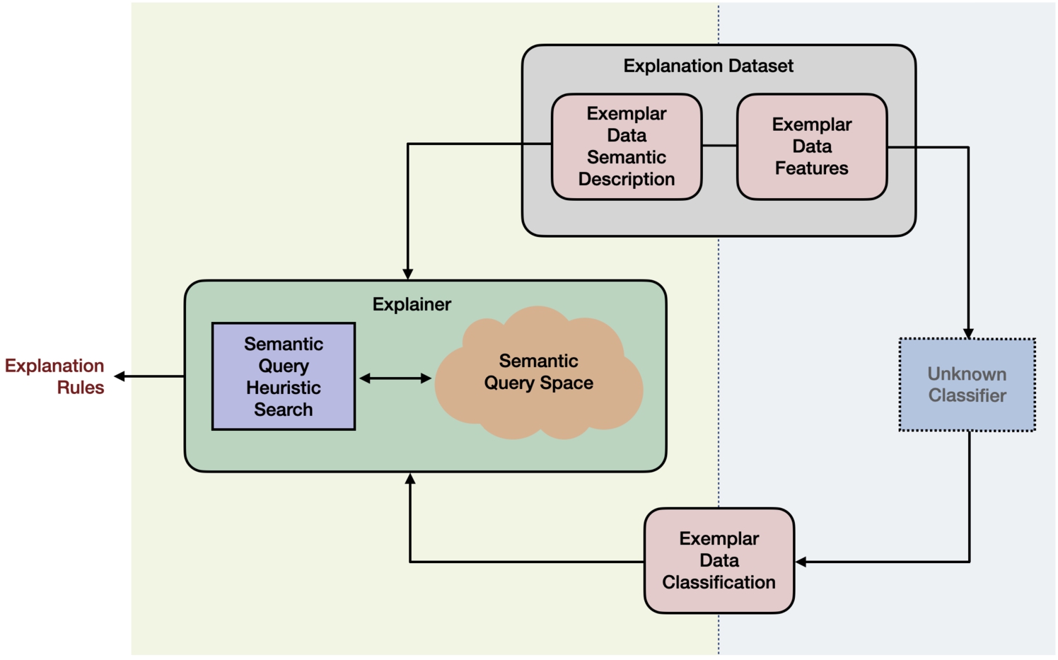
Explanation of opaque machine learning classifiers is based on a dataset that we call Explanation Dataset (see Fig. 1), containing exemplar patterns, that are actually characteristic examples from the set of elements that the unknown classifier takes as input. Machine learning classifiers usually take as input element features (like the cough audio signal mentioned in the motivating example). The explanation dataset additionally contains a semantic description of the exemplars in terms that are understandable by humans (like “dry cough” mentioned in the motivating example). Taking the output of the unknown classifier (the classification class) for all the exemplars, we construct the Exemplar Data Classification information (see Fig. 1) thus we know the exact set of exemplars that are classified by the unknown classifier to a specific class (like the “seek medical advice” class mentioned in the motivating example). Using the knowledge represented in the Exemplar Data Semantic Description (see Fig. 1), we define the following reverse semantic query answering problem: “given a set of exemplars and their semantic description find intuitive and understandable semantic queries that have as certain answers exactly this set out of all the exemplars of the explanation dataset”. The specific problem is interesting, with certain difficulties and computationally very demanding [3,11,19,20,59]. Here, by extending a method presented in [48] we present an Explainer (see Fig. 1) that tries to solve this problem, following a Semantic Query Heuristic Search method, that searches in the Semantic Query Space (the set containing all queries that have non-empty certain answer set) for queries that are solutions to the above problem.
Fig. 1.
A framework for explaining opaque machine learning classifiers.
Introductory definitions and interesting theoretical results concerning the above approach are presented in [48]. Here, we reproduce some of them and introduce others, in order to develop the necessary framework for presenting the proposed method.
A defining aspect is that the rule explanations are provided in terms of a specific vocabulary. To do this in practice, we require a set of items (exemplar data) which can: a) be fed to a black-box classifier and b) have a semantic description using the desired terminology. As mentioned before, here we consider that: a) the exemplar data has for its items all the information that the unknown classifier needs in order to classify them (the necessary features), and b) the semantic data descriptions are expressed as Description Logics knowledge bases (see Fig. 1).
Definition 1
Definition 1([19]).
Let
Intuitively, an explanation dataset contains a set of exemplar data (i.e. characteristic items in
Definition 2
Definition 2([19]).
Let
Note that in the above, the argument of
Explanation rules describe sufficient conditions (the body of the rule) for an item to be classified in the class indicated at the head of the rule by the classifier under investigation. The correctness of a rule indicates that the rule covers every
Example 1.
Suppose we have the problem described in the motivating example of Section 3.1 with black-box classifiers predicting whether a person should seek medical advice based on audios of their cough, and that we are creating an explanation dataset in order to explain the respective classifiers. The vocabulary used should be designed so that it will produce meaningful explanations to the end-user, which in our case would probably be a doctor or another professional of the medical domain. In this case, it should contain concepts for the different medical terms like the findings (cough, sore throat, etc.), and according to the definition of the explanation dataset, the class categories (seek medical advice, or not) and the concept
As mentioned in Section 2, a SAV query is an expression of the form
Definition 3
Definition 3([19]).
Let
This query reverse engineering problem follows the Query by Example paradigm or QbE. This term refers to reverse engineering queries that contain some positive examples in their answer set but not any negative examples and is widely used in the related literature [7,17,32,36,51,56,85]. We give a short formal definition of QbE adapted from [56].
Definition 4
Definition 4(Query by Example).
Given a DL knowledge base
In our case,
The relationship between the properties of explanation rules and the respective queries allows us to detect and compute correct rules based on the certain answers of the respective explanation rule queries, as shown in Theorem 1.
Theorem 1
Theorem 1([19]).
Let
Proof.
Let
Because by definition C does not appear anywhere in
By definition of a certain answer,
Assume that ρ is correct and let
For the inverse, assume that
Theorem 1 shows a useful property of the certain answers of the explanation rule query of a correct rule (
Example 2.
Continuing Example 1, we can create the explanation rule queries of the respective explanation rules of the example as follows:
For the above queries we can retrieve their certain answers over our knowledge base
With respect to the classifier F of Example 1, for which
The explanation framework described in this section provides the necessary expressivity to formulate accurate rules, using a desired terminology, even for complex problems [19]. However, some limitations of the framework, like only working with correct rules, can be a significant drawback for explanation methods built on top of that. An explanation rule query might not be correct due to the existence of individuals in the set of certain answers which are not in the pos-set. By viewing these individuals as exceptions to a rule, we are able to provide as an explanation a rule that is not correct, along with the exceptions which would make it correct if they were omitted from the explanation dataset; the exceptions could provide useful information to an end-user about the classifier under investigation. Thus, we extend the existing framework by introducing correct explanation rules with exceptions, as follows:
Definition 5.
Let
Since we allow exceptions to explanation rules, it is useful to define a measure of precision of the corresponding explanation rule queries as
Obviously, if the precision of a rule query is 1, then it represents a correct rule, otherwise it is correct with exceptions. Furthermore, we can use the Jaccard similarity between the set of certain answers of the explanation rule query and the pos-set, as a generic measure which combines
Example 3.
The rules
Table 3
Metrics and exceptions of the example explanation rules and the respective explanation rule queries
| Rule | Query | Recall | Precision | Degree | Exceptions ( |
| 1.0 | 1.0 | 1.0 | {} | ||
| 0.67 | 1.0 | 0.67 | {} | ||
| 1.0 | 0.75 | 0.75 | {p1} | ||
| 0.33 | 0.5 | 0.25 | {p2} |
It can often be useful to present a set of rules to the end user instead of a single one. This could be, for example, because the pos-set cannot be captured by a single correct rule but only by a set of correct rules. This is a strategy commonly employed by other rule based systems such as those we employed in Section 5 to compare our algorithms to, namely RuleMatrix [53] and Skope-Rules [80]. The metrics already defined for a single query can be expanded to a set of queries
As we have previously mentioned, we do not have any formal guarantees that the semantics expressed in the explanations extracted by the reverse engineering process are linked to the ones used by the classifier. In [63] the author proposes the term “summary of predictions” for approaches such as ours, that are independent of the classifier features, and the explanations are produced by summarizing the predictions of the classifier. We nevertheless use the term explanation to be consistent with the existing literature. The measures we defined in this section provide some confidence about the existence of a link between the semantics of the classifier and those of the explanations. Assuming that the explanations produced are of high quality (high precision, low recall, short in length) and that the explanation dataset is constructed in a way that takes into account possible biases, it is reasonable to assume that there is at least some correlation between the semantics that the explanation presents with those that the classifier is using.
Unfortunately, as the semantic descriptions become richer, it is more likely that a query that perfectly separates the positive and negative individuals exists since the space of queries that can be expressed using the vocabulary of the descriptions becomes larger. This could lead to rules with high precision (and possibly high degree) that do not hold for new examples which could be perceived as a form of overfitting. This resembles the curse of dimensionality of machine learning, where the plethora of features leads to overfitting models when there is a lack of sufficient data. It would be helpful to have some statistical measures after the reverse engineering process that express how likely it is that the query(ies) perform well by coincidence, rather than due to a link between the semantics expressed in the explanation dataset and the ones used by the classifier. Computing such measures is far from trivial due to the complex structure of the Query Space [19]. In this work, we employ some alternatives in our experiments. Namely, using a holdout set in order to check how well the rules produced generalize (Mushrooms experiment, Section 5.1), and employing other XAI methods to cross-reference the explanations produced (Visual Genome experiment, Section 5.3). We consider a thorough examination of such methods to be out of the scope of this work.
4.Computation of explanations
From Section 3, we understand that the problem that we try to solve is closely related to the query reverse engineering problem, since we need to compute queries given a set of individuals. However, since in most cases there is not a single query that fits our needs (have as certain answers the pos-set of the classifier), we need to find (out of all the semantic queries that have a specific certain answer set) a set of queries that accurately describe the classifier under investigation. Therefore, the problem can also be seen as a heuristic search problem. The duality of rules and queries within our framework, reduces the search of correct rules (with exceptions) to the search of queries that contain elements of the pos-set in their certain answers. Reverse engineering queries for subsets of
– The subsets of
– The Query Space i.e. the set containing all queries that have non-empty certain answer set (
– For any subset I of
– Computing the certain answers of arbitrary queries can be exponentially slow, so it is computationally prohibitive to evaluate each query under consideration while exploring the query space.
– In this paper, we only consider knowledge bases of which the TBox can be eliminated (such as RL [38]; see also the last paragraph of this section). This enables us to create finite queries that contain all the necessary conjuncts to fully describe each individual. We are then able to merge those queries to create descriptions of successively larger subsets of
– We do not directly explore the subsets of
– We are not concerned with the entire set of queries with non-empty sets of certain answers, but only with queries which have specific characteristics in order to be used as explanations. Specifically, the queries have to be short in length, with no redundant conjuncts, have as certain answers elements of the pos-set of the class under investigation, and as few others as possible.
– One of the proposed algorithms guarantees that given a set I, if a query q exists s.t.
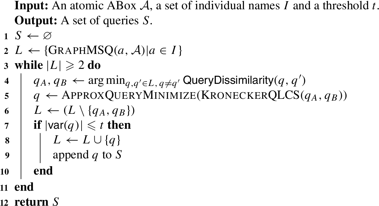
In the following we describe the proposed algorithms for computing explanations. The core algorithm, which is outlined as Alg. 1 and we call KGrules-H, takes as input an atomic ABox
Algorithm 1:
KGRules-H
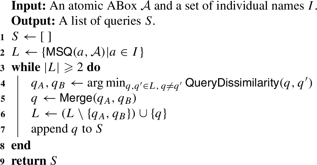
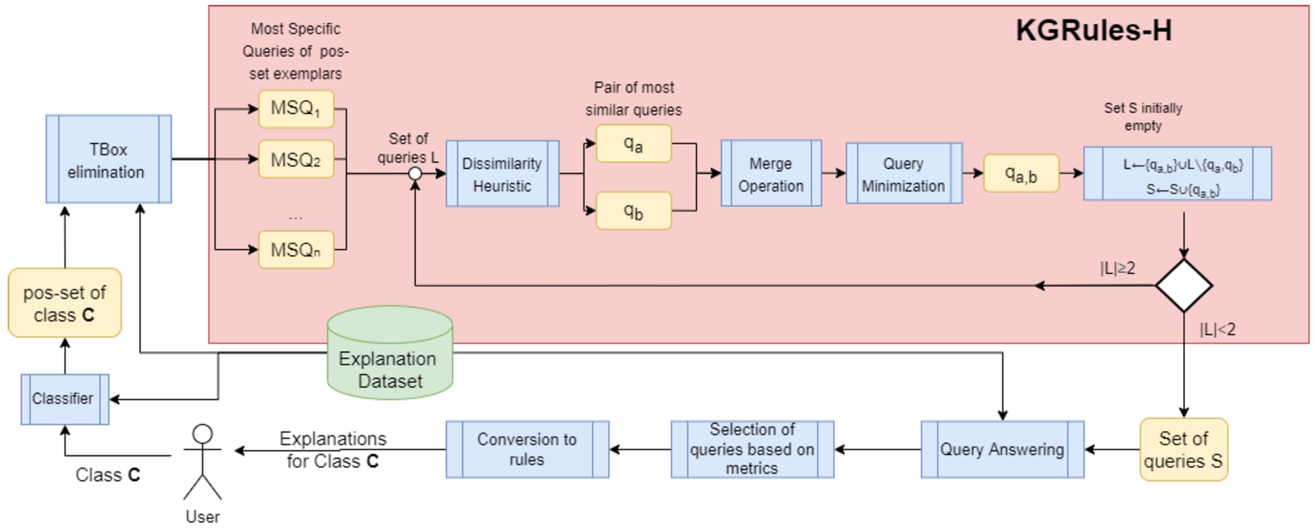
Fig. 2.
Visualization of how KGrules-H is integrated into our framework.
The algorithm starts by initializing an empty list of queries S, and by creating an initial description for each individual in I in the form of a most specific query (MSQ). A detailed definition of a MSQ is given in Section 4.1; intuitively, an MSQ of an individual a for an ABox
If the queries in S have subsets of I as their certain answers, given that we have assumed that I is the pos-set of a classifier for some class C, the queries can be treated as candidate explanation rule queries for C. In this case, the queries can be interpreted as explanation rule queries, converted to the respective explanation rules, and presented as explanations. In general, however, there is no guarantee that the certain answers of a merged query will be a subset of I. In this case, which is the typical case, the computed explanation rules will be rules with exceptions. The queries produced will differ with respect to the metrics introduced in Section 3. Specifically, the queries produced early on, which are the result of few merges are expected to have low recall but high precision, with the inverse holding for queries produced in the later iterations. The importance placed on each metric can be different for each end user, therefore there is no single best query produced by Alg. 1. Instead, metrics for each query should be produced and presented to the end user to let them rank the explanations according to their preferences. This is the methodology we have employed in Section 5. For each experiment conducted we present a selection of queries, each performing better for a different metric.
In Section 4.3 we prove some optimality results for one of the merging methods, the query least common subsumer (QLCS). In particular, if there is a correct explanation rule (without exceptions), then we are guaranteed to find the corresponding explanation rule query, using the QLCS. This optimality property does not hold for the Greedy Matching operation defined in Section 4.3.2, nor for Alg. 3.
As mentioned above, Alg. 1 works on the assumption that all available knowledge about the relevant individuals I is encoded in a (finite) atomic ABox
4.1.Most specific queries
As mentioned above, intuitively, a most specific query (MSQ) of an individual a for an atomic ABox
Following the subsumption properties, MSQs are unique up to syntactical equivalence. In Alg. 1 it is assumed that
Theorem 2.
Let
Proof.
Let
Since f exists, we can construct for q the match
Since
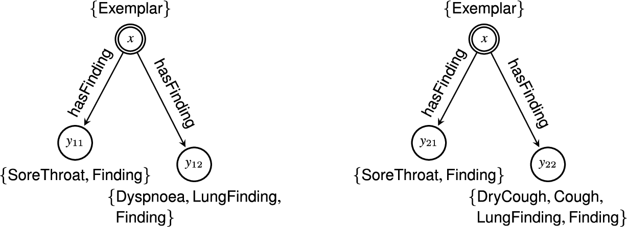
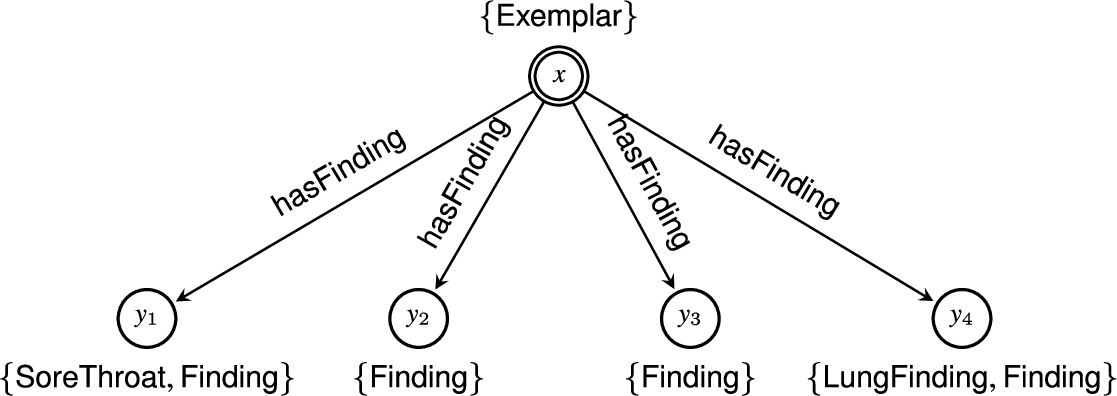
Example 4.
Continuing the previous examples, Fig. 3 shows the graphs of the MSQs of
Fig. 3.
The MSQs of
For use with Alg. 1, we denote a call to a concrete function implementing the above described approach for obtaining
4.2.Query dissimilarity
At each iteration, Alg. 1 selects two queries to merge in order to produce a more general description covering both queries. To make the selection, we use a heuristic which is meant to express how dissimilar two queries are, so that at each iteration the two most similar queries are selected and merged, with the purpose of generating an as least generic as possible more general description. Given two queries
The intuition behind the above dissimilarity measure is that the graphs of queries which are dissimilar consist of nodes with dissimilar labels connected in dissimilar ways. Intuitively, we expect such queries to have dissimilar sets of certain answers, although there is no guarantee that this will always be the case. In order to have a heuristic that can be computed efficiently, we do not examine complex ways in which the nodes may be interconnected, but only examine the local structure of the nodes by comparing their indegrees and outdegrees. The way in which we compare the nodes of two query graphs is optimistic; we compare each node with its best possible counterpart —the node of the other graph which it is the most similar to. Note that
Example 5.
Let
Using an efficient representation of the queries, it is easy to see that
4.3.Query merging
The next step in Alg. 1 is the merging of the two most similar queries that have been selected. In particular, given a query
4.3.1.Query least common subsumer
Our first approach for merging queries is using the query least common subsumer (QLCS). In the next few paragraphs we will present how to construct such a query from two SAV queries which will make apparent that the QLCS of two SAV queries always exists. As mentioned in Section 2, a QLCS is a most specific generalization of two queries. By choosing to use
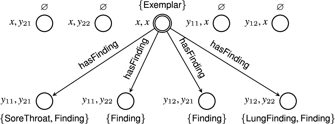
To compute a QLCS we use an extension of the Kronecker product of graphs to labeled graphs. Given two labeled graphs
Fig. 4.
The Kronecker product of the MSQs of
As with the Kronecker product of unlabeled graphs, for any graph H, we have that
For use with Alg. 1, we denote a call to the concrete function implementing that approach for computing
Example 7.
Fig. 5 shows the QLCS of the MSQs of Example 4, extracted from the Kronecker product of Example 6. It is obvious that the nodes with label
Fig. 5.
The QLCS of the MSQs of
Removing the redundant parts of a query is essential not only for reducing the running time of the algorithm. Since these queries are intended to be shown to humans as explanations, ensuring that they are compact is imperative to improve comprehensibility. As mentioned in Section 2, the operation that compacts a query by creating a syntactically equivalent query by removing all its redundant parts is condensation. However, condensing a query is coNP-complete [27]. For this reason, we utilize Alg. 2, an approximation algorithm which removes redundant conjuncts and variables without a guarantee of producing a fully condensed query.
Algorithm 2:
ApproxQueryMinimize
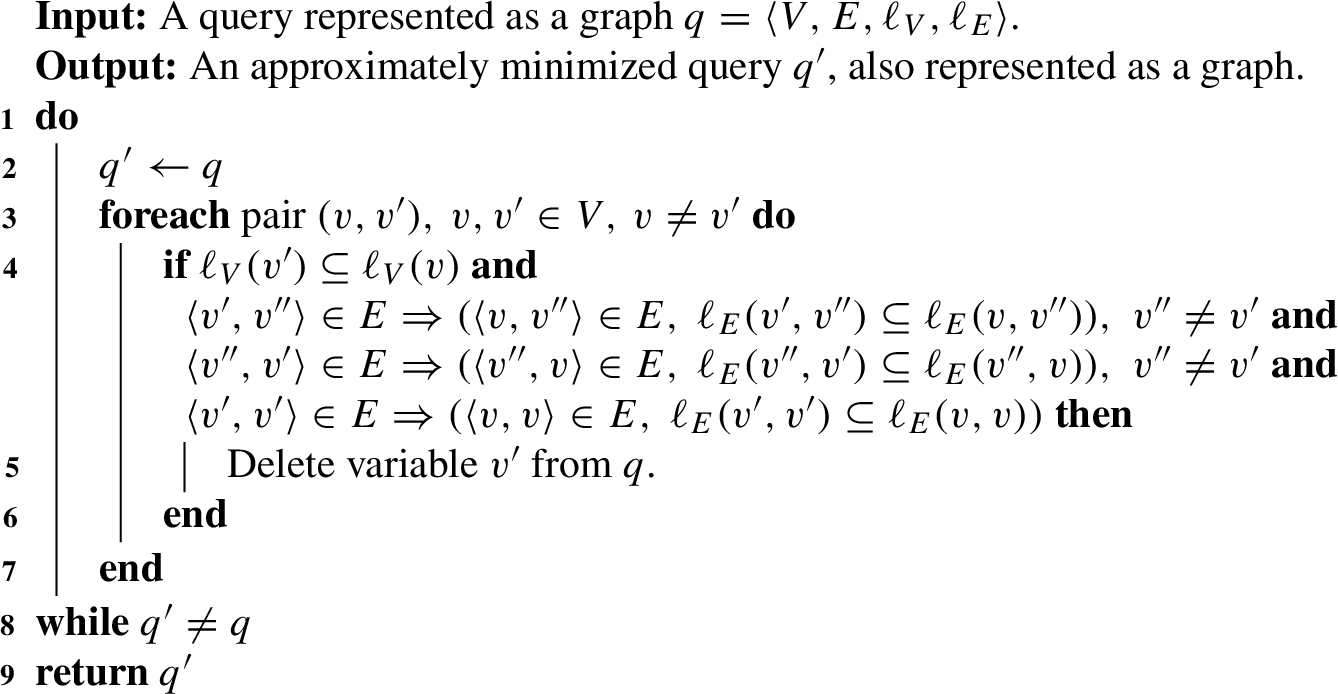
Alg. 2 iterates through the variables of the input query, and checks if deleting one of them is equivalent to unifying it with another one. In particular, at each iteration of the main loop, the algorithm attempts to find a variable suitable for deletion. If none is found, the loop terminates. The inner loop iterates through all pairs of variables. At each iteration, variable
Example 8.
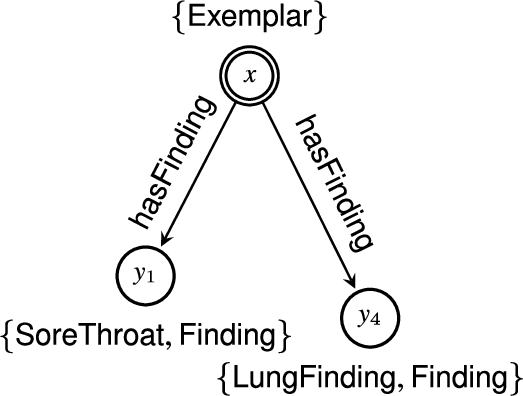
We can showcase an example of Alg. 2 detecting an extraneous variable in the QLCS of
The main loop of Alg. 2 is executed at most
Given the above, our first practical implementation of Alg. 1, uses
Regardless of the approximate query minimization described above, even if full query condensation could be performed, there is no guarantee that condensing the queries computed by Alg. 1 using QLCS as the merge operation, have meaningfully smaller condensations. This led us to two different approaches for further dealing with the rapidly growing queries QLCS produces.
The simplest approach to address this problem is to reject any queries produced by
Algorithm 3:
KGrules-HT
Alg. 3 is the same as Alg. 1 except that q is not added to L and S unless its variable count is less than or equal to an input threshold, t. This simple change reduces the complexity of the algorithm to polynomial in terms of
If we let
Our second approach to overcome the problem posed by the rapidly growing size of the queries produced by QLCS was to consider a different merge operation, which is described in the following section.
4.3.2.Greedy matching
As already mentioned, the above described procedure for merging queries by computing a QLCS, often introduces too many variables that Alg. 2 can’t minimize effectively. A QLCS of
One such method, is finding a common subquery, i.e. finding the common conjuncts of two queries
Example 9.
Continuing the previous examples, we will find common subqueries of the MSQs of
Finding the maximum common subquery belongs to a larger family of problems of finding maximal common substructures in graphs, such as the mapping problem for processors [8], structural resemblance in proteins [29] and the maximal common substructure match (MCSSM) [79]. Our problem can be expressed as a weighted version of most of these problems, since they only seek to maximize the number of nodes in the common substructure, which, in our case, corresponds to the number of variables in the resulting subquery. Since we want to maximize the number of common conjuncts, we could assign weights to variable matchings (y corresponds to z) due to concept conjuncts, and to pairs of variable matchings (y corresponds to z and
Algorithm 4:
GreedyCommonConjuncts
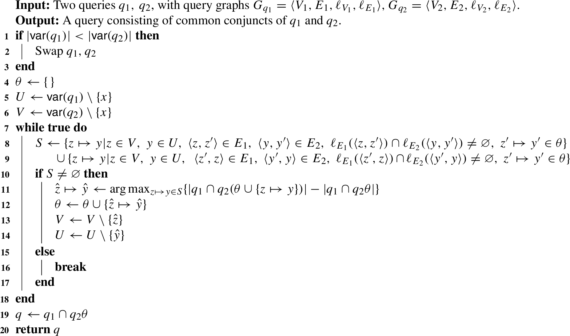
Alg. 4 initializes an empty variable renaming θ. V and U contain the variables that have not been matched yet. At each iteration of the main loop, the algorithm attempts to match one of the variables of
An efficient implementation of Alg. 4 will use a max-priority queue to select at each iteration the match that adds the largest number of conjuncts to the induced query. The priority queue should contain an element for each pair of variables that can be matched, with the priority of the element being either 0 if the pair is not in S, and otherwise equal to the number of conjuncts it would add to the query. At each iteration some priorities may need to be updated. The time complexity of priority queues varies depending on their implementation. Implementations such as Strict Fibonacci Heaps have lower time complexity but perform worse in practice than simpler implementations with higher time complexities such as Binary Heaps. A Strict Fibonacci Heap implementation would have a time complexity of
5.Experiments
We evaluated the proposed algorithms and framework by generating explanations for various classifiers, computing the metrics presented in Section 3, comparing with other rule-based approaches where possible, and discussing the quality and usefulness of the results.11 Specifically, we explored four use-cases: a) we are given a tabular dataset which serves as both the features of the classifier and the explanation dataset, b) we are given raw data along with curated semantic descriptions (ABox) but without a TBox, c) we are given curated semantic descriptions, along with a TBox, and d) we are only given raw data, so semantic descriptions need to be constructed automatically. The first use-case facilitated comparison of the proposed KGRules-H algorithm with other rule-based XAI approaches from literature, the second and third use-cases were more suitable for validating the usefulness of the proposed framework in its intended setting, while the fourth explored how KGRules-H could be utilized in a scenario in which semantic data descriptions are not available. For the first use-case we experimented on the Mushroom22 dataset which involves only categorical features. For the second use-case we used the CLEVR-Hans3 dataset [68] which consists of images of 3D geometric shapes in addition to rich metadata which we use as semantic data descriptions. For the third we constructed an explanation dataset from a subset of the Visual Genome [39] to explain a classifier trained on Places365 [83] for scene classification, while for the fourth we used MNIST [43] which contains images of handwritten digits, and no metadata.
The components needed for each experiment, were: a) a black-box classifier for which we provide rule-based explanations, b) an explanation dataset with semantic descriptions of exemplar data using the appropriate terminology and c) reasoning capabilities for semantic query answering, in order to evaluate the generated rules. As classifiers we chose widely used neural networks, which are provided as default models in most deep learning frameworks.
For constructing explanation datasets in practice, we identified two general approaches: a) the curated approach, and b) the automated information extraction approach. For the manual curated approach, the semantic descriptions of exemplar data were provided. In an ideal scenario, curated explanation datasets are created by domain experts, providing semantic descriptions which are meaningful for the task, and by using the appropriate terminology, lead to meaningful rules as explanations. In our experiments, we simulated such a manually curated dataset by using Visual Genome, which provides semantic descriptions for each image present in the dataset, using terminology linked to WordNet [52]. Of course, using human labor for the creation of explanation datasets in real-world applications would be expensive, thus we also experimented with automatically generating semantic descriptions for exemplar data. Specifically, for the automated information extraction approach we used domain specific, robust, feature extraction techniques and then provided semantic descriptions in terms of the extracted features. In these experiments, we automatically generated semantic descriptions for images in MNIST, by using ridge detection, and then describing each image as a set of intersecting lines.
For acquiring certain answers of semantic queries, which requires reasoning, we set up repositories on GraphDB.33 For the case of the Mushrooms dataset we used the certain answers to measure fidelity, number of rules and average rule length and compared our approach with RuleMatrix [53] which implements scalable bayesian rule lists [80], Skope-Rules44 and the closely related KGrules [19]. For CLEVR-Hans3, we mainly used the certain answers to explore whether our explainability framework can detect the foreknown bias of the classifier, while for Visual Genome we attempt to discover biases, by observing the best generated rule-queries with respect to precision, recall, and degree as defined in Section 3. Finally, for MNIST we observed quality and usability related properties of generated rule queries and their exceptions.
5.1.Mushrooms
The purpose of the Mushroom experiment was to compare our results with other rule-based approaches from the literature. Since other approaches mostly provide explanation rules in terms of the feature space, the explanation dataset was created containing only this information. We should note that this was only done for comparison’s sake, and is not the intended use-case for the proposed framework, in which there would exist semantic descriptions which cannot be necessarily represented in tabular form, and possibly a TBox.
5.1.1.Explanation dataset
The Mushroom dataset contains 8124 rows, each with 22 categorical features of 2 to 9 possible values. We randomly chose subsets of up to 4000 rows to serve as the exemplars of explanation datasets. The vocabulary
5.1.2.Setting
For this set of experiments, we used a simple multi-layer perceptron with one hidden layer as the black-box classifier. The classifier achieved
We split the dataset into four parts: 1) a training set, used to train the classifier, 2) a test set, used to evaluate the classifier, 3) an explanation-train set, used to generate explanation rules, and 4) an explanation-test set, used to evaluate the generated explanation rules. When running KGrules-H and KGrules, the explanation dataset was constructed from the explanation-train set. We experimented by changing the size of this dataset, from 100 to 4000 rows, and observed the effect it had on the explanation rules. On the explanation-test set, we measured the fidelity of the generated rules which is defined as the proportion of items for which classifier and explainer agree. We also measured the number of generated rules and average rule length. We used the proposed KGrules-H algorithm to generate explanations, and we also generated rules (on the same data and classifier) with RuleMatrix, Skope-rules and the closely related KGrules.
To compare with the other methods, which return a set of rules at their output, in this experiment we only considered correct rules we generated. To choose which rules to consider (what would be shown to a user), from the set of all correct rule-queries generated, we greedily chose queries starting with the one that had the highest count of certain answers on the explanation-train set, and then iteratively adding queries that provided the highest count of certain answers, not provided by any of the previously chosen queries. This is not necessarily the optimal strategy of rule selection for showing to a user (it never considers rules with exceptions), and we plan to explore alternatives in future work.
Finally, for all methods except for the related KGrules we measured running-time using same runtime on Google Colab,55 by using the “%%timeit”66 magic command with default parameters. KGrules was not compatible with this benchmarking test, since it is implemented in Java as opposed to Python which is the implementation language provided for the other methods. In addition, KGrules implements an exhaustive exponential algorithm, so it is expected to be much slower than all other methods.
5.1.3.Results
The results of the comparative study are shown in Table 4. A first observation is that for small explanation datasets, the proposed approach did not perform as well as the other methods regarding fidelity, while for large ones it even outperformed them. This could be because for small explanation datasets, when the exemplars are chosen randomly, there are not enough individuals, and variety in the MSQs of these individuals, for the algorithm to generalize by merging their MSQs. This is hinted also from the average rule length, which is longer for both KGrules-H and KGrules for explanation dataset sizes 100 and 200, which indicates less general queries. Conversely, for explanation datasets of 600 exemplars and larger, the proposed approach performs similarly, in terms of fidelity, with related methods. Regarding running time, KGrules-H is the fastest except for the case of the largest explanation dataset, for which Skope-rules is faster. However, in this case Skope-rules’s performance suffers with respect to fidelity, whereas RuleMatrix and KGrules-H achieve perfect results. Furthermore, our proposed approach seems to generate longer rules than all other methods which on the one hand means that they are more informative, though on the other hand they are potentially less understandable by a user. This highlights the disadvantages constructing queries using the MSQs as a starting point. This was validated upon closer investigation, where we saw that the rules generated from the small explanation datasets were more specific than needed, as the low value of fidelity was due only to false negatives, and there were no false positives. Detecting redundant conjuncts might be done more efficiently for rules concerning tabular data, but for general rules, on which our approach is based, this task is very computationally demanding.
Table 4
Performance on the mushroom dataset
| Size | Method | Fidelity | Nr. of rules | Avg. length | Time (seconds) |
| 100 | KGrules-H | 92.70% | 4 | 14 | 0.15 |
| KGrules | 97.56% | 11 | 5 | - | |
| RuleMatrix | 94.53% | 3 | 2 | 3.65 | |
| Skope-rules | 97.01% | 3 | 2 | 1.29 | |
| 200 | KGrules-H | 93.40% | 8 | 14 | 0.18 |
| KGrules | 98.37% | 11 | 5 | - | |
| RuleMatrix | 97.78% | 4 | 2 | 3.65 | |
| Skope-rules | 98.49% | 4 | 2 | 1.47 | |
| 600 | KGrules-H | 99.60% | 10 | 13.3 | 0.61 |
| KGrules | 99.41% | 13 | 4 | - | |
| RuleMatrix | 99.43% | 6 | 1 | 7.69 | |
| Skope-rules | 98.52% | 4 | 2 | 1.58 | |
| 1000 | KGrules-H | 100% | 9 | 14.2 | 1.67 |
| KGrules | 99.58% | 14 | 6.57 | - | |
| RuleMatrix | 99.90% | 6 | 1.33 | 11.1 | |
| Skope-rules | 98.50% | 4 | 2.25 | 2.95 | |
| 4000 | KGrules-H | 100% | 10 | 14.2 | 34.30 |
| KGrules | 99.72% | 16 | 5.81 | - | |
| RuleMatrix | 100% | 7 | 1.43 | 43.00 | |
| Skope-rules | 96.85% | 2 | 2 | 3.01 |
5.2.CLEVR-Hans3
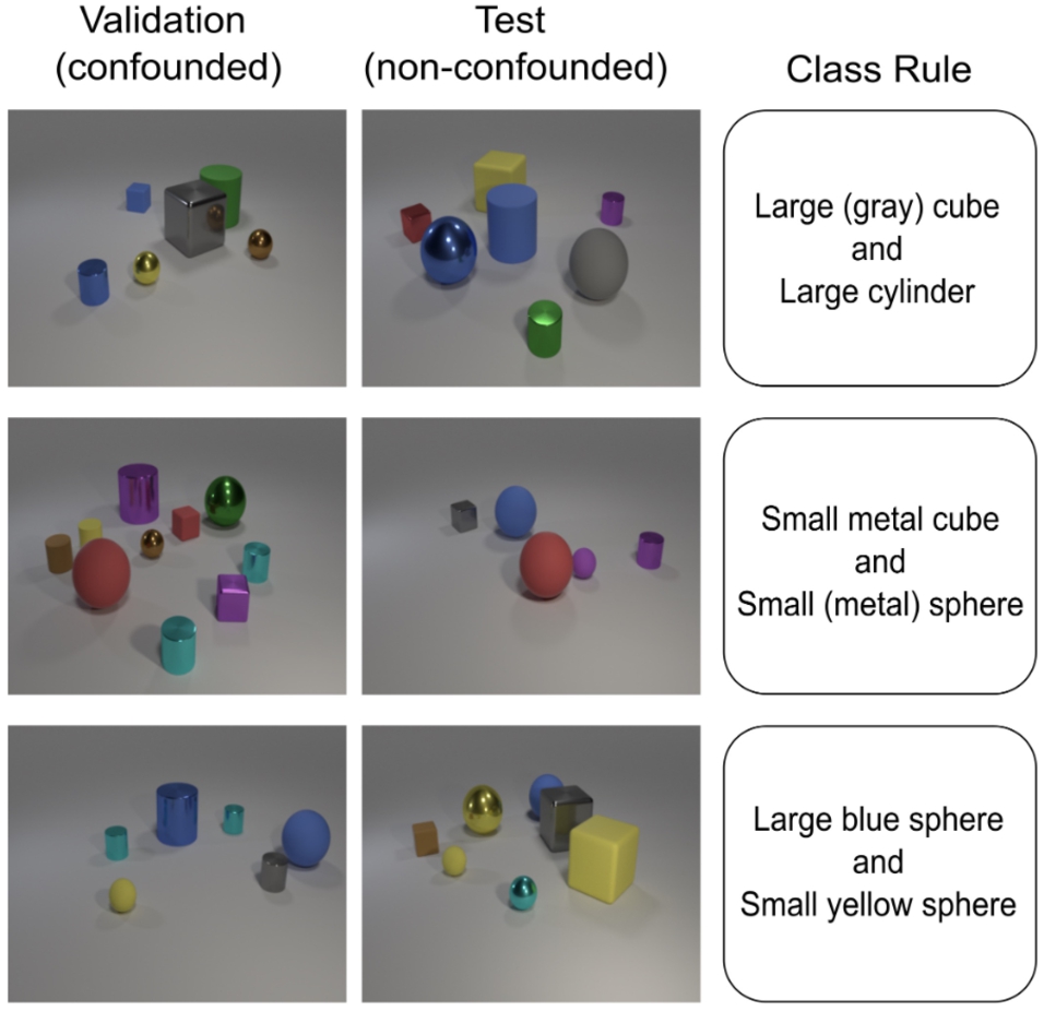
The second set of experiments involved CLEVR-Hans3 [68], which is an image classification dataset designed to evaluate algorithms that detect and fix biases of classifiers. It consists of CLEVR [35] images divided into three classes, of which two are confounded. The membership of an image to a class is based on combinations of the attributes of the objects depicted. Thus, within the dataset, consisting of train, validation, and test splits, all train, and validation images of confounded classes will be confounded with a specific attribute. The rules that the classes follow are the following, with the confounding factors in parentheses: (i) Large (Gray) Cube and Large Cylinder, (ii) Small Metal Cube and Small (Metal) Sphere, (iii) Large Blue Sphere and Small Yellow Sphere (Fig. 7). This dataset provides sufficient and reliable information to create an explanation dataset, while the given train-test split contains intentional biases, which was ideal as a grounds for experimentation, as we could observe the extent to which the proposed explanation rules can detect them.
5.2.1.Explanation dataset
Fig. 7.
Image samples of the three classes of CLEVR-Hans3 along with the class rules and the confounding factors in parentheses.
We created an explanation dataset
5.2.2.Setting
For the experiments on CLEVR-Hans3 we used the same ResNet34 [33] classifier and training procedure as those used by the creators of the dataset in [68]. The performance of the classifier is shown in Table 5 and so is the confusion matrix which summarizes the predictions of the classifier indicating the differences between the actual and the predicted classes of the test samples. As expected, the classifier has lower values on some metrics regarding the first two classes, and this is attributed to the confounding factors and not the quality of the classifier, since it achieved
Table 5
Performance of the ResNet34 model on CLEVR-Hans3
| True label | Test set metrics | Confusion matrix | ||||
| Precision | Recall | F1-score | Class 1 | Class 2 | Class 3 | |
| Class 1 | 0.94 | 0.16 | 0.27 | 118 | 511 | 121 |
| Class 2 | 0.59 | 0.98 | 0.54 | 5 | 736 | 9 |
| Class 3 | 0.85 | 1.00 | 0.92 | 2 | 0 | 748 |
5.2.3.Results
The explanation rules generated for the ResNet34 classifier using KGrules-H and QLCS as the merge operation, as outlined in Section 4.3.1, are shown in Table 6, where we show the rule, the value of each metric and the numbers of positive individuals. The term positive individuals refers to the certain answers of the respective explanation rule query that are also elements of the pos-set (they are classified in the respective class).
In our representation of explanation rule queries in Tables 6, 7 we have omitted the answer variable x, along with all conjuncts of the form x contains y and conjuncts of the form
The algorithm found a correct rule (
It is interesting to note that the rule query with recall = 1 produced for class 1 contained a Large Cube but not a Large Cylinder, which is also in the description of the class. This shows that in the training process the classifier learned to pay more attention to the presence of cubes rather than the presence of cylinders. The elements of the highest recall correct rule that differ from the true description of class 1 can be a great starting point for a closer inspection of the classifier. We expected the presence of a Gray Cube from the confounding factor introduced in the training and validation sets, but in a real world scenario similar insights can be reached by inspecting the queries. In our case, we further inquired the role that the Gray Cube and the Large Metal Object play in the correct rule by removing either of them from the query and examining its behavior. In Table 7 we can see that the gray color was essential for the correct rule while the Large Metal Object was not, and in fact its removal improved the rule and returned almost the entire class.
Another result that piqued our attention was the highest degree explanation for class 3 which is the actual rule that describes this class. This explanation was not a correct rule, since it had two exceptions, which we can also see in the confusion matrix of the classifier and we were interested to examine what sets these two individuals apart. We found that both of these individuals are answers to the query “y1 is Large, Gray, Cube”. This showed us once again the great effect the confounding factor of class 1 had on the classifier.
Our overall results show that the classifier tended to emphasize low level information such as color and shape and ignored higher level information such as texture and the combined presence of multiple objects. This was the reason why the confounding factor of class 1 had an important effect to the way images were classified, while the confounding factor of class 2 seemed to have had a much smaller one. Furthermore, the added bias made the classifier reject class 1 images, which however had to be classified to one of the other two classes (no class was not an option). Therefore one of the other classes had to be “polluted” by samples which were not confidently classified to a class. This motivates us to expand the framework in the future to work with more informative sets than the pos-set, such as elements which were classified with high confidence, and false and true, negatives and positives
Table 6
Optimal explanations with regard to the three metrics on CLEVR-Hans3
| Metric | Explanation rules | Precision | Recall | Degree | Positives |
| Class 1 | |||||
| Best precision | y1 is Large, Cube, Gray. | 1.00 | 0.66 | 0.66 | 83 |
| y2 is Large, Cylinder. | |||||
| y3 is Large, Metal. | |||||
| Best recall | y1 is Large, Cube. | 0.09 | 1.00 | 0.09 | 125 |
| Best degree | y1 is Large, Cube, Gray. | 1.00 | 0.66 | 0.66 | 83 |
| y2 is Large, Cylinder. | |||||
| y3 is Large, Metal. | |||||
| Class 2 | |||||
| Best precision | y1 is Small, Sphere. | 1.00 | 0.09 | 0.09 | 116 |
| y2 is Large, Rubber. | |||||
| y3 is Small, Metal, Cube. | |||||
| y4 is Small, Brown. | |||||
| y5 is Small, Rubber, Cylinder. | |||||
| Best recall | y1 is Cube. | 0.63 | 1.00 | 0.63 | 1247 |
| Best degree | y1 is Metal, Cube. | 0.78 | 0.8 | 0.65 | 1005 |
| y2 is Small, Metal. | |||||
| Class 3 | |||||
| Best precision | y1 is Metal, Blue. | 1.00 | 0.42 | 0.42 | 365 |
| y2 is Large, Blue, Sphere. | |||||
| y3 is Yellow, Small, Sphere. | |||||
| y4 is Small, Rubber. | |||||
| y5 is Metal, Sphere. | |||||
| Best recall | y1 is Large. | 0.42 | 1.00 | 0.42 | 878 |
| y2 is Sphere. | |||||
| Best degree | y1 is Yellow, Small, Sphere. | 0.99 | 0.85 | 0.85 | 748 |
| y2 is Large, Blue, Sphere. | |||||
Table 7
Two modified versions of the class 1 correct rule produced by removing conjuncts
| Query | Positives | Negatives |
| y1 is Large, Cube. y2 is Large, Cylinder. y3 is Large, Metal. | 108 | 547 |
| y1 is Large, Cube, Gray. y2 is Large, Cylinder. | 93 | 0 |
5.3.Visual genome and places
For the third set of experiments, we produced explanations of an image classifier trained on the Places365 dataset for scene classification. To do this, we constructed an explanation dataset from a subset of the visual genome, which includes a scene-graph for each image. Nodes of scene-graphs represent depicted objects, and edges represent relationships between them, while both edges and nodes are labeled with WordNet synsets. This allows us to encode the provided scene-graphs as an ABox, and to use the hyponym-hypernym hierarchy of WordNet as a TBox.
5.3.1.Explanation dataset
To construct the explanation dataset, we first selected the two most confused classes based on the confusion matrix of the classifier on the Places365 test set. These were “Desert Sand” and “Desert Road”. Then, we acquired the predictions of the classifier on the entirety of the visual genome dataset, and kept as expemplars the images for which the top prediction was one of the aformentioned classes. There were 273 such images. We defined a vocabulary
5.3.2.Setting
As a black-box classifier in this set of experiments we used the ResNet50 classifier77 provided by the official GitHub repository88 for models pretrained on Places365, which classifies images to 365 different classes.99 The top1 error is
5.3.3.Results
The best rule queries for each metric for each of the two classes is shown in Table 8. For simplicity of presentation, we have ommited conjuncts of the form
Table 8
Optimal explanations with regard to the three metrics using the VG explanation dataset
| Metric | Explanation rules | Precision | Recall | Degree | Positives |
| Desert Road | |||||
| Best precision | y1 is field.n.01. | 1.00 | 0.12 | 0.12 | 16 |
| y2 is natural_object.n.01. | |||||
| y3 is giraffe.n.01. | |||||
| y4 is body_part.n.01. | |||||
| y5 is woody_plant.n.01. | |||||
| Best recall | y1 is organism.n.01 | 0.54 | 1.00 | 0.54 | 139 |
| Best degree | y1 is animal.n.01 | 0.72 | 0.84 | 0.64 | 118 |
| Desert Sand | |||||
| Best precision | y1 is instrumentality.n.03 | 1.00 | 0.12 | 0.12 | 16 |
| y2 is road.n.01 | |||||
| y3 is communication.n.02 | |||||
| y4 is sky.n.01 | |||||
| y5 is tree.n.01 | |||||
| Best recall | y1 is physical_entity.n.01 | 0.49 | 1.00 | 0.49 | 134 |
| Best degree | y1 is instrumentality.n.01 | 0.92 | 0.56 | 0.56 | 76 |
| y2 is road.n.01 | |||||
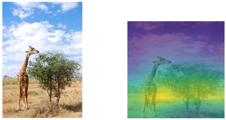
In Fig. 8 we present the saliency maps of three images from Visual Genome classified as “Desert Road” on the left and three classified as “Desert Sand” on the right. The saliency maps support the associations the queries highlighted, namely that images containing animals, especially giraffes, get classified as “Desert Road”, while images with roads and vehicles get classified as “Desert Sand”. Not all images exhibited such strong association. In Fig. 9 the classifier seems to be mostly influenced by the ground which is covered in dry grass. Given that the second highest value in the confusion matrix of this classifier was for the pair “Desert Sand”, “Desert Vegetation” we conjencture that some mistakes were made during the training of this classifier or several images in the training set of the Places365 dataset are mislabeled. The classifier may have been fed images that should be described as “Desert Road” but with the target label being “Desert Sand” and images that should be described as “Desert Vegetation” but with the target label being “Desert Road”. This would explain the weird associations exhibited and the conjuncts appearing in the explanations. The association of giraffes with the label “Desert Road” can be explained with mislabeled images depicting desert vegetation. This is still a wrongful association since giraffes can also populate grasslands such as in the top left image of Fig. 8.
We would like to point out that our method of producing explanations discovered these erroneous associations without asking from the end-user to manually inspect the heatmaps of a large number of images, rather than to read the best performing query for each one of our metrics. We believe that this provides a better user experience since it requires less effort for the initial discovery of suspect associations, which can then be thoroughly tested by examining other explanations such as heatmaps. Our method is also model-agnostic, while methods such as Score-CAM require access to the layers within a convolutional neural network.
Fig. 8.
Images from the visual genome dataset and their saliency maps produced by Score-CAM. Images on the left were classified as “Desert Road” and images on the right as “Desert Sand”.
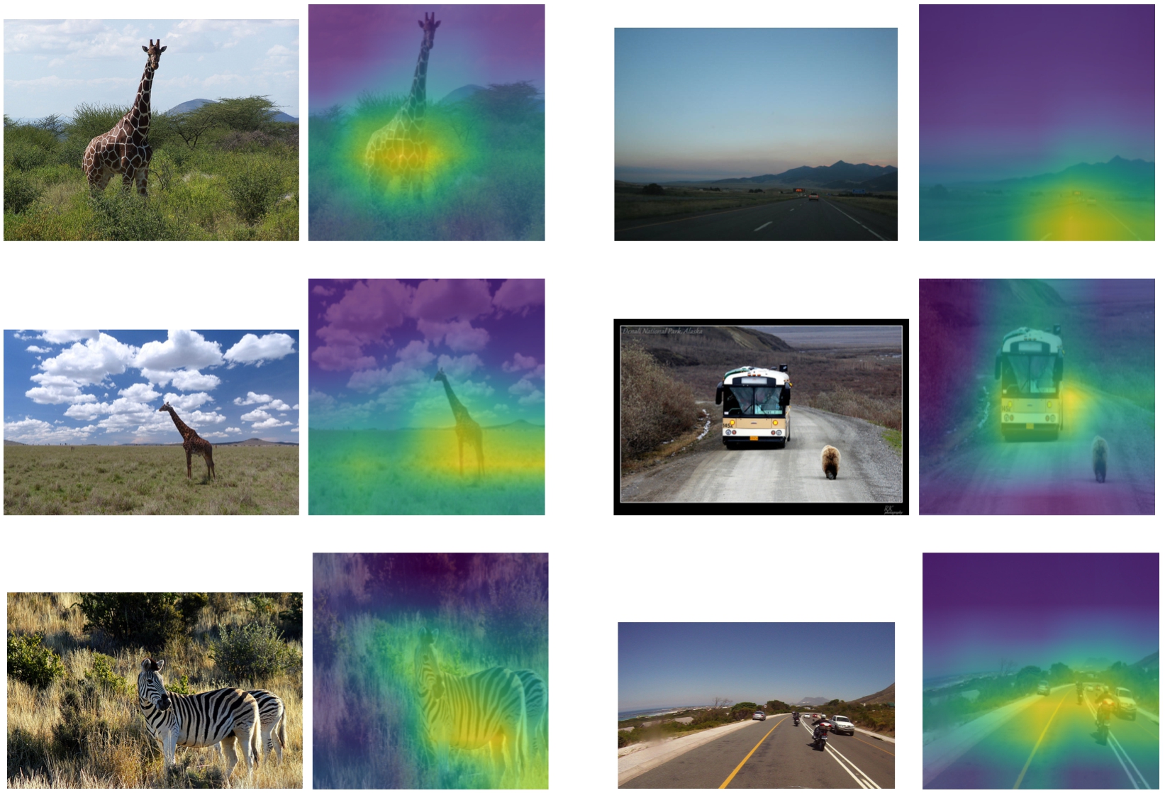
Fig. 9.
An image classified as “Desert Road” exhibiting weaker association to the presence of a giraffe.
5.4.MNIST
For the fourth and final set of experiments we used MNIST, which is a dataset containing grayscale images of handwritten digits [43]. It is a very popular dataset for machine learning research, and even though classification on MNIST is essentially a solved problem, many recent explainability approaches experiment on this dataset (for example [60]). For us, MNIST was ideal for experimenting with automatic explanation dataset generation by using traditional feature extraction from computer vision. An extension to this approach would be using more complex information extraction from images, such as object detection or scene graph generation, for applying the explainability framework to explain generic image classifiers. This however is left for future work.
5.4.1.Explanation dataset
For creating the explanation dataset for MNIST, we manually selected a combination of 250 images from the test set, including both typical and unusual exemplars for each digit. The unusual exemplars were chosen following the mushroom experiment (Section 5.1), in which we saw that small explanation datasets do not facilitate good explanation rules when the exemplars are chosen randomly, so we aimed for variety of semantic descriptions. In addition, the unusual exemplars tended to be misclassified, and we wanted to see how their presence would impact the explanations.
Since there was no semantic information available that could be used to construct an explanation dataset, we automatically extracted descriptions of the images, by using feature extraction methods. Specifically, the images were described as a collection of intersecting lines, varying in angle, length and location within the image. These lines were detected using the technique of ridge detection [50]. The angles of the lines were quantized to 0, 45, 90 or 135 degrees, and the images were split into 3 horizontal (top, middle, bottom) and 3 vertical (left, center, right) zones which define 9 areas (top left, top center,
Fig. 10.
An example of a digit, the results of ridge detection, and the corresponding description.
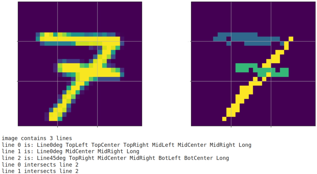
Based on the selected images and the extracted information, we created our explanation dataset
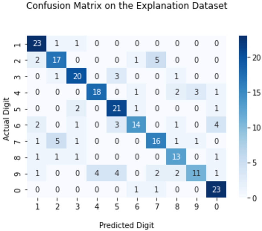
5.4.2.Setting
For MNIST we used the example neural network provided by PyTorch1010 as the classifier to be explained. The classifier achieved 99.8% accuracy on the training set and 99.2% on the test set. On the explanation dataset, the accuracy is 73%, and a confusion matrix for the classifier on the explanation dataset is shown in Fig. 11. The performance of the classifier is poor when compared to the whole test set, due to the fact that we have included several manually selected exemplars, which are unusually drawn, but still valid as digits (based on our own judgement). Similarly to CLEVR-Hans3, we generated explanations for the predictions of the classifier on the exemplars using KGrules-HT (Alg. 3) and KGrules-H (Alg. 1) with Alg. 4 as the merge operation, and loaded the explanation dataset in GraphDB for acquiring certain answers. We also experimented with the QLCS as the merge operation, but the resulting queries mostly contained a large number of variables which could not be effectively minimized, which could be due to the complex connections between variables with a symmetric role.
Fig. 11.
Confusion matrix of the classifier on the explanation dataset for MNIST.
5.4.3.Results
For MNIST there does not exist a ground truth semantic description for each class, as was the case for CLEVR-Hans3, nor is there a pre-determined bias of the classifier, thus we could not easily measure our framework’s usefulness in this regard. Instead, since the explanation dataset was constructed automatically, we explored quality related features of the generated explanations.
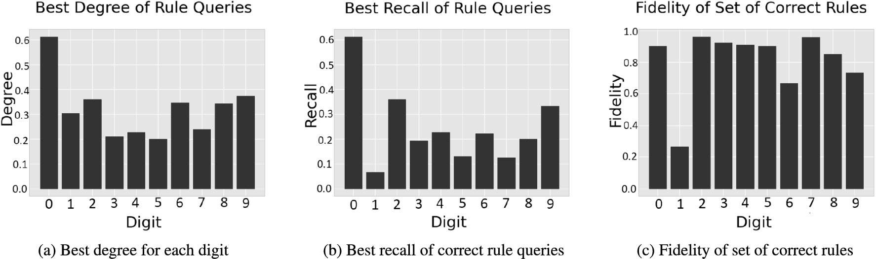
For all digits the algorithm produced at least one correct rule (precision = 1) and a rule with exceptions with recall = 1. The highest degree of rule queries for each digit are shown as a bar-plot in Fig. 12a. In general, the values of the metric seem low, with the exception of digit 0, which would indicate that the algorithms did not find a single rule which approximates the pos-set to a high degree. For some of the digits, including 0, the highest degree rule is also a correct rule. For closer inspection, we show the best degree rule query for digit 0 which is the highest, and for digit 5 which is the lowest.
Fig. 12.
Metrics of generated rule queries for MNIST.
The explanation rule for digit 0 involved six lines, as indicated by the conjuncts
Fig. 13.
Visualizations of best recall correct rules for digits.
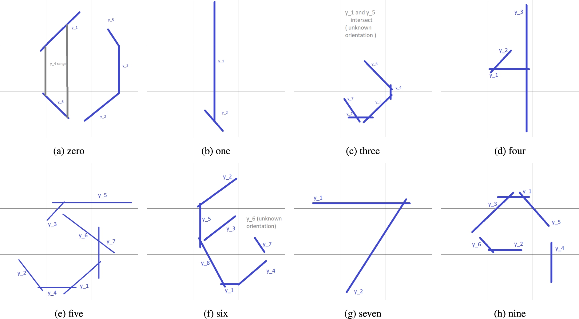
Fig. 14.
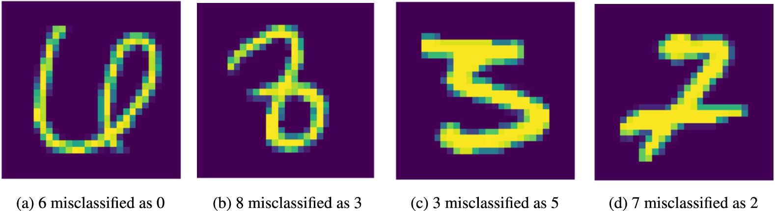
Misclassified digits that follow the best recall correct rules.
The highest degree explanation rule for digit 5, which was the lowest out of the best of all digits, again involved six lines indicated by the conjuncts
Regarding correct rules, the algorithm produced several for each digit. Since the sets of certain answers of correct rule queries are subsets of the pos-set of each class, we measured the per class fidelity of the disjunction of all correct rules, as if giving a user a rule-set, similarly to the Mushroom experiment (Section 5.1). In Fig. 12c we show as a bar-plot the fidelity for each class. With the exception of digit one, the pos-sets of all digits were sufficiently covered by the set of correct rules. The failure for digit 1 was expected, since the descriptions of the exemplars classified as 1 contain few lines (for example consisting of a single large line in the middle) which tend to be part of descriptions of other digits as well (all digits could be drawn in a way in which there is a single line in the middle). This is a drawback of the open world assumption of DLs since we cannot guarantee the non-existence of lines that are not provided in the descriptions. The open world assumption is still desirable since it allows for incomplete descriptions of exemplars. In cases such as the medical motivating example used throughout this paper, a missing finding such as “Dyspnoea” does not always imply that the patient does not suffer from dyspnoea. It could also be a symptom that has not been detected or has been overlooked.
The highest recall of a single correct rule for each digit is shown as a bar-plot in Fig. 12b. Since correct rules are easily translated into IF-THEN rules, we expected them to be more informative than the highest degree ones, which requires looking at the exceptions to gain a clearer understanding of the rule. We investigate closer by analyzing the best correct rule for each digit.
For digit 0, the best correct rule was the same as the highest degree rule presented previously. In Fig. 14a we provide an example of a six misclassified as a 0, which follows this correct rule. Comparing the misclassified 6 with the visualizations for rules of the digits 0 (Fig. 13a) and 6 (Fig. 13f) we can see that this 6 might have been misclassified as a 0 because the closed loop part of the digit reaches the top of the image. According to the correct rule for 0, an image that contains two vertical semicircles in the left and right sides of the image is classified as a 0, and because of this peculiarity in the drawing of the misclassified six, the image (Fig. 13a) obeys this rule.
The best correct rule for digit 1 had the lowest recall out of all correct rules for other digits, which means that it returned a small subset of the positives. Specifically, this rule returned only two of the 30 individuals classified as the digit 1. It was still usable as an explanation however, as it only involved two lines
For digit 2, the best correct rule query returned nine out of the 25 positives, three of which were missclassified by the classifier. This rule involved three lines, of which two had conjuncts indicating their location
To investigate closer, the next correct rule which we analyze is that of highest recall for digit 7. This query returned only three of the 24 images which were classified as sevens, and all three were correct predictions by the classifier. The rule involved two intersecting lines (
For digit 3, the best correct explanation rule returned five of the 26 individuals which were classified as 3, including one misclassified 8. This rule involved seven different lines, thus it was not expected to be understandable by a user at a glance. However, there was plentiful information for each line in the rule, which made it possible to visualize. Specifically, regarding the location of the lines, the rule query contained the conjuncts
For the digit 5, the best correct rule query returned four of the 31 positives for the class of which one is a misclassified 3. It is a very specific query involving seven lines, all of which are described regarding their orientation
For the digit 4, the best correct rule query returned five of the 22 positives all of which were correct predictions. The query involved three lines which were all well described regarding their orientation
For the digit 6, the best resulting correct rule involved the most variables (each representing a line) out of all correct rules. It returned four of the 18 positives for the class all of which were correct predictions. Of the eight lines described in the query, seven had information about their orientation
For digit 8, the best correct rule query returned four of the 20 positives, all of which are classified correctly. It involved seven lines, of which five were described with respect to their orientation
Finally, the best correct rule query for digit 9 returned five of the 15 positives, of which all were correct predictions by the classifier. It involved six lines which were all thoroughly described regarding their orientation
5.5.Discussion
The proposed approach performed similarly with the state-of-the-art on tabular data, was able to detect biases in the CLEVR-Hans case, detect flaws of the classifier in the Visual Genome case, and provided meaningful explanations even in the MNIST case. In this framework, the resulting explanations depend (almost exclusively) on the properties of the explanation dataset. In an ideal scenario, end-users trust the explanation dataset, the information it provides about the exemplars and the terminology it uses. It is like a quiz, or an exam, for the black-box, which is carefully curated by domain experts. This scenario was simulated in the CLEVR-Hans3 and Visual Genome use-cases in which the set of rules produced by the proposed algorithms clearly showed in which cases the black-box classifies items in specific classes, highlighting potential biases acquired during training. The framework is also useful when the explanation dataset is created automatically by leveraging traditional feature extraction, as is shown in the MNIST use-case. In this case, we found the resulting queries to be less understandable than before, which stems mainly from the vocabulary used, since sets of intersecting lines are not easily understandable unless they are visualized. They are also subjectively less trustworthy, since there are usually flaws with most automatic information extraction procedures. However, since sets of correct rules sufficiently covered the sets of individuals, and rules with exceptions achieved decent performance regarding precision, recall and degree, if an end-user invested time and effort to analyze the resulting rules, they could get a more clear picture about what the black-box is doing.
We also found interesting the comparison of correct rules with those with exceptions. Correct rules are, in general, more specific than others, as they always have a subset of the pos-set as certain answers. This means that, even though they might be more informative, they tend to involve more conjuncts than rules with exceptions, which in extreme cases could impact understandability. On the other hand, rules with exceptions can be more general, with fewer conjuncts, which could positively impact understandability. Although, utilizing these rules should involve examining the actual exceptions, which could be a lot of work for an end-user, we believe that these exceptions themselves can be very useful in order to detect biases and investigate the behaviour of the model on outliers. In order to eliminate the complexity involved in the investigation of these exceptions, in the future we plan to further study the area and propose a systematic way of exploiting them. These conclusions were apparent in the explanations generated for the class 3 of CLEVR-Hans3 (Table 6), where the best correct rule was very specific, involved five objects and had a relatively low recall (0.42), while the best rule with exceptions was exactly the ground truth class description and had very high precision (0.99). So in this case a user would probably gain more information about the classifier if they examined the rule with exceptions along with the few false positives, instead of examining the best correct rule, or a set of correct rules.
Another observation we made, is the fact that some conjuncts were more understandable than others when they were part of explanation rules. For instance in MNIST, knowing a line’s location and orientation was imperative for understanding the rule via visualization, while conjuncts involving line intersections and sizes seemed not that important, regardless of metrics. This is something which could be leveraged either in explanation dataset construction (for example domain experts weigh concepts and roles depending on their importance for understandability), or in algorithm design (for example a user could provide as input concepts and roles which they want to appear in explanation rules). We are considering these ideas as a main direction for future work which involves developing strategies for choosing which rules are best to show to a user.
Finally, in the first experiment (Section 5.1), it is shown that KGrules-H can be used to generate explanations in terms of feature data similarly to other rule-based methods, even if it is not the intended use-case. An interesting comparison for a user study would be between different vocabularies (for example using the features vs using external knowledge). We note here that the proposed approach can always be applied on categorical feature data, since their transformation to an explanation dataset is straight-forward. This would not be the case if we also had numerical continuous features, in which case we would either require more expressive knowledge to represent these features, or that the continuous features be discretized. Another result which motivates us to explore different knowledge expressivities in the future, was the failure of the algorithms to produce a good (w.r.t. the metrics) explanation for the digit 1 in the MNIST experiment (Section 5.4). Specifically, it was difficult to find a query which only returns images of this digit, since a typical description of a “1” is general and tends to always partially describe other digits. This is something which could be mitigated if we allowed for negation in the generated rules, and this is the second direction which we plan to explore in the future.
6.Conclusions and future work
In this work we have further developed a framework for rule-based post hoc explanations of black-box classifiers. The explanations are expressed as Horn rules which use terms from a given vocabulary, instead of the classifier’s features. This allows for intuitive explanations even when the feature space of the classifier is too complex to be used within understandable rules (pixels, audio signals etc). The rules are also accompanied by theoretical guarantees regarding their correctness for explaining the classifier, given what we call an explanation dataset. The idea of the explanation dataset is at the core of our framework, as it is the probe we use to observe the black-box, by feeding it exemplar data and finding rules which explain its output. The explanation dataset also contains the knowledge from which the semantics of the rules are derived. The problem of finding such rules given an explanation dataset was approached as a search problem in the space of semantic queries, by starting with the most specific queries describing positively classified exemplars, and then progressively merging them using heuristic criteria. The queries are then approximately condensed, converted to rules and are shown to the end-user.
There are multiple directions towards which we plan to extend the framework in the future. First of all, we are currently investigating different strategies for choosing which explanation rules are best to show to a user such that they are both informative and understandable. To do this, we also plan to extend our evaluation framework for real world applications to include user studies. Specifically, we are focusing on decision critical domains in which explainability is crucial, such as the medical domain, and in collaboration with domain experts, we are developing explanation datasets, in addition to a crowd-sourced explanation evaluation platform. There are many interesting research questions which we are exploring in this context, such as what constitutes a good explanation dataset, what is a good explanation, and how can we build the trust required for opaque AI to be utilized in such applications.
Another direction which we are currently exploring involves further investigation of our framework in order to fully exploit its capabilities. In particular, the existence of exceptions might have a large impact on both understandability of the produced explanations, and their ability to approximate the behavior of the black-box model.
We believe that the systematic study of exceptions could provide useful information to the end-user regarding biases and outliers, and could drive the way towards incorporating local explanations to our framework. Stemming from this, we want to extend the framework, both in theory and in practice, to incorporate different types of explanations. This includes local explanations which explain individual predictions of the black-box, and counterfactual or contrastive explanations which highlight how a specific input should be modified in order for the prediction of the classifier to change. This extension is being researched with the end-user in mind, and we are exploring the merits of providing a blend of explanations (global, local, counterfactual) to an end-user.
A fourth and final direction to be explored involves extending the expressivity of explanation rules, in addition to that of the underlying knowledge. Specifically, the algorithms developed in this work require that if the knowledge has a non-empty TBox, it has to be eliminated via materialization before running the algorithms. Thus, we are exploring ideas for algorithms which generate explanation rules in the case where the underlying knowledge is represented with DL dialects in which the TBox cannot be eliminated, such as DL_Lite. Finally, regarding the expressivity of explanation rules, we plan to extend the framework to allow for disjunction, which is a straight-forward extension, and for negation, which is much harder to incorporate in the framework while maintaining the theoretical guarantees, which we believe are crucial for building trust with end-users.
Notes
1 All code and data are available at https://github.com/ails-lab/kgrules-h.
7 PyTorch model: http://places2.csail.mit.edu/models_places365/resnet50_places365.pth.tar.
References
[1] | Q. Ai, V. Azizi, X. Chen and Y. Zhang, Learning heterogeneous knowledge base embeddings for explainable recommendation, Algorithms 11: (9) ((2018) ), 137. doi:10.3390/a11090137. |
[2] | M. Alirezaie, M. Längkvist, M. Sioutis and A. Loutfi, A symbolic approach for explaining errors in image classification tasks, 2018, https://www.diva-portal.org/smash/record.jsf?pid=diva2%3A1233674&dswid=-9184. |
[3] | M. Arenas, G.I. Diaz and E.V. Kostylev, Reverse engineering SPARQL queries, in: Proceedings of the 25th International Conference on World Wide Web, J. Bourdeau, J. Hendler, R. Nkambou, I. Horrocks and B.Y. Zhao, eds, WWW’16, International World Wide Web Conferences Steering Committee, Republic and Canton of Geneva, CHE, (2016) , pp. 239–249. doi:10.1145/2872427.2882989. |
[4] | A.B. Arrieta, N.D. Rodríguez, J.D. Ser, A. Bennetot, S. Tabik, A. Barbado, S. García, S. Gil-Lopez, D. Molina, R. Benjamins, R. Chatila and F. Herrera, Explainable artificial intelligence (XAI): Concepts, taxonomies, opportunities and challenges toward responsible AI, Information Fusion 58: ((2020) ), 82–115, https://www.sciencedirect.com/science/article/pii/S1566253519308103. doi:10.1016/j.inffus.2019.12.012. |
[5] | F. Baader, D. Calvanese, D.L. McGuinness, D. Nardi and P.F. Patel-Schneider (eds), The Description Logic Handbook: Theory, Implementation, and Applications, Cambridge University Press, Cambridge, United Kingdom, (2003) . doi:10.1017/CBO9780511711787. |
[6] | F. Baader, B. Sertkaya and A. Turhan, Computing the least common subsumer w.r.t. a background terminology, Journal of Applied Logic 5: (3) ((2007) ), 392–420. doi:10.1016/j.jal.2006.03.002. |
[7] | P. Barceló and M. Romero, The complexity of reverse engineering problems for conjunctive queries, in: 20th International Conference on Database Theory (ICDT 2017), Vol. 68, (2017) , 7:1–7:17, ISBN 978-3-95977-024-8. doi:10.4230/LIPIcs.ICDT.2017.7. http://drops.dagstuhl.de/opus/volltexte/2017/7052. |
[8] | S.H. Bokhari, On the mapping problem, IEEE Transactions on Computers C-30: (3) ((1981) ), 207–214. doi:10.1109/TC.1981.1675756. |
[9] | A. Bonifati, R. Ciucanu and S. Staworko, Learning join queries from user examples, ACM Transactions on Database Systems 40: (4) ((2016) ). doi:10.1145/2818637. |
[10] | D. Calvanese, G.D. Giacomo, D. Lembo, M. Lenzerini and R. Rosati, Tractable reasoning and efficient query answering in description logics: The DL-lite family, Journal of Automated Reasoning 39: (3) ((2007) ), 385–429. doi:10.1007/s10817-007-9078-x. |
[11] | A. Chortaras, M. Giazitzoglou and G. Stamou, Inside the query space of DL knowledge bases, in: Proceedings of the 32nd International Workshop on Description Logics, M. Šimkus and G. Weddell, eds, International Workshop on Description Logics, Vol. 2373: , CEUR-WS.org, Aachen, Germany, (2019) , https://ceur-ws.org/Vol-2373/paper-11.pdf. |
[12] | G. Cima, F. Croce and M. Lenzerini, Query definability and its approximations in ontology-based data management, in: CIKM’21, Association for Computing Machinery, New York, NY, USA, (2021) , pp. 271–280. ISBN 9781450384469. doi:10.1145/3459637.3482466. |
[13] | G. Ciravegna, F. Giannini, M. Gori, M. Maggini and S. Melacci, Human-driven FOL explanations of deep learning, in: Proceedings of the Twenty-Ninth International Joint Conference on Artificial Intelligence, IJCAI-20, C. Bessiere, ed., International Joint Conferences on Artificial Intelligence Organization, (2020) , pp. 2234–2240, Main track. doi:10.24963/ijcai.2020/309. |
[14] | W.W. Cohen, A. Borgida and H. Hirsh, Computing least common subsumers in description logics, in: Proceedings of the 10th National Conference on Artificial Intelligence, AAAI Press, Palo Alto, California, USA, (1992) , pp. 754–760, https://aaai.org/papers/00754-computing-least-common-subsumers-in-description-logics/. |
[15] | R. Confalonieri, T. Weyde, T.R. Besold and F. Moscoso del Prado Martín, Using ontologies to enhance human understandability of global post-hoc explanations of black-box models, Artificial Intelligence 296: ((2021) ), 103471, https://www.sciencedirect.com/science/article/pii/S0004370221000229. doi:10.1016/j.artint.2021.103471. |
[16] | M.W. Craven and J.W. Shavlik, Extracting tree-structured representations of trained networks, in: Advances in Neural Information Processing Systems, D. Touretzky, M.C. Mozer and M. Hasselmo, eds, Vol. 8: , MIT Press, (1995) , pp. 24–30, http://papers.nips.cc/paper/1152-extracting-tree-structured-representations-of-trained-networks. |
[17] | F. Croce, G. Cima, M. Lenzerini and T. Catarci, Ontology-based explanation of classifiers, in: CEUR Workshop Proceedings, Vol. 2578: , CEUR-WS.org, (2020) , https://ceur-ws.org/Vol-2578/PIE3.pdf. |
[18] | Z.A. Daniels, L.D. Frank, C.J. Menart, M. Raymer and P. Hitzler, A framework for explainable deep neural models using external knowledge graphs, in: Artificial Intelligence and Machine Learning for Multi-Domain Operations Applications II, International Society for Optics and Photonics, Vol. 11413: , SPIE, (2020) , p. 114131C. doi:10.1117/12.2558083. |
[19] | E. Dervakos, O. Menis-Mastromichalakis, A. Chortaras and G. Stamou, Computing rule-based explanations of machine learning classifiers using knowledge graphs, 2022. doi:10.48550/arXiv.2202.03971. |
[20] | G. Diaz, M. Arenas and M. Benedikt, SPARQLByE: Querying RDF data by example, 9: (13) ((2016) ), 1533–1536. doi:10.14778/3007263.3007302. |
[21] | F.M. Donini, S. Colucci, T.D. Noia and E.D. Sciascio, A tableaux-based method for computing least common subsumers for expressive description logics, in: Proceedings of the 22nd International Workshop on Description Logics (DL 2009), B.C. Grau, I. Horrocks, B. Motik and U. Sattler, eds, CEUR-WS.org, (2009) , http://ceur-ws.org/Vol-477/paper_22.pdf. |
[22] | A. Egozi, Y. Keller and H. Guterman, A probabilistic approach to spectral graph matching, IEEE Transactions on Pattern Analysis and Machine Intelligence 35: (01) ((2013) ), 18–27. doi:10.1109/TPAMI.2012.51. |
[23] | G. Filandrianos, K. Thomas, E. Dervakos and G. Stamou, Conceptual edits as counterfactual explanations, in: Proceedings of the AAAI 2022 Spring Symposium on Machine Learning and Knowledge Engineering for Hybrid Intelligence (AAAI-MAKE 2022), A. Martin, K. Hinkelmann, H.-G. Fill, A. Gerber, D. Lenat, R. Stolle and F. van Harmelen, eds, CEUR Workshop Proceedings, CEUR-WS.org, Palo Alto, California, USA, (2022) , https://ceur-ws.org/Vol-3121/paper6.pdf. |
[24] | G. Futia and A. Vetrò, On the integration of knowledge graphs into deep learning models for a more comprehensible AI – three challenges for future research, Information 11: (2) ((2020) ), 122. doi:10.3390/info11020122. |
[25] | B. Glimm, Y. Kazakov and T. Tran, Ontology Materialization by Abstraction Refinement in Horn SHOIF, AAAI Press, Palo Alto, California, USA, (2017) , pp. 1114–1120. doi:10.1609/aaai.v31i1.10691. |
[26] | B. Goodman and S.R. Flaxman, European Union regulations on algorithmic decision-making and a “right to explanation”, AI Magazine 38: (3) ((2017) ), 50–57. doi:10.1609/aimag.v38i3.2741. |
[27] | G. Gottlob and C.G. Fermüller, Removing redundancy from a clause, Artificial Intelligence 61: (2) ((1993) ), 263–289. doi:10.1016/0004-3702(93)90069-N. |
[28] | B.C. Grau, B. Motik, G. Stoilos and I. Horrocks, Computing datalog rewritings beyond Horn ontologies, in: IJCAI, Menlo Park, California, USA, F. Rossi, ed., AAAI Press / International Joint Conferences on Artificial Intelligence (2013) , pp. 832–838, https://www.ijcai.org/Proceedings/13/Papers/129.pdf. |
[29] | H.M. Grindley, P.J. Artymiuk, D.W. Rice and P. Willett, Identification of tertiary structure resemblance in proteins using a maximal common subgraph isomorphism algorithm, Journal of Molecular Biology 229: (3) ((1993) ), 707–721, https://www.sciencedirect.com/science/article/pii/S0022283683710740. doi:10.1006/jmbi.1993.1074. |
[30] | R. Guidotti, A. Monreale, S. Ruggieri, D. Pedreschi, F. Turini and F. Giannotti, Local rule-based explanations of black box decision systems, arXiv preprint arXiv:1805.10820, 2018. doi:10.48550/arXiv.1805.10820. |
[31] | R. Guidotti, A. Monreale, S. Ruggieri, F. Turini, F. Giannotti and D. Pedreschi, A survey of methods for explaining black box models, ACM Computing Surveys 51: (5) ((2019) ), 93:1–93:42. doi:10.1145/3236009. |
[32] | V. Gutiérrez-Basulto, J.C. Jung and L. Sabellek, Reverse engineering queries in ontology-enriched systems: The case of expressive Horn description logic ontologies, in: Proceedings of the Twenty-Seventh International Joint Conference on Artificial Intelligence, IJCAI-18, International Joint Conferences on Artificial Intelligence Organization, (2018) , pp. 1847–1853. doi:10.24963/ijcai.2018/255. |
[33] | K. He, X. Zhang, S. Ren and J. Sun, Deep Residual Learning for Image Recognition ((2015) ). doi:10.48550/arXiv.1512.03385. |
[34] | A. Hogan, E. Blomqvist, M. Cochez, C. d’Amato, G. de Melo, C. Gutiérrez, J.E.L. Gayo, S. Kirrane, S. Neumaier, A. Polleres, R. Navigli, A.N. Ngomo, S.M. Rashid, A. Rula, L. Schmelzeisen, J.F. Sequeda, S. Staab and A. Zimmermann, Knowledge graphs, ACM Computing Surveys 54: ((2020) ). doi:10.1145/3447772. |
[35] | J. Johnson, B. Hariharan, L. van der Maaten, L. Fei-Fei, C.L. Zitnick and R.B. Girshick, CLEVR: A Diagnostic Dataset for Compositional Language and Elementary Visual Reasoning, (2016) . doi:10.48550/arXiv.1612.06890. |
[36] | J. Jung, C. Lutz, H. Pulcini and F. Wolter, Logical separability of incomplete data under ontologies, in: Proceedings of the 17th International Conference on Principles of Knowledge Representation and Reasoning, D. Calvanese, E. Erdem and M. Thielscher, eds, IJCAI Organization, (2020) , pp. 517–528. doi:10.24963/kr.2020/52. |
[37] | R. Kontchakov, C. Lutz, D. Toman, F. Wolter and M. Zakharyaschev, The combined approach to ontology-based data access, in: AAAI Press/International Joint Conferences on Artificial Intelligence, T. Walsh, ed., Menlo Park, California, USA, (2011) , pp. 2656–2661. doi:10.5591/978-1-57735-516-8/IJCAI11-442. |
[38] | R. Kontchakov and M. Zakharyaschev, An introduction to description logics and query rewriting, in: Reasoning Web. Reasoning on the Web in the Big Data Era: 10th International Summer School 2014, Proceedings, M. Koubarakis, G. Stamou, G. Stoilos, I. Horrocks, P. Kolaitis, G. Lausen and G. Weikum, eds, Lecture Notes in Computer Science, Vol. 8714: , Springer International Publishing, Cham, (2014) , pp. 195–244. ISBN 978-3-319-10587-1. doi:10.1007/978-3-319-10587-1_5. |
[39] | R. Krishna, Y. Zhu, O. Groth, J. Johnson, K. Hata, J. Kravitz, S. Chen, Y. Kalantidis, L.-J. Li, D.A. Shamma et al., Visual genome: Connecting language and vision using crowdsourced dense image annotations, International journal of computer vision 123: (1) ((2017) ), 32–73. doi:10.1007/s11263-016-0981-7. |
[40] | R. Küsters and R. Molitor, Structural subsumption and least common subsumers in a description logic with existential and number restrictions, Studia Logica 81: (2) ((2005) ), 227–259. doi:10.1007/s11225-005-3705-5. |
[41] | J. Laguarta, F. Hueto and B. Subirana, COVID-19 artificial intelligence diagnosis using only cough recordings, IEEE Open Journal of Engineering in Medicine and Biology 1: ((2020) ), 275–281. doi:10.1109/OJEMB.2020.3026928. |
[42] | F. Lecue, On the role of knowledge graphs in explainable AI, Semantic Web 11: ((2020) ), 41–51. doi:10.3233/SW-190374. |
[43] | Y. LeCun, L. Bottou, Y. Bengio and P. Haffner, Gradient-based learning applied to document recognition, in: Proceedings of the IEEE, G. Setti, ed., Vol. 86: , IEEE, (1998) , pp. 2278–2324. doi:10.1109/5.726791. |
[44] | J. Lehmann, S. Bader and P. Hitzler, Extracting reduced logic programs from artificial neural networks, Applied Intelligence 32: (3) ((2010) ), 249–266. doi:10.1007/s10489-008-0142-y. |
[45] | J. Lehmann, R. Isele, M. Jakob, A. Jentzsch, D. Kontokostas, P.N. Mendes, S. Hellmann, M. Morsey, P. Van Kleef, S. Auer et al., Dbpedia – a large-scale, multilingual knowledge base extracted from Wikipedia, Semantic web 6: (2) ((2015) ), 167–195. doi:10.3233/SW-140134. |
[46] | M. Leordeanu and M. Hebert, A spectral technique for correspondence problems using pairwise constraints, in: Tenth IEEE International Conference on Computer Vision (ICCV’05), Vol. 1, Vol. 2, IEEE, (2005) , pp. 1482–1489. doi:10.1109/ICCV.2005.20. |
[47] | H. Li, C.-Y. Chan and D. Maier, Query from examples: An iterative, data-driven approach to query construction, Proceedings of the VLDB Endowment 8: (13) ((2015) ), 2158–2169. doi:10.14778/2831360.2831369. |
[48] | J. Liartis, E. Dervakos, O. Menis-Mastromichalakis, A. Chortaras and G. Stamou, Semantic queries explaining opaque machine learning classifiers, in: Proceedings of the Workshop on Data Meets Applied Ontologies in Explainable AI (DAO-XAI 2021), R. Confalonieri, O. Kutz and D. Calvanese, eds, CEUR Workshop Proceedings, Vol. 2998: , CEUR-WS.org, (2021) , http://ceur-ws.org/Vol-2998/paper2.pdf. |
[49] | T.-Y. Lin, M. Maire, S. Belongie, J. Hays, P. Perona, D. Ramanan, P. Dollár and C.L. Zitnick, Microsoft coco: Common Objects in Context, in: Lecture Notes in Computer Science, Vol. 8693: , Springer, (2014) , pp. 740–755. doi:10.1007/978-3-319-10602-1_48. |
[50] | T. Lindeberg, Scale–space, in: Wiley Encyclopedia of Computer Science and Engineering, B.W. Wah, ed., John Wiley & Sons, Ltd, (2008) , pp. 2495–2504. ISBN 9780470050118. doi:10.1002/9780470050118.ecse609. |
[51] | D.M.L. Martins, Reverse engineering database queries from examples: State-of-the-art, challenges, and research opportunities, Information Systems 83: ((2019) ), 89–100, https://www.sciencedirect.com/science/article/pii/S0306437918300978. doi:10.1016/j.is.2019.03.002. |
[52] | G.A. Miller, WordNet: A lexical database for English, Communications of the ACM 38: (11) ((1995) ), 39–41. doi:10.1145/219717.219748. |
[53] | Y. Ming, H. Qu and E. Bertini, RuleMatrix: Visualizing and understanding classifiers with rules, IEEE Transactions on Visualization and Computer Graphics 25: (1) ((2019) ), 342–352. doi:10.1109/TVCG.2018.2864812. |
[54] | B. Mittelstadt, C. Russell and S. Wachter, Explaining explanations in AI, in: Proceedings of the Conference on Fairness, Accountability, and Transparency, Association for Computing Machinery, New York, NY, USA, (2019) , pp. 279–288. doi:10.1145/3287560.3287574. |
[55] | W.J. Murdoch, C. Singh, K. Kumbier, R. Abbasi-Asl and B. Yu, Definitions, methods, and applications in interpretable machine learning, Proceedings of the National Academy of Sciences 116: (44) ((2019) ), 22071–22080. doi:10.1073/pnas.1900654116. |
[56] | M. Ortiz, Ontology-mediated queries from examples: A glimpse at the DL-lite case, in: GCAI 2019. Proceedings of the 5th Global Conference on Artificial Intelligence, D. Calvanese and L. Iocchi, eds, EPiC Series in Computing, Vol. 65: , EasyChair, (2019) , pp. 1–14, ISSN 2398-7340, https://easychair.org/publications/paper/c3CT. doi:10.29007/jhtz. |
[57] | C. Panigutti, A. Perotti and D. Pedreschi, Doctor XAI: An ontology-based approach to black-box sequential data classification explanations, in: Proceedings of the 2020 Conference on Fairness, Accountability, and Transparency, Association for Computing Machinery, New York, NY, USA, (2020) , pp. 629–639. doi:10.1145/3351095.3372855. |
[58] | D. Pedreschi, F. Giannotti, R. Guidotti, A. Monreale, S. Ruggieri and F. Turini, Meaningful Explanations of Black Box AI Decision Systems, AAAI Press, Palo Alto, California USA, (2019) , pp. 9780–9784. doi:10.1609/aaai.v33i01.33019780. |
[59] | A. Petrova, E.V. Kostylev, B.C. Grau and I. Horrocks, Query-based entity comparison in knowledge graphs revisited, in: The Semantic Web – ISWC 2019 – 18th International Semantic Web Conference, Auckland, New Zealand, October 26–30, 2019, Proceedings, Part I, C. Ghidini, O. Hartig, M. Maleshkova, V. Svátek, I.F. Cruz, A. Hogan, J. Song, M. Lefrançois and F. Gandon, eds, Lecture Notes in Computer Science, Vol. 11778: , Springer, (2019) , pp. 558–575. doi:10.1007/978-3-030-30793-6_32. |
[60] | R. Poyiadzi, K. Sokol, R. Santos-Rodríguez, T.D. Bie and P.A. Flach, FACE: Feasible and Actionable Counterfactual Explanations, in AIES’20, Association for Computing Machinery, New York, NY, USA, (2020) , pp. 344–350. doi:10.1145/3375627.3375850. |
[61] | V. Praher, K. Prinz, A. Flexer and G. Widmer, On the veracity of local, model-agnostic explanations in audio classification: Targeted investigations with adversarial examples, arXiv preprint, 2021. doi:10.48550/arXiv.2107.09045. |
[62] | M.T. Ribeiro, S. Singh and C. Guestrin, Anchors: High-precision model-agnostic explanations, in: Proceedings of the AAAI Conference on Artificial Intelligence, Vol. 32: , Public Knowledge Project, (2018) . doi:10.1609/aaai.v32i1.11491. |
[63] | C. Rudin, Stop explaining black box machine learning models for high stakes decisions and use interpretable models instead, Nature Machine Intelligence 1: (5) ((2019) ), 206–215. doi:10.1038/s42256-019-0048-x. |
[64] | M.K. Sarker, N. Xie, D. Doran, M. Raymer and P. Hitzler, Explaining trained neural networks with semantic web technologies: First steps, in: Neural-Symbolic Learning and Reasoning 2017, T.R. Besold, A.d. Garcez and I. Noble, eds, CEUR Workshop Proceedings, Vol. 2003: , CEUR-WS.org, Aachen, Germany, (2017) , https://ceur-ws.org/Vol-2003/NeSy17_paper4.pdf. |
[65] | V.S. Silva, A. Freitas and S. Handschuh, Exploring Knowledge Graphs in an Interpretable Composite Approach for Text Entailment, AAAI Press, Palo Alto, California, USA, (2019) , pp. 7023–7030. doi:10.1609/aaai.v33i01.33017023. |
[66] | R. Speer, J. Chin and C. Havasi, ConceptNet 5.5: An Open Multilingual Graph of General Knowledge, (2016) . doi:10.48550/arXiv.1612.03975. |
[67] | R. Speer, J. Chin and C. Havasi, ConceptNet 5.5: An Open Multilingual Graph of General Knowledge, Association for the Advancement of Artificial Intelligence, Washington, DC, USA, (2017) , pp. 4444–4451, https://dl.acm.org/doi/10.5555/3298023.3298212. |
[68] | W. Stammer, P. Schramowski and K. Kersting, Right for the right concept: Revising neuro-symbolic concepts by interacting with their explanations, arXiv preprint, 2020. doi:10.48550/arXiv.2011.12854. |
[69] | M.Q. Stearns, C. Price, K.A. Spackman and A.Y. Wang, SNOMED Clinical Terms: Overview of the Development Process and Project Status, S. Bakken, ed., Hanley & Belfus Inc., Northfield, IL, USA, (2001) , pp. 662–666, https://www.ncbi.nlm.nih.gov/pmc/articles/PMC2243297/. |
[70] | B. ten Cate and V. Dalmau, The product homomorphism problem and applications, in: 18th International Conference on Database Theory (ICDT 2015), M. Arenas and M. Ugarte, eds, Leibniz International Proceedings in Informatics (LIPIcs), Vol. 31: , Schloss Dagstuhl–Leibniz-Zentrum fuer Informatik, Dagstuhl, Germany, (2015) , pp. 161–176. ISSN 1868-8969. http://drops.dagstuhl.de/opus/volltexte/2015/4983. ISBN 978-3-939897-79-8. doi:10.4230/LIPIcs.ICDT.2015.161. |
[71] | I. Tiddi and S. Schlobach, Knowledge graphs as tools for explainable machine learning: A survey, Artificial Intelligence 302: ((2022) ), 103627. doi:10.1016/j.artint.2021.103627. |
[72] | Q.T. Tran, C.Y. Chan and S. Parthasarathy, Query reverse engineering, The VLDB Journal 23: (5) ((2014) ), 721–746. doi:10.1007/s00778-013-0349-3. |
[73] | D. Trivela, G. Stoilos, A. Chortaras and G. Stamou, Resolution-based rewriting for Horn-SHIQ ontologies, Knowledge and Information Systems 62: (1) ((2020) ), 107–143. doi:10.1007/s10115-019-01345-2. |
[74] | M. Turek, Explainable artificial intelligence (XAI), Defense Advanced Research Projects Agency, (2018) , https://www.darpa.mil/program/explainable-artificial-intelligence. |
[75] | J. van der Waa, E. Nieuwburg, A. Cremers and M. Neerincx, Evaluating XAI: A comparison of rule-based and example-based explanations, Artificial Intelligence 291: ((2021) ), 103404. doi:10.1016/j.artint.2020.103404. |
[76] | C. Wang, A. Cheung and R. Bodik, Synthesizing highly expressive SQL queries from input-output examples, SIGPLAN Not. 52: (6) ((2017) ), 452–466. doi:10.1145/3140587.3062365. |
[77] | H. Wang, Z. Wang, M. Du, F. Yang, Z. Zhang, S. Ding, P. Mardziel and X. Hu, Score-CAM: Score-weighted visual explanations for convolutional neural networks, arXiv, 2019, https://arxiv.org/abs/1910.01279. doi:10.48550/ARXIV.1910.01279. |
[78] | H. Wang, F. Zhang, X. Xie and M. Guo, DKN: Deep knowledge-aware network for news recommendation, in: Proceedings of the 2018 World Wide Web Conference on World Wide Web, International World Wide Web Conferences Steering Committee, Republic and Canton of Geneva, CHE, (2018) , pp. 1835–1844. doi:10.1145/3178876.3186175. |
[79] | J. Xu, GMA: A generic match algorithm for structural homomorphism, isomorphism, and maximal common substructure match and its applications, Journal of Chemical Information and Computer Sciences 36: (1) ((1996) ), 25–34. doi:10.1021/ci950061u. |
[80] | H. Yang, C. Rudin and M. Seltzer, Scalable Bayesian rule lists, in: Proceedings of the 34th International Conference on Machine Learning, D. Precup and Y.W. Teh, eds, Proceedings of Machine Learning Research, Vol. 70: , PMLR, (2017) , pp. 3921–3930, https://proceedings.mlr.press/v70/yang17h.html. |
[81] | M. Zhang, H. Elmeleegy, C.M. Procopiuc and D. Srivastava, Reverse engineering complex join queries, in: Proceedings of the 2013 ACM SIGMOD International Conference on Management of Data, SIGMOD’13, Association for Computing Machinery, New York, NY, USA, (2013) , pp. 809–820. ISBN 9781450320375. doi:10.1145/2463676.2465320. |
[82] | Y. Zhang, P. Tiño, A. Leonardis and K. Tang, A survey on neural network interpretability, IEEE Transactions on Emerging Topics in Computational Intelligence 5: (5) ((2021) ), 726–742. doi:10.1109/TETCI.2021.3100641. |
[83] | B. Zhou, A. Lapedriza, A. Khosla, A. Oliva and A. Torralba, Places: A 10 million image database for scene recognition, IEEE transactions on pattern analysis and machine intelligence 40: (6) ((2017) ), 1452–1464. doi:10.1109/TPAMI.2017.2723009. |
[84] | Y. Zhou and G. Hooker, Interpreting models via single tree approximation, arXiv preprint arXiv:1610.09036, 2016. doi:10.48550/arXiv.1610.09036. |
[85] | M.M. Zloof, Query-by-example: The invocation and definition of tables and forms, in: VLDB’75, Association for Computing Machinery, New York, NY, USA, (1975) . doi:10.1145/1282480.1282482. |

