


INTRODUCTION
Radiocarbon dating of marine shells from the coastline of New Zealand has been a vital chronological component of archaeological (Higham and Hogg Reference Higham and Hogg1995; Petchey and Schmid Reference Petchey and Schmid2020), coastal geomorphology (Woodroffe et al. Reference Woodroffe, Curtis and McLean1983; Shulmeister and Kirk Reference Shulmeister and Kirk1993), sea level (Gibb Reference Gibb1986; Clement et al. Reference Clement, Whitehouse and Sloss2016), and coastal hazards research (Berryman Reference Berryman1993; Hayward et al. Reference Hayward, Grenfell, Sabaa, Cochran, Clark, Wallace and Palmer2016; Dowling et al. Reference Dowling, Clark, Howarth, Litchfield and Cochran2018; Clark et al. Reference Clark, Howarth, Litchfield, Cochran, Turnbull, Dowling, Howell, Berryman and Wolfe2019; Litchfield et al. Reference Litchfield, Clark, Cochran, Palmer, Mountjoy, Mueller, Morgenstern, Berryman, McFadgen and Steele2020) for many decades. A common approach to calibrating marine radiocarbon samples from the New Zealand mainland coastline (excluding Chatham Islands, Figure 1A) has been to apply a New Zealand-wide average for the local radiocarbon (14C) marine reservoir correction (ΔR) (McFadgen and Manning Reference McFadgen and Manning1990; Petchey et al. Reference Petchey, Anderson, Hogg and Zondervan2008a), but prior to 2019, this average was derived from only 27 samples that were mostly clustered in four locations (Figure 1B). With a coastline spanning 15° latitude and complex oceanographic currents and fronts, it might seem unlikely there is homogeneity in the local marine reservoir correction of New Zealand mainland coastal waters (Figure 1A). However, the small sample size and lack of geographic coverage meant the suitability of a nation-wide average ΔR was hard to evaluate as regional variations could not be interrogated. Potential variations are important for research such as coastal paleoseismology, in which past coastal earthquakes and tsunamis are dated using marine samples and temporal correlations between sites constrain the size and impact of these past events (e.g., Berryman et al. Reference Berryman, Ota, Miyauchi, Hull, Clark, Ishibashi, Iso and Litchfield2011; Clark et al. Reference Clark, Howarth, Litchfield, Cochran, Turnbull, Dowling, Howell, Berryman and Wolfe2019; Howell and Clark Reference Howell and Clark2022). In recent years, uncertainty about the ΔR has hampered the precision with which past coastal earthquakes and tsunamis can be dated and correlated. Prior to 2019, there were no ΔR values along the entire eastern coastline of the North Island that lies adjacent to New Zealand’s largest seismic and tsunami source, the Hikurangi Subduction Zone.

Figure 1 (A) Map of New Zealand showing the coverage and ΔR values in the Marine Reservoir Correction Database prior to 2019 (Reimer and Reimer Reference Reimer and Reimer2001). Also shown are the major coastal currents and oceanographic fronts around the New Zealand shelf (Chiswell et al. Reference Chiswell, Bostock, Sutton and Williams2015; Stevens et al. Reference Stevens, O’Callaghan, Chiswell and Hadfield2021). EAUC: East Auckland Current, WE: Wairarapa Eddy, WCC: Wairarapa Coastal Current, HE: Hikurangi Eddy, dUC: d’Urville Current, WC: Westland Current, SC: Southland Current, TF: Tasman Front, STF: Subtropical Front, SAF: Subantarctic Front. (B) Location and sequential additions to the Marine Reservoir Correction Database from 1990–2008. Details on the number of samples and average ΔR are shown in Table 1. Black line indicates the range of locations that the fish otolith samples may have been taken from (see text for details). (C) Location of new ΔR values for New Zealand in this study.
A far better understanding of an appropriate ΔR for mainland coastal waters, tailored to the type of marine shell dated and locations of particular interest, is needed for the advancement of coastal hazard research in New Zealand. Although also beneficial in other disciplines (e.g., archaeology and sea level studies), here we focus on the needs of the coastal hazard research community. Coastal tectonic hazard research in New Zealand predominantly focuses on earthquakes that have uplifted or subsided the coastline, and palaeotsunamis that have inundated the land (e.g., Berryman et al. Reference Berryman, Ota, Miyauchi, Hull, Clark, Ishibashi, Iso and Litchfield2011, Reference Berryman, Clark, Cochran, Beu and Irwin2018; Litchfield et al. Reference Litchfield, Clark, Cochran, Palmer, Mountjoy, Mueller, Morgenstern, Berryman, McFadgen and Steele2020, Reference Litchfield, Morgenstern, Clark, Howell, Grant and Turnbull2023; Pizer et al. Reference Pizer, Clark, Howarth, Garrett, Wang, Rhoades and Woodroffe2021). Almost all of this research is focused on the mid to late Holocene (<∼7500 yr BP) from when post-glacial sea level rise stabilized to within ± 2 m of its current elevation (Clement et al. Reference Clement, Whitehouse and Sloss2016). In such research, chronologies are typically developed from radiocarbon dates on marine shell and terrestrial material, alongside some tephrochronology in northeastern parts of the North Island. Age data from multiple locations is used to correlate earthquakes and tsunamis and understand their source and impact (e.g., Clark et al. Reference Clark, Howarth, Litchfield, Cochran, Turnbull, Dowling, Howell, Berryman and Wolfe2019). Accordingly, spatial variation in ΔR can have an impact on constraining the temporal overlap of past earthquakes, and on the magnitude estimation of past earthquakes and this has consequent implications for forecasting and preparedness for future coastal hazards. Here we present a much-expanded ΔR dataset for New Zealand mainland coastal waters, with a total of 197 existing and new measurements, making the New Zealand coastal waters now well-sampled compared to most other global coastlines (Reimer and Reimer Reference Reimer and Reimer2001). With these data we explore questions such as whether there is significant spatial variation in ΔR around New Zealand, and whether ΔR is influenced by feeding preference or by environmental factors such tidal zonation and sheltered versus open coastal locations.
Research shows there is temporal variation in ΔR in New Zealand waters over the late Holocene, with a deviations between New Zealand data and the modelled global marine radiocarbon curve of up to ∼165 14C years (from paired marine/terrestrial samples, Petchey and Schmid Reference Petchey and Schmid2020) and ∼150 14C years (paired radiocarbon and uranium-thorium ages on black coral, Hitt et al. Reference Hitt, Sinclair, Neil, Fallon, Komugabe-Dixson, Fernandez, Sutton and Hellstrom2022). Undoubtedly the temporal variation of ΔR also needs to be considered when dating marine material for coastal hazard research, however, the focus of this study is on assessing spatial variation in ΔR around the New Zealand mainland and variation in ΔR with respect to environmental factors. In this study we refer to the New Zealand mainland as the North and South Islands, this term excludes the outlying island groups of the far north (Kermadec Islands), the Chatham Islands to the east, and Stewart Island and the subantarctic islands to the south.
Tracking the History of the Marine Reservoir Effect and ΔR for New Zealand
The marine reservoir effect is usually presented as a combination of the global average surface ocean marine reservoir age determined from a marine radiocarbon calibration curve and a local deviation from that value, termed ΔR. Thus ΔR is dependent on the marine radiocarbon calibration curve used. The most recent internationally agreed upon marine calibration, Marine20 (Heaton et al. Reference Heaton, Köhler, Butzin, Bard, Reimer, Austin, Bronk Ramsey, Grootes, Hughen and Kromer2020), substantially revises the average marine reservoir age from the Marine13 (Reimer et al. Reference Reimer, Bard, Bayliss, Beck, Blackwell, Bronk Ramsey, Grootes, Guilderson, Haflidason and Hajdas2013) and previous calibration curves (Stuiver et al. Reference Stuiver, Pearson and Braziunas1986, Reference Stuiver, Reimer, Bard, Beck, Burr, Hughen, Kromer, McCormac, van der Plicht and Spurk1998; Hughen et al. Reference Hughen, Baillie, Bard, Beck, Bertrand, Blackwell, Buck, Burr, Cutler, Damon and Edwards2004; Reimer et al. Reference Reimer, Baillie, Bard, Bayliss, Beck, Blackwell, Bronk Ramsey, Buck, Burr and Edwards2009). Thus ΔR must be revised with respect to Marine20 (Heaton et al. Reference Heaton, Köhler, Butzin, Bard, Reimer, Austin, Bronk Ramsey, Grootes, Hughen and Kromer2020) and throughout this paper, ΔR values are reported with respect to Marine20, denoted by ΔR20. If previously reported ΔR values referenced to earlier calibration curves are used, we use the notation ΔRYear of Calibration Curve, e.g., ΔR13 for Marine13, using the calibration curve abbreviations described in Table 1.
Table 1 Compilation of previous estimates of ΔR for New Zealand. Reported ΔR values are given along with the calibration curve used to calculate that ΔR, including ΔR86 (Stuiver et al. Reference Stuiver, Pearson and Braziunas1986), ΔR04 (Hughen et al. Reference Hughen, Baillie, Bard, Beck, Bertrand, Blackwell, Buck, Burr, Cutler, Damon and Edwards2004), ΔR13 (Reimer et al. Reference Reimer, Bard, Bayliss, Beck, Blackwell, Bronk Ramsey, Grootes, Guilderson, Haflidason and Hajdas2013), and ΔR98 (Stuiver et al. Reference Stuiver, Reimer, Bard, Beck, Burr, Hughen, Kromer, McCormac, van der Plicht and Spurk1998 and INTCAL 1998). All ΔR values are recalculated here with respect to the Marine20 marine calibration curve (Heaton et al. Reference Heaton, Köhler, Butzin, Bard, Reimer, Austin, Bronk Ramsey, Grootes, Hughen and Kromer2020). Sampled locations are shown in Figure 1.

* Removes two samples that were collected in 1955 and 1957.
** This value not explicitly calculated in paper but cited by subsequent papers.
*** Uncertainty range is from the Marine Reservoir Correction Database, the uncertainty is the maximum of the Standard Deviation of ΔR and the weighted uncertainty in mean of ΔR.
The ΔR for New Zealand waters has been developed through the publications of McFadgen and Manning (Reference McFadgen and Manning1990), Higham and Hogg (Reference Higham and Hogg1995), and Petchey et al. (Reference Petchey, Anderson, Hogg and Zondervan2008a). Each of these studies used modern (pre-1950 AD) shells or otoliths of known collection age to calculate an average ΔR for the New Zealand mainland. Table 1 shows a summary of each of these studiesMcFadgen and Manning (Reference McFadgen and Manning1990) produced the first ΔR86 value from New Zealand of –31 ± 13 yr using 11 samples from 7 locations (Figure 1B). Higham and Hogg (Reference Higham and Hogg1995) added 6 fish otolith samples to this dataset and updated the ΔR86 value for New Zealand to –25 ± 15 yr. The fish otolith samples were derived originally from Kalish (Reference Kalish1993) and the location description is between East Cape and Hawke Bay, a stretch that covers up to 250 km of coastline (dashed line, Figure 1B, although the Marine Reservoir Correction Database has these data incorrectly located in the Bay of Plenty). The fish otoliths were from snapper (Pagrus auratus) which live at depths of 0–200 m along the open coast (Paulin Reference Paulin1990), so these samples increased the spatial coverage of the marine reservoir values for New Zealand and there was little change in the average ΔR value. The Petchey et al. (Reference Petchey, Anderson, Hogg and Zondervan2008a) study was focussed on outlying islands of New Zealand (Norfolk, Kermadec and Chatham Islands) but they added marine reservoir values from Turakirae Head (McSaveney et al. Reference McSaveney, Graham, Begg, Beu, Hull, Kim and Zondervan2006) and Bay of Plenty (Sikes et al. Reference Sikes, Samso, Guilderson and Howard2000) and recalculated the average ΔR04 for New Zealand as –7 ± 45 yr (Figure 1B), although this value was not directly calculated within the paper, but is used in following publications that cite back to Petchey et al. (Reference Petchey, Anderson, Hogg and Zondervan2008a). In a study the same year Petchey et al. (Reference Petchey, Anderson, Zondervan, Ulm and Hogg2008b) showed the North Island has a ΔR04 of –2 ± 29 yr and the South Island ΔR04 is –17 ± 20 yr but the data underlying those values was not described in the paper which focussed on the South Pacific subtropical region.
There have been two studies that calculated ΔR for a small region of New Zealand (Table 1). McSaveney et al. (Reference McSaveney, Graham, Begg, Beu, Hull, Kim and Zondervan2006) dated 10 shells from a marine terrace near Wellington, the fauna was assumed to have been killed by the AD 1855 Wairarapa earthquake that suddenly uplifted the study site by ∼6 m. McSaveney et al. (Reference McSaveney, Graham, Begg, Beu, Hull, Kim and Zondervan2006) obtained a ΔR98 of 3 ± 13 yr for the site, which they extrapolated should be applied to central New Zealand waters (i.e., the Cook Strait region). Clark et al. (Reference Clark, Howarth, Litchfield, Cochran, Turnbull, Dowling, Howell, Berryman and Wolfe2019) presented 14 new ΔR13 values for several locations along the Hikurangi subduction zone and these showed considerable variability from 21 ± 33 yr to 239 ± 33 yr (Figure 1A). The potential regional variation in ΔR demonstrated by Clark et al. (Reference Clark, Howarth, Litchfield, Cochran, Turnbull, Dowling, Howell, Berryman and Wolfe2019) was the motivator for the current study.
Coastal Hazard Research Needs
Coastal hazard research in New Zealand has some specific needs around our understanding of marine reservoir correction for radiocarbon ages. To date, most marine reservoir research in New Zealand has primarily been aimed at the archaeological community. New Zealand has a high density of coastal archaeological sites and shells are a good target for radiocarbon dating because they are common and easy to identify (Petchey and Schmid Reference Petchey and Schmid2020), usually date the site occupation closely and are seldom transported long distances (Higham and Hogg Reference Higham and Hogg1995). However, drawbacks include uncertainties around the effects of “old carbon” (i.e., from calcareous rocks), upwelling, effects of organism diet, i.e., filter versus deposit feeders (Higham and Hogg Reference Higham and Hogg1995), and temporal stability in the ΔR (Petchey and Schmid Reference Petchey and Schmid2020). These drawbacks are common to archaeology and coastal hazard research, nonetheless marine shell dating remains advantageous in coastal hazard research. The death of marine shells can often be directly attributed to a hazard event such as the death of mollusks due to transport by a tsunami (e.g., Kitamura et al. Reference Kitamura, Ito, Sakai, Yokoyama and Miyairi2018; Pizer et al. Reference Pizer, Clark, Howarth, Garrett, Wang, Rhoades and Woodroffe2021) or uplift of a beach (e.g., Berryman et al. Reference Berryman, Clark, Cochran, Beu and Irwin2018; Howell and Clark Reference Howell and Clark2022). There are often few viable alternatives to marine shell in uplifted beach and tsunami sediments; charcoal is usually absent in beach sediments, wood and twigs may be present but are typically not in-situ and may have long residence times, for example as driftwood.
Obtaining marine reservoir values more adapted to coastal hazard research therefore involves broadening the range of species in the database, expanding the range of living environments sampled, and targeting locations of high importance in coastal hazards. Marine shells selected for dating in coastal hazard research are often quite different to the marine material preferentially used in archaeological studies. For example, rock-boring bivalves (e.g., Pholadidae spp) and rock platform browsing-gastropods (e.g., Cellana spp) are sometimes used in uplifted marine terrace studies as they are assumed to have been living on the rock platform at the time of coastal uplift and are often well-preserved (e.g., Miyauchi et al. Reference Miyauchi, Ota and Hull1989; Litchfield et al. Reference Litchfield, Clark, Cochran, Palmer, Mountjoy, Mueller, Morgenstern, Berryman, McFadgen and Steele2020; Howell and Clark Reference Howell and Clark2022). Filter-feeding bivalves are often dated in lagoon subsidence studies, where bivalves in growth position are assumed to date the deposition time of surrounding sediment (e.g., Hayward et al. Reference Hayward, Grenfell, Sabaa, Cochran, Clark, Wallace and Palmer2016). However, these lagoon and estuarine dwelling bivalves inhabit environments with mixed brackish and saltwater, such environments are avoided by some marine reservoir studies (e.g., O’Connor et al. Reference O’Connor, Ulm, Fallon, Barham and Loch2010) because of highly variable ΔR values produced by the mixed waters (Ulm Reference Ulm2002; Petchey et al. Reference Petchey, Ulm, David, McNiven, Asmussen, Tomkins, Richards, Rowe, Leavesley and Mandui2012). In New Zealand, two specimens of Austrovenus stutchburyi were included in the ΔR dataset of McFadgen and Manning (Reference McFadgen and Manning1990). A. stutchburyi is an estuarine and harbour species but prefers normal salinity waters, so estuarine species have been included in New Zealand studies but not at such a number that we can characterize the difference between estuarine/harbour water and open coast water.
The location of existing marine reservoir data sites in New Zealand does not converge well with the research areas of coastal hazards. Most current coastal earthquake and palaeotsunami research is carried out along the Hikurangi Subduction Zone off the East Coast of the North Island, as this plate boundary represents the largest earthquake and tsunami sources for New Zealand and its past history is poorly known (Clark et al. Reference Clark, Howarth, Litchfield, Cochran, Turnbull, Dowling, Howell, Berryman and Wolfe2019; Litchfield et al. Reference Litchfield, Clark, Cochran, Palmer, Mountjoy, Mueller, Morgenstern, Berryman, McFadgen and Steele2020, Reference Litchfield, Morgenstern, Clark, Howell, Grant and Turnbull2023; Howell and Clark Reference Howell and Clark2022). Existing marine reservoir data points are sparse along the east coast of the North Island, and entirely absent in the northeastern South Island where some key coastal deformation sites are located (Pizer et al. Reference Pizer, Clark, Howarth, Garrett, Wang, Rhoades and Woodroffe2021; Howell and Clark Reference Howell and Clark2022). As mentioned above, Clark et al. (Reference Clark, Howarth, Litchfield, Cochran, Turnbull, Dowling, Howell, Berryman and Wolfe2019) obtained 14 new ΔR values from for locations adjacent to the Hikurangi Subduction Zone, we incorporate these into our new dataset and also add a significant number of new ΔR values from the east coast of the North Island and Cook Strait.
METHODS
To obtain new ΔR20 values around the New Zealand coast we have followed a “known-age marine material” approach (Alves et al. Reference Alves, Macario, Ascough and Bronk Ramsey2018), whereby a marine sample that died at a known time is dated and its radiocarbon age compared with its known age. The majority of specimens for this study were obtained from collections at Museum of New Zealand Te Papa Tongarewa (NMNZ). A small number of specimens that died in the AD 1931 Hawkes Bay earthquake were obtained from the Ahuriri Lagoon (near Napier, Figure 1A); their collection is described separately below.
There are well-established processes for obtaining ΔR values using the known age approach (e.g., Petchey et al. Reference Petchey, Anderson, Hogg and Zondervan2008a; O’Connor et al. Reference O’Connor, Ulm, Fallon, Barham and Loch2010) and the key criteria for specimen selection are (i) specimens must have been collected alive with a known collection year prior to atmospheric nuclear weapon testing (i.e., “pre-bomb” ∼AD 1950); and (ii) specimens should have good provenance data (i.e., known collection location and habitat). Below we describe these criteria and its application in this study:
-
(i) only specimens from the NMNZ collection that had an associated year of collection were selected. The majority of samples were collected between 1901 to 1936 by naturalist and museum curator W. Reginald B. Oliver, and typically the day and month of collection were also recorded. All specimens selected were collected during or before 1950. In the absence of documentation that verifies a museum specimen was collected alive, we, like most studies, rely upon a visual inspection of the specimen to determine if there are any signs of desiccated animal remains or residues of ligaments to support alive collection, or conversely any sign of abrasion, fading or edge rounding that might indicate exposure or reworking after death, in which case the sample would be rejected (e.g., McNeely et al. Reference McNeely, Dyke and Southon2006; Petchey et al. Reference Petchey, Anderson, Hogg and Zondervan2008a; O’Connor et al. Reference O’Connor, Ulm, Fallon, Barham and Loch2010). For our samples, in many cases desiccated tissue was found, indicating live collection, and all samples were in an unabraded condition. 30% of the entries in the NMNZ collections database have associated notes about the collection location, these are typically brief e.g., “Intertidal rocks” and “Under base of Durvillea holdfast”. The notes are typically consistent with specimen collection alive from its habitat, but in three cases the notes said the specimen was “washed up on beach” (sample M.070259), “on Macrocystis at high tide” (sample M.017246), and “on decaying seaweed among intertidal rocks” (sample M.008788). Sample M.070259 is a Cellana radians, a limpet that clings to rocks so its collection location on a beach suggests it was not collected alive, therefore it is removed from the dataset for analysis. Samples M.017246 and M.008788 are both Diloma nigereimum, a gastropod that commonly feeds on decaying seaweed that has washed ashore. The collection location is consistent with live collection and these samples are retained in the dataset for analysis.
-
(ii) all specimens have provenance data. For all specimens we have recorded the following habitat data: preferred coastal environment, habit, salinity, tidal zonation, average life span and feeding method. This information was recorded based on the generic characteristics for each species, rather than its specific conditions at each site but most characteristics are universal and we expect that there would be little variation across the geographic range. Local conditions such as bedrock geology and proximity to freshwater sources are obtained from spatial databases (e.g., Heron Reference Heron2020). Some studies advise against using specimens from estuaries but given that much coastal hazard research is undertaken in subsided or uplifted lagoons and estuaries, it is important in this study that specimens from across the coastal environments are sampled. The collection location of all specimens is recorded in the NMNZ database. One issue arises with specimens collected from the Napier area prior to 1931 because the coastal environment changed drastically in the 1931 earthquake. Locations such as “Napier Island spit” and “end of lagoon, Napier ” no longer exist due to land uplift of ∼1.5 m, so relocating these collection points is difficult. Locations referred to as “Port Ahuriri” equate to the modern Port Ahuriri whereas “Napier breakwater” is presumed to be the modern Port of Napier.
Some studies (e.g., O’Connor et al. Reference O’Connor, Ulm, Fallon, Barham and Loch2010) recommend specimens be ideally suspension feeding species (also called filter-feeders) but other studies do not adopt this criteria (e.g., Petchey et al. Reference Petchey, Ulm, David, McNiven, Asmussen, Tomkins, Richards, Rowe, Leavesley and Mandui2012). There is considerable debate around whether the feeding method has an effect on the ΔR value (Hogg et al. Reference Hogg, Higham and Dahm1998; Ascough et al. Reference Ascough, Cook, Dugmore, Scott and Freeman2005; Petchey et al. Reference Petchey, Ulm, David, McNiven, Asmussen, Tomkins, Richards, Rowe, Leavesley and Mandui2012; Allen et al. Reference Allen, Reimer, Beilman and Crow2019), and only using filter-feeders would limit the applicability of the ΔR when applied to the wide variety of mollusks that are used in coastal hazard research. Of the 170 specimens in the dataset of this study, 13% are suspension feeders and 66% are browsers.
With these criteria for individual specimens in mind, to select the sample we first filtered the museum catalogue for entries collected prior to and including 1950. We eliminated samples that were collected by offshore dredging. Locations with multiple specimens available were selected over locations with single specimens as we wanted to be able to see the spread in ΔR values at single sites and avoid removing unique material from the collection where only a single specimen was available. We prioritized specimens from locations along the Hikurangi Subduction Zone (Kaikōura to East Cape, Figure 1A), and then the remainder of the specimens were selected from locations that provide complementary geographic coverage to the existing data locations (Figure 1C).
Selection of 1931 Earthquake Death Assemblage
The 1931 MW 7.4 Hawkes Bay earthquake uplifted the Ahuriri Lagoon by 1–1.5 m, causing widespread exposure and consequent death of organisms living in the intertidal to upper subtidal zone of the lagoon (Figure 2A–B, Hull Reference Hull1990). The 1931 earthquake therefore provides the time of death if mollusks killed by the earthquake can be definitively located. We selected beds of Ruditape largillierti from the margins of the modern-day Ahuriri estuary (Figure 2C). These shell beds currently lie at the high tide zone of the estuary but when alive they are commonly found in current-swept, subtidal entrance channels to harbours. In life position they are oriented on-end (upright) living in the upper few centimetres of sediment. The extensive beds of upright R. largillierti at Ahuriri estuary are consistent with their uplift and sudden death in 1931. It is possible some of the beds contain specimens that were dead prior to 1931 but it is unlikely they would stay in the upright position for long after death. Given their current elevation, well out of the subtidal zone (Figure 2B–C) the specimens are likely to have died in a matter of days after the 1931 earthquake. When sampling we selected only upright specimens with no obvious damage or wearing (Figure 2D–G). In 2019 we collected 37 specimens and selected 11 R. largillierti and one Dosina mactracea as ΔR samples. We assume their time of death is 1931.

Figure 2 Context of the samples collected from Ahuriri Lagoon that died in the 1931 Hawkes Bay earthquake. (A) photo of Ahuriri Lagoon prior to 1931 (photo taken in 1910’s), showing location of the site where we collected samples from in 2019. Photo source: Price, William Archer, d. 1948. Ref #: 1/2-001383-G Part of: Collection of post card negatives (PAColl-3057). (B) Ahuriri Lagoon after 1931 showing the site where we collected samples from in 2019. Photo source: Ref #: 1/2-100000-G Part of: New Zealand Free Lance: Photographic prints and negatives (PAColl-0785). These two images illustrate how extensive uplift of Ahuriri Lagoon was, leading to mass mortality of intertidal and subtidal organisms like the ones we sampled. (C) View along the high tide zone of the modern Ahuriri Estuary. The uplifted beds of Ruditapes largillierti form a continuous fringe along the estuary margin, pointed out by red arrows. Photos D-F show the life-position samples. (D) Site 6, Sample A (NZA 69096); (E) Site 2, Sample E (NZA 69089); (F) Site 4, Sample F Dosina mactracea (NZA 69093); (G) Site 2, Sample E (NZA 69089), close view showing lack of abrasion and sharp radial lines around the shell at the section sliced for sampling.
Laboratory Methods
Samples were visually inspected and surface debris removed by scraping. Where the shell was large, a subsample was taken from the outer growth rings, otherwise the whole shell was used. Samples were then pre-etched with hydrochloric acid for two minutes to remove the most labile carbonate fraction, 10–30% of the material was removed in this process. Samples were then hydrolysed to CO2 with phosphoric acid under vacuum, graphitized and measured by accelerator mass spectrometry using standard methods (Turnbull et al. Reference Turnbull, Zondervan, Kaiser, Norris, Dahl, Baisden and Lehman2015). Uncertainties are determined using a combination of individual sample AMS counting statistics and long-term repeatability of carbonate standard materials. Note that we have recently determined that the carbonate standard material used to diagnose long-term repeatability was inhomogeneous and resulted in uncertainties that were too large. We have replaced this material with a homogeneous coral carbonate standard, resulting in revising uncertainties of previously reported materials downwards, typically to 15–20 years BP. ΔR20 was calculated following (Stuiver and Braziunas Reference Stuiver and Braziunas1993).
To determine the ΔR20 values from previous studies which did not always report the measured 14C age, we first back calculated the 14C age from the reported ΔR value and date of collection, and then determined ΔR20 from these values. Since all marine calibration curves prior to Marine20 used a consistent surface ocean marine reservoir correction, the back-calculation of 14C age remains the same no matter whether the original ΔR was determined with respect to Marine13 or a previous marine calibration curve.
RESULTS
In total 170 new ΔR20 measurements were made on pre-1950 marine shells from the New Zealand coastline; this includes the 14 ΔR values of Clark et al. (Reference Clark, Howarth, Litchfield, Cochran, Turnbull, Dowling, Howell, Berryman and Wolfe2019). Note that the uncertainties for these 14 samples have been revised downwards relative to the data presented by Clark et al. (Reference Clark, Howarth, Litchfield, Cochran, Turnbull, Dowling, Howell, Berryman and Wolfe2019) (see Methods section). The values are shown in Supplementary Data Table 1 and Figure 3 shows the spatial distribution of the new values around New Zealand. There remains a notable absence of data from the western and southern South Island but coverage around the rest of New Zealand has improved. The new ΔR20 values range from –312 yr to 414 yr, and the mean and one standard deviation of all values is –94 ± 99 yr. For comparison, the equivalent values for the pre-2019 dataset (all samples in Table 1, excluding Clark et al. Reference Clark, Howarth, Litchfield, Cochran, Turnbull, Dowling, Howell, Berryman and Wolfe2019) are a range of –259 to –57, and the mean and one standard deviation is –140 ± 45 yr. In the following section we analyse the dataset in greater detail to better understand the spatial and environmental factors that may be influencing ΔR values around New Zealand.

Figure 3 Distribution and value of new ΔR20 values around the New Zealand mainland coast.
Analysis
A large dataset of ΔR values is useful because the spatial, environmental and physiological factors that potentially influence ΔR can be explored. Understanding the drivers of ΔR variation is important for the process of selecting the most appropriate ΔR to apply when calibrating a marine conventional radiocarbon age. In this section we use the new dataset to look at ΔR variation in the following ways:
-
Habitat factors: by feeding method, tidal zonation, preferred coastal environment.
-
Spatial variation
Exploring Variation in ΔR Due to Habitat Factors
The large number of specimens we have used in this ΔR study means several habitat factors can be explored as influences on ΔR and here we look at feeding method, tidal zonation, and preferred coastal environment. The feeding method of mollusks is perhaps one of the more debated aspects of ΔR studies as this influences where mollusks acquire some of the carbon that is incorporated into their shells (Ascough et al. Reference Ascough, Cook, Dugmore, Scott and Freeman2005; England et al. Reference England, Dyke, Coulthard, Mcneely and Aitken2013). Mollusks obtain carbon from the dissolved inorganic carbon (DIC) in seawater and from organic carbon in the food chain (metabolic carbon); the proportion of each carbon source depends upon the way each species feeds. A small amount of carbon in shells (< 10%) is dietary in origin (Petchey et al. Reference Petchey, Clark, Lindeman, O’Day, Southon, Dabell and Winter2018 and references therein) but debate about feeding method and influence on ΔR has been prominent in the literature and has led to an entrenched school of thought that only suspension-feeding mollusks should be radiocarbon dated. Suspension (=filter) feeders are thought to most reliably approximate the ΔR of marine water because they obtain all their carbon from DIC. Mollusks that incorporate a large proportion of organic carbon from the food chain (deposit feeders and scavengers) may be more liable to incorporate older carbon from terrestrial plants and soils. Browsing gastropods are proposed to be prone to incorporating carbon from rock substrate, which is particularly problematic if the substrate is a carbonate rock (Dye Reference Dye1994), although a study of limpets (which graze on microalgae on rocks and can form depressions in the rock) showed no difference in 14C activity between limestone and non-carbonate substrates substrate has also been shown not to impact ΔR values in other studies (e.g., Allen et al. Reference Allen, Reimer, Beilman and Crow2019). Furthermore, hardwater effects, where water seeps through carbonate rock becoming enriched in bicarbonate, can also create micro-reservoir effects, as documented across several limestone-dominated Pacific islands (Petchey and Clark Reference Petchey and Clark2011; Petchey et al. Reference Petchey, Clark, Lindeman, O’Day, Southon, Dabell and Winter2018).
To categorise the feeding habits of each species in our dataset we adopted the classification of the Marine Reservoir Corrections Database (Reimer and Reimer Reference Reimer and Reimer2001) as follows:
-
o suspension feeders (also known as filter feeders) are animals that feed by straining suspended matter from the water
-
o deposit feeders are animals that feed by obtaining food particles in the sediment
-
o browsers are animals that consume plants
-
o carnivores are animals that feed by consuming other organisms
-
o scavengers are animals that consume already dead organisms
Our analysis of the influence of feeding, living environment and tidal zonation uses the following steps:
-
Samples are grouped by their location and locations with <5 samples are removed from this analysis.
-
For each location (n≥5), the weighted mean of ΔR20 is calculated.
-
The z-score for each sample within a location is calculated (the z-score measures how many standard deviations below or above the population mean an individual sample is).
-
We evaluate whether samples with high or low z-scores are characterized by a particular feeding, living environment or tidal zonation. There is no particular z-score at which samples are considered high or low outliers but on Figures 4 and 5 we have enhanced the 2 and –2 lines, and ΔR20 values outside these lines are >2σ from the mean.

Figure 4 Deviation of individual samples from the location mean for locations with greater than five ΔR measurements. Samples in this figure have symbology categorized by type of feeding, and are aligned in columns by their preferred habitat environment. The z-score measures how many standard deviations below or above the population mean an individual sample. This plot shows no feeding type of environment produces consistently anomalous ΔR values compared to the location mean.
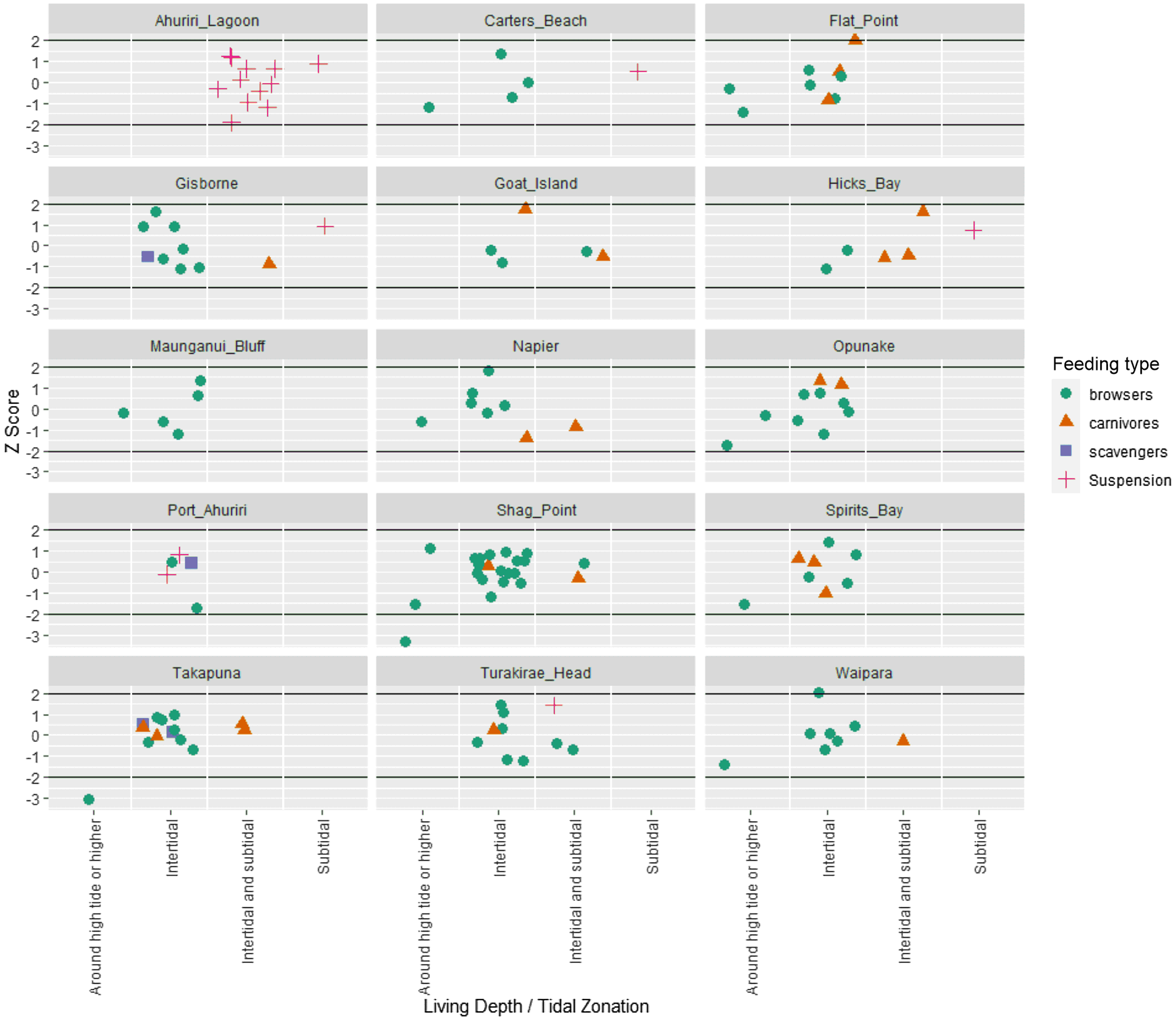
Figure 5 Deviation of individual samples from the location mean for locations with greater than five ΔR measurements. Samples in this figure have symbology categorized by type of feeding and are aligned in columns by their preferred living depth (also known as tidal zonation). The z-score measures how many standard deviations below or above the population mean an individual sample. This plot shows several samples from the “around high tide or higher” category have z scores around 2, i.e., they deviate by two or more standard deviations from the location mean.
-
If there are consistent high or low deviations from the mean for a certain feeding, environment type or tidal zonation, it would suggest that habitat factor is influencing the ΔR20 value preserved in the shell.
-
If there is no correlation between the extreme z-scores and the feeding, living environment or tidal zonation categorisation then the variation from mean cannot be attributed to one of these habitat variables, i.e., habitat factors do not influence ΔR.

For this process, we start with an assumption that each location has the same marine carbon reservoir that each sample draws from. By undertaking intra-location comparison of ΔR and habitat factors, rather than comparing between locations, we can control for localized geological or hydrological factors that may be influencing ΔR because all samples at a specific location will be similarly influenced. Ideally, we would have samples from the same location collected in the same year to tightly control for the same ΔR value in the water due to possible seasonal to local decadal temporal changes in ΔR. However, the available sample set was not large enough to have a reasonable number of samples from the same year at the same location. When locations with <5 samples are removed, 15 locations remained in the dataset. Figure 4 shows the deviation from mean for all samples at each of the 15 locations with ≥5 samples, categorized by feeding type and environment. At every site there is scatter around the mean, but there is no particular feeding type or environment with consistently high or low deviations from the mean. For example, if there were a feeding type that promoted the incorporation of older carbon into shells then the z-score for that feeding type would be consistently more negative than the mean. This is only a useful exercise at locations where multiple feeding and environment types have been sampled. All locations except Ahuriri Lagoon and Maunganui Bluff have more than one feeding type, but over half the locations only sample the open coast, rocky shoreline environment. The locations of Gisborne, Hicks Bay, Takapuna and Port Ahuriri all have multiple feeding types and environments and are most instructive for showing no consistent deviations from the mean for any particular feeding or environment.
The deviation from mean, categorized by feeding type and tidal zonation is shown in Figure 5. As with other variables, tidal zonation does not appear to have a major influence on how far a sample lies from the location mean. In these data there is good spread across the tidal zonation categories because all locations, except Port Ahuriri, have samples from at least two different tidal zonations. The only tidal zonation that shows some consistent deviation below the mean (more negative ΔR values) is the “around high tide or higher” category. There are eight locations with samples from “around high tide or higher” and at 7 of the 8 locations, the samples are below the mean ΔR for that location.
To gauge how significant this deviation from the mean is, we can compare the average z-scores for all categories across feeding, tidal zonation and environment. For this analysis we converted all z-scores to their absolute values so that positive and negative z scores did not average one another out. We see on Figure 6 that the “around high tide or higher” category of tidal zonation has a larger average z-score than all other categories. The mean z-score for “around high tide or higher” is 1.35, meaning most samples from the high tide or higher living depth are around 1.3 standard deviations from the mean ΔR for their location. As shown in Figure 6, the samples from “high tide or higher” have consistently more negative ΔR. The reasons for the lower ΔR in samples from the high tide level may be related to the increased proportion of time the mollusks spend out of marine water. Hogg et al. (Reference Hogg, Higham and Dahm1998) found that open coast intertidal mollusks were enriched in in 14C compared to the subtidal and estuarine zones, they attributed the enrichment to increased aeration due to waves. The same reasoning could hold for the samples in this study: the high tide samples may incorporate a greater proportion of atmospheric carbon in their shells through the time exposed to the atmosphere, their diet, or the marine water aeration due to waves. There are only two species represented in the “around high tide or higher” category: Austrolittorina antipodum and Austrolittorina cincta, both small periwinkles that live on rocky substrates around the high tide mark, they are described as generalist herbivores that feed on lichen, green algae and diatoms. It is possible the negative deviation of high tide specimens is particular to these periwinkle species and other mollusks from the high tide zone could be unaffected by a negative ΔR deviations. Regardless of the reason for the negative deviation of “around high tide or higher” specimens, we exclude them from our analysis of spatial variation in ΔR.
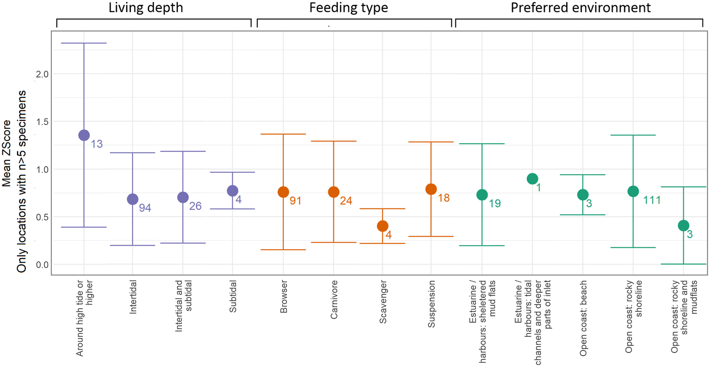
Figure 6 Mean z-score and 1σ range of groups based on living depth, environment or feeding type. This analysis uses the same dataset as Figures 4 and 5 whereby locations with <5 individual samples have been removed. For this plot, the z-scores were converted to absolute values so that positive and negative z scores did not average one another out. The number of individual specimens in each group are shown by the number next to each datapoint. The plot shows the “around high tide or higher” category has a larger value and greater range than all other groupings.
Spatial Variation of ΔR
At the global scale, ΔR varies by latitude with higher latitudes (and zones of coastal upwelling) having larger ΔR values than low latitudes (Alves et al. Reference Alves, Macario, Ascough and Bronk Ramsey2018). This broad relationship does not hold up for the New Zealand coastline, probably due to the relatively small latitudinal spread (34°S to 46°S) or the complexity of the ocean current circulation patterns (Figure 1A, 3). Comparative regional studies of ΔR use water mass characteristics and circulation patterns as the basis for regional subdivisions of ΔR (Ulm Reference Ulm2006; Coulthard et al. Reference Coulthard, Furze, Pieńkowski, Chantel Nixon and England2010; Merino-Campos et al. Reference Merino-Campos, De Pol-Holz, Southon, Latorre and Collado-Fabbri2019). However, the ocean currents, including strong flows through Cook Strait dividing the North and South Island, make it difficult to subdivide New Zealand coastal waters based on water mass characteristics. Rather than arbitrarily subdividing the New Zealand coast into regions based on oceanographic or geographic boundaries and calculating ΔR for each region, we use the approach of grouping locations along the coast based on similarity in ΔR. Stretches of coastline with similar ΔR are grouped together until a point at which the ΔR noticeably changes, and then a new grouping starts.
Prior to this analysis, we combined some locations together if they were very close to one another, for example, Goat Island (two samples), Ti Point (two samples) and Kempt’s Beach (one sample) are within 6 km of one another so are combined into the Goat Island location. Samples from Te Araroa, Ruatoria and Tuparoa were combined into the Hicks Bay locality as they are all within 35 km of one another. Individually, the four sites would not have more than two samples, but collectively the Hicks Bay locality has six samples. Westport (1 sample) is combined with Carters Beach (four samples, 6 km apart) and Orepuki (one sample) is combined with Bluff (two samples, 50 km apart). We removed locations with less than three samples, and we removed samples from the dataset from the “around high tide or higher” environment as we have demonstrated they have a negative ΔR offset. The previously collected offshore fish otolith samples of Higham and Hogg (Reference Higham and Hogg1995) are also excluded because they are not coastal, they were collected from a wide geographic area offshore, with the specific collection locations not recorded.
From the filtered dataset of 163 samples (including 150 from this study and 14 from previous studies), Figure 7 shows a plot of ΔR20 values for each location around the New Zealand coast. The locations are ordered by distance clockwise from the southern-most location of Bluff (noting that Spirits Bay in the north is actually the furthest point from Bluff, locations further clockwise from Spirits Bay get closer to Bluff). Our interpretation of the spatial groupings is shown in the lower plot on Figure 7. We have delineated four groups A–D (Table 2). This grouping of locations is based on a visual assessment of the similarity in mean ΔR20, we then use Kruskal-Wallis test to confirm it is appropriate to group the locations together (further explained below). There are some outlier locations within the geographic area of Group D that are also discussed in greater detail below.

Figure 7 (A) Boxplots of the mean and standard deviation of ΔR20 by location, ordered by distance clockwise around the coastline from Bluff (for locations with n > 3). (B) Same plot as (A) with interpretations of groups based on similarity in mean ΔR. (C) Location names and the geography extent of Groups A–D.
Table 2 Description of Groups A–D, with number of samples used in each group and the mean ΔR20 (1900–1950) for each group (*Group B age range of samples is 1855–1950).

To assess whether it is appropriate to average the ΔR values across Groups A–D we use the Kruskal-Wallis test, a one-way analysis of variance. This is a non-parametric method for testing whether samples originate from the same distribution, i.e., it tests whether the mean ΔR of one location significantly is different to the mean ΔR of another location within the same group. If the mean ΔR of different locations are significantly different from one another then it would not be appropriate to place them in the same group. Figure 8 shows the mean, standard deviation, and distribution of ΔR values across each location within Groups A–D with the results of the Kruskal-Wallis test noted above each. In all cases, the p-value of the Kruskal-Wallis test is >0.05 which is an indicator that the differences between the means of each location within a group are not statistically significantly.
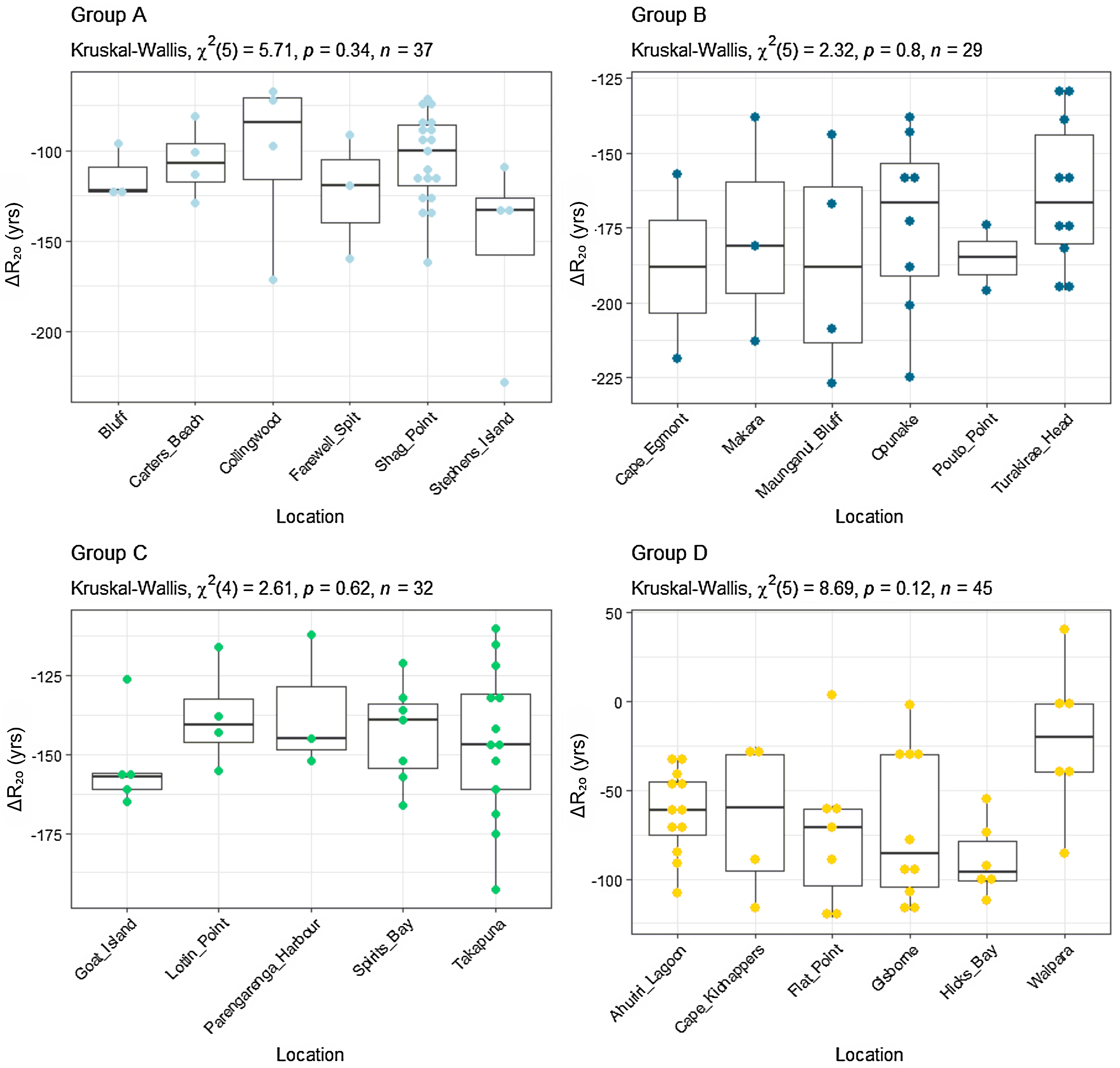
Figure 8 Mean, standard deviation and distribution of ΔR20 within each location within Groups A–D along with the results of the Kruskal-Wallis test. The coloured dots represent individual ΔR values within each location.
In the case of Group D, a number of iterations were tested to refine the samples and locations included in the group that is shown on Figure 8. On an individual sample basis, the only sample removed from Group D was sample NZA69051, a specimen of Cellana flava (limpet) from Waipara with a ΔR20 of 227 ± 18 yr (Figure 7A). This sample was an obvious outlier for the Waipara location (Figure 7B) and is likely to have been a shell that was not collected alive. Our initial collection of locations for Group D included Mahia Peninsula and Turakirae Head, but this group failed Kruskal-Wallis test and the post-hoc Dunn’s Test (a pairwise comparison between each location to identify which locations have statistically different means) identified Mahia Peninsula and Turakirae Head as having different (lower) mean ΔR20 values than the rest of the Group D locations (Figure 7B). Turakirae Head is located within Cook Strait and is closer to Makara (Group B) than other Group D locations (Figure 7C), and it is logical to put Turakirae Head with Group D (noting that its position within Group D in Figure 7B is an artefact of how we calculated distance clockwise from Bluff).
Mahia Peninsula is geographically in the middle of Group D so there is no geographic reason to group this location elsewhere (Figure 7C). The four samples from Mahia Peninsula are tightly clustered around a mean ΔR20 of –138 ± 16 yr, while the mean ΔR20 of Group D without Mahia Peninsula is –70 ± 39—an offset between the location and wider group of ∼70 years (Figure 9B). When Mahia Peninsula is included with other Group D locations (Figure 9B), the Kruskal-Wallis test fails (χ2 (6) = 17.7, p= 0.007, n = 49). The post-hoc Dunn’s Test shows Mahia Peninsula has a statistically significant (p < 0.05) different mean to all other locations within Group D. These analyses suggest Mahia Peninsula should not be included with the rest of the Group D locations. A single sample from Opoutama (15 km west of Table Cape, Mahia Peninsula but on the western side of the peninsula, Figure 9A) has a ΔR20 value of –44 ± 19 yr, this fits within the 1σ range of Group D but does not fit within the range of Mahia Peninsula. Although the Opoutama sample is a single sample from that location, it is further evidence that samples from Mahia Peninsula are anomalously low compared to the coastal waters north and south of the Peninsula. We do not know a specific reason why Mahia Peninsula values are more negative than nearby locations. Plausible reasons for anomalous ΔR values such as hardwater effect due to carbonate rocks (e.g., Petchey and Clark Reference Petchey and Clark2011), or upwelling (e.g., Macario et al. Reference Macario, Alves, Belém, Aguilera, Bertucci, Tenório, Oliveira, Chanca, Carvalho and Souza2018) are not evident at this location and in any case would be expected to cause a positive ΔR effect in any case. A negative ΔR effect could be caused by high freshwater input from large rivers (Alves et al. Reference Alves, Macario, Ascough and Bronk Ramsey2018), but no large rivers discharge near the eastern coast of Mahia Peninsula. The anomalous Mahia Peninsula samples are an indicator that care should be taken when applying ΔR values to locations that have not been directly measured, as variability can and does occur.

Figure 9 (A) Hawke’s Bay region with the extent of limestone in orange (data from Heron Reference Heron2020). Inset map of New Zealand shows the national distribution of limestone. Specific Hawkes Bay locations discussed in the text are also shown, as is the pre-1931 extent of Ahuriri Lagoon. (B) Mean, standard deviation and distribution of ΔR20 within each location within Group D with Mahia Peninsula included. Mahia Peninsula ΔR20 values are generally lower than other locations and this group fails the Kruskal-Wallis test (p < 0.05). (C) Mean, standard deviation and distribution of ΔR20 within each location near Napier with the division between pre-1931 and 1931 collections shown.
The Napier area presents several problems with calculating a ΔR value for the area due to a wide range in ΔR values from within a relatively small geographic area. We have shell collections from two eras in the Napier area: museum specimens collected 1907–1923 (pre-1931 collection), and specimens that we assume died in the 1931 earthquake collected in 2019 (1931 collection). The 1931 collection consists of 11 Ruditapes largillierti and one Dosina mactracea, these are typically found in the current-swept, subtidal entrance channels into harbours. The tight clustering of ages for these samples (Figure 9C) supports the assumption that they all died at the same time, i.e., in the 1931 earthquake. The ΔR20 values for the pre-1931 collection have a broad spread from 414 ± 19 yr to –121 ± 18 yr and the 1931 collection ΔR20 values have a range from –108 ± 18 yr to –32 ± 18 yr (Figure 9C). As discussed in the Methods section, it is difficult to relocate where some of the pre-1931 collection samples came from as the coastal geography of the area changed substantially due to 1.5 m of uplift in the 1931 Napier earthquake. We can infer from the location names that a substantial proportion of the samples came from within the pre-1931 Ahuriri Lagoon or from on the spit separating the lagoon from the open bay. There are two possible reasons for the difference in ΔR values between the pre-1931 and 1931 collections: (1) a substantial number of the pre-1931 collection were not collected alive, or (2) the pre-1931 collection is affected by a carbonate-rich water of the lagoon leading to large offsets in ΔR from the open coast. The first reason is possible but given the collector of most of the pre-1931 Napier samples was W. R. B. Oliver, who also collected many samples from other regions, it would be unusual that in one location a great number of dead specimens were collected. The likelihood that Ahuriri Lagoon specimens are affected by carbonate-rich waters seems more likely when a map of the distribution of limestone around New Zealand is examined (Figure 9A). The coastal region around Napier has a greater area of limestone than any other coastal location of New Zealand. The catchment of streams and rivers that drain into Ahuriri Lagoon are almost entirely limestone, probably causing a hardwater effect (e.g., Petchey and Clark Reference Petchey and Clark2011; Petchey et al. Reference Petchey, Clark, Lindeman, O’Day, Southon, Dabell and Winter2018). The hardwater effect produces older-than-expected ages for marine shells, with consequently higher ΔR20 values, in fact, the highest ΔR20 values around New Zealand come from Ahuriri Lagoon (Figure 7A). The hardwater effect is consistent with the wide range in a ΔR values from the pre-1931 dataset as some species and some environments will be more or less sensitive to the influence of limestone as the mixing of open ocean water, estuarine water and freshwater varies spatially. We considered whether δ13C from the samples could be used to identify local hard water effects (Petchey et al Reference Petchey, Clark, Lindeman, O’Day, Southon, Dabell and Winter2018) but found no relationship between δ13and ΔR for the Ahuriri Lagoon dataset. We contend however that the 1931 collection is a reliable indicator of the open coast marine reservoir value because these species (Ruditapes largillierti and one Dosina mactracea) were living in strong tidal flows, at subtidal depths at the mouth of the lagoon. Their position suggests that they were far from the freshwater inflow points to the lagoon and probably less impacted by the hardwater effect.
DISCUSSION
Our new dataset of 170 ΔR20 values from 31 locations significantly expands the dataset of ΔR values for the New Zealand mainland coast. The new dataset allows a re-evaluation of the appropriate marine reservoir correction values for New Zealand. Previously most research in New Zealand using ΔR has used an average of all mainland ΔR values. Previously the New Zealand-wide mean ΔR20 was calculated at –154 ± 38 yr (Table 1). The average of our new dataset is –94 ± 99 yr. If we combine the pre-2019 and new dataset the resulting average ΔR20 is –100 ± 95 yr. There is a significant shift of ∼50 years between the pre-2019 and new datasets and an increase in the uncertainty. Given this research shows a large spread in ΔR20 values spatially, the increase in uncertainty at a national scale is to be expected and is an appropriate reflection of the variability in marine reservoir values for the New Zealand coastline. However, our increased density in ΔR20 values and our analysis of these data shows that spatial variations in ΔR20 exist and regional ΔR20 values are more appropriate than a national average. Our recommended regional divisions are shown in Figure 7 and the ΔR20(1900–1950) values listed in Table 2. Ultimately it will be up to users of the Marine Reservoir Correction Database to select the spatial coverage of ΔR20 values that best represent the locality they are using a marine calibration for. In some cases, users of the marine reservoir corrections database may choose to use very site-specific ΔR20 values if there are adequate nearby ΔR20 values in the database.
Our recommendation is that our regional ΔR20 values, delineated by Groups A–D are used for calibrations of marine samples from shallow coastal waters, except for samples from (1) the Chatham Islands, (2) Mahia Peninsula, (3) lagoons near Napier:
-
Chatham Islands: We did not obtain new ΔR measurements for the Chatham Islands as they have been covered by datasets presented in Petchey et al. (Reference Petchey, Anderson, Hogg and Zondervan2008a).
-
Eastern coast of Mahia Peninsula: It is not known why Mahia Peninsula has anomalously low ΔR20 values compared to the coastal waters north and south of the Peninsula, but it is an important location in coastal hazard studies due to the exceptionally well-preserved Holocene marine terraces (Berryman et al. Reference Berryman, Clark, Cochran, Beu and Irwin2018). Calibrations for the eastern coast of Mahia Peninsula should use the local ΔR20 value of –138 ± 16 yr rather than the regional ΔR20 value for Group D of –70 ± 39 yr.
-
Lagoons near Napier: ΔR20 values from the pre-1931 sheltered areas of Ahuriri Lagoon have higher and more variable ΔR values than samples collected from the lagoon entrance (Figure 9C). We have suggested the sheltered lagoon samples have been influenced by a hardwater effect produced by the limestone catchment. We recommend open coast marine samples from near Napier are calibrated with the regional ΔR20 value of –70 ± 39 yr. Samples collected from Ahuriri Lagoon, and other lagoons nearby with similar limestone geology could be calibrated with a mean value from the pre-1931 dataset but given the broad range of ΔR values in this dataset it will result in calibrated ages having a very wide age range, potentially rendering them unsuitable for most applications. The Napier area encompasses two important palaeoseismology sites: Ahuriri Lagoon (Hayward et al. Reference Hayward, Grenfell, Sabaa, Carter, Cochran, Lipps, Shane and Morley2006, Reference Hayward, Grenfell, Sabaa, Cochran, Clark, Wallace and Palmer2016), and Pakuratahi Valley (Clark et al. Reference Clark, Howarth, Litchfield, Cochran, Turnbull, Dowling, Howell, Berryman and Wolfe2019). Ahuriri Lagoon has a post-7000 yr BP history of 8 earthquakes that caused coastal subsidence and two that caused coastal uplift. The evidence for these earthquakes is preserved in the alternating intertidal silt and saltmarsh-freshwater peats of the lagoon embayment. About half of the age control for these past earthquakes has been obtained from marine samples. Given the importance of the earthquake record from Ahuriri Lagoon for understanding the frequency of large earthquakes on the Hikurangi subduction zone we recommend the age model for this site is revisited and greater weight placed in terrestrial radiocarbon ages along with the tephrochronology, with marine samples recalibrated and down-weighted, or entirely removed from the earthquake age model. Future work in this area should attempt to only use terrestrial samples and tephra horizons for age control.
Implications for Selection of Radiocarbon Samples from Coastal Hazard Study Sites
Significant effort is usually put toward selecting the best material for radiocarbon dating to obtain the most reliable and precise ages possible, and information from this ΔR dataset can help us better understand what marine material is optimal or sub-optimal for radiocarbon dating. For example, conventional practices have discouraged the selection of gastropods for radiocarbon dating due to potential for older carbon to be incorporated into the shell from their food sources. In New Zealand, previous research has shown estuarine deposit-feeders Macomona liliana and Amphibola crenata produce anomalous 14C concentrations making them unsuitable for radiocarbon dating (Higham and Hogg Reference Higham and Hogg1995; Hogg et al. Reference Hogg, Higham and Dahm1998). There have however, been few attempts to test whether different species, habitats or feeding behaviours affect the 14C content of marine specimens commonly dated in New Zealand coastal environments.
Our dataset shows no significant differences between the mean ΔR values for different categories of feeding method and preferred coastal environment. Previous research suggests the feeding method may produce the most distinct variation in ΔR but a statistically distinct mean ΔR for suspension-feeding mollusks versus other feeding methods is not borne out by our dataset. Previously identified anomalous species of Macomona liliana and Amphibola crenata are not well represented in our dataset so it is hard to re-assess their suitability for radiocarbon dating. One A. crenata specimen from Ahuriri Lagoon yielded a ΔR20 of 336 ± 19 yr, the second highest ΔR value in our dataset. However, given it was collected in Ahuriri Lagoon and is likely influenced by a hardwater effect, it is hard to isolate the cause of the high ΔR value. The δ13C value of this sample is the lowest in our dataset at –2.49‰ (Supplementary Data Table 1), a value consistent with high freshwater input (Petchey et al. Reference Petchey, Clark, Lindeman, O’Day, Southon, Dabell and Winter2018). The very high ΔR value for the A. crenata is in line with the observations noted in Higham and Hogg (Reference Higham and Hogg1995) that A. crenata gives spurious results and we suggest this species should continue to be avoided for radiocarbon dating. No M. liliana were measured in our dataset so we cannot re-examine its suitability for radiocarbon dating.
Our dataset does show that tidal zonation of mollusks can have an influence on ΔR values, but the only category affected are the “around high tide or higher” tidal zonation specimens that have a lower ΔR than other tidal zonation categories. This offset implies specimens from the “high tide or higher” category may produce anomalously young radiocarbon ages compared with their actual age. As noted in the Analysis section, there were only two species dated from this tidal zone: Austrolittorina antipodum and Austrolittorina cincta. The 17 specimens of A. antipodum and A. cincta were obtained from 12 different locations suggesting the anomaly was not swayed by one dominant location. While the low ΔR of the high tide or higher category could be specific to the periwinkles, A. antipodum and A. cincta, our result is consistent with observations by Hogg et al. (Reference Hogg, Higham and Dahm1998) that the open coast intertidal environment was characterized by higher 14C concentrations compared with estuarine and open coast subtidal environments. Out of caution we suggest specimens from high tidal level environments on open, rocky coasts should be avoided for radiocarbon dating. If these specimens are radiocarbon dated due to a lack of other options, we recommend awareness of the likely younger-age-bias of the result. It may be possible to apply a particular marine reservoir correction that accounts for the offset produced by the high tide environment, but our dataset is not large enough to quantify precisely what that offset should be on top of the regional ΔR.
Further Research Needs
The presentation of this ΔR20 dataset for the mainland New Zealand coast is the first step in a process of re-evaluating marine radiocarbon ages around the New Zealand coast. For many samples, and for many areas, the changes arising due to recalibration will be minor, but some areas will see a greater change of several 10s to 100s of years. In particular, it is likely the increased uncertainties on ΔR will broaden the 95% range of calibrated marine radiocarbon ages, resulting in lower precision but reflective of the real variability in ΔR around New Zealand’s coasts. However, there remain some aspects of understanding the New Zealand marine reservoir correction that are poorly resolved, these are (i) spatial gaps, and (ii) understanding temporal variation.
With regard to spatial gaps, the combined pre-2019 dataset and our new dataset still does not adequately cover some areas of the mainland New Zealand coast (Figure 3). The Bay of Plenty coastline (including Coromandel Peninsula) and the West Coast/Fiordland region of the South Island do not have any coverage. The Bay of Plenty region should be able to be rectified by analysis of more museum samples as there is coverage of this area in the NMNZ collection. It was an oversight of this study not to collect samples from this region because we initially assumed it was covered by the fish otoliths in the Higham and Hogg (Reference Higham and Hogg1995) study. Our closer interrogation of this revealed the fish otolith samples had been incorrectly located in the Marine Reservoir Corrections Database. The West Coast and Fiordland regions may be more problematic because there are few samples in the NMNZ collection from these areas. Previous Fiordland data by Hinojosa et al. (Reference Hinojosa, Moy, Prior, Eglinton, McIntyre, Stirling and Wilson2015) were in the Marine Reservoir Corrections Database but have now been withdrawn, highlighting the difficulty in obtaining reliable samples for this area. The eastern Marlborough and Kaikōura coastal areas still remain a gap in spatial coverage of ΔR, which is problematic as several coastal paleoseismology studies from this region have direct relevance to understanding seismic hazards in the Cook Strait area, including the capital city, Wellington (e.g., Pizer et al. Reference Pizer, Clark, Howarth, Garrett, Wang, Rhoades and Woodroffe2021; Howell and Clark Reference Howell and Clark2022). The Kaikōura coastal region is a location of occasional ocean upwelling (Chiswell and Scheil Reference Chiswell and Schiel2001), and 14C-depleted upwelled waters may potentially cause anomalously old radiocarbon ages (e.g., Soares and Dias Reference Soares and Dias2006). Obtaining ΔR values for the Kaikōura area is a priority for understanding if marine radiocarbon ages from this region are affected by an upwelling signal.
The other significant region with little to no ΔR data is the offshore realm of New Zealand. Significant palaeoclimate and palaeoseismology records have been and continue to be obtained from high-resolution analysis of deep-sea sediment cores (e.g., Sikes et al. Reference Sikes, Howard, Neil and Volkman2002; Barnes et al. Reference Barnes, Bostock, Neil, Strachan and Gosling2013; Pouderoux et al. Reference Pouderoux, Proust and Lamarche2014; Bostock et al. Reference Bostock, Hayward, Neil, Sabaa and Scott2015). In many cases, core chronology since the last glacial period is underpinned by radiocarbon ages on planktic foraminifera. In the northern parts of New Zealand, tephra horizons provide additional isochrons but these can have issues relating to identification and reworking (e.g., Hopkins et al. Reference Hopkins, Wysoczanski, Orpin, Howarth, Strachan, Lunenburg, McKeown, Ganguly, Twort and Camp2020; Pizer et al. Reference Pizer, Howarth, Clark, Wilson, Tickle, Hopkins and Dahl2023). Understanding if ΔR differs between offshore and coastal waters is important for understanding whether our coastal ΔR values should be applied offshore but there are few constraints on ΔR in the offshore realm (Hitt et al. Reference Hitt, Sinclair, Neil, Fallon, Komugabe-Dixson, Fernandez, Sutton and Hellstrom2022). It is possible to derive an offshore ΔR value if a high density of radiocarbon ages is collected around the primary tephra deposits of eruptions with ages constrained by onshore terrestrial radiocarbon ages (e.g., Pizer et al. Reference Pizer, Howarth, Clark, Wilson, Tickle, Hopkins and Dahl2023), but few studies collect the required density of radiocarbon ages around tephras to obtain an offshore ΔR in this manner.
A further aspect of ΔR in New Zealand that needs investigation is the question of temporal change in ΔR through time. Petchey and Schmid (Reference Petchey and Schmid2020) have studied temporal change in ΔR around New Zealand from paired marine/terrestrial radiocarbon ages from archaeological sites that span the past 800 years. Their study indicates there is temporal change in ΔR associated with climate shifts, but for coastal hazard research the timeline >800 years needs further investigation. This is not likely to be possible using the paired marine/terrestrial method from archaeological sites because the sites do not extend older than ∼800 yr BP in New Zealand. Hitt et al. (Reference Hitt, Sinclair, Neil, Fallon, Komugabe-Dixson, Fernandez, Sutton and Hellstrom2022) have documented changes temporal changes of ∼150 14C years in ΔR over the past 3000 years from paired radiocarbon and U/Th ages on black coral from two sites offshore to the northeast of New Zealand and a further promising avenue is paired marine radiocarbon ages and tephra deposits in offshore sediment cores. There is a rich archive of sediment cores from along the east coast of the North Island that may provide the requisite combination of tephra horizons and foraminifera, but as discussed above, determination if or how offshore and coastal ΔR values differ would be critical.
CONCLUSIONS
Accurate dating of Holocene coastal hazard events such as earthquakes and tsunamis typically hinges upon marine radiocarbon ages. As the precision of radiocarbon dating and our ability to use many dates for event age modelling has improved in the past decade, we are increasingly seeing the need for a more refined understanding of the marine reservoir correction for New Zealand. The existing dataset has not been supplemented since 2008, aside from the contribution of Clark et al. (Reference Clark, Howarth, Litchfield, Cochran, Turnbull, Dowling, Howell, Berryman and Wolfe2019). In this study we have added 170 new samples to the marine reservoir correction dataset for New Zealand (including the Clark et al. Reference Clark, Howarth, Litchfield, Cochran, Turnbull, Dowling, Howell, Berryman and Wolfe2019, samples). Our expanded dataset of ΔR20(1900–1950) values for the mainland New Zealand coast allows a re-evaluation of the most appropriate marine reservoir correction for marine radiocarbon ages. From our dataset we have evaluated the influence of location, feeding method, tidal zonation and environmental preference on the variance in ΔR values around the New Zealand coast. We find the variability in ΔR is best explained by spatial factors. We recommend the subdivision of New Zealand into four regions, each with a different ΔR20 value ranging from –171 ± 29 to –70 ± 39 yr. Some local exceptions to the regional subdivision of the New Zealand mainland coast were identified, namely the eastern coast of Mahia Peninsula and the limestone-bedrock dominated lagoons near Napier. The cause of the anomaly at Mahia Peninsula is unknown but the limestone catchments of Ahuriri Lagoon are a likely cause of a hardwater effect in coastal lagoons near Napier.
We found that habitat and feeding-related factors produce no statistically significant differences in ΔR values when specimens from the same location are compared. Of note, we found no significant differences between ΔR values from suspension-feeding organisms compared with browsers, scavengers, and carnivores. The only exception we found in terms of habitat, was that specimens living at high tide level or above on rocky open coasts appear to produce a lower ΔR than mollusks living at lower tidal levels, potentially resulting in anomalously young radiocarbon for species form this environment.
Future research will involve using this much-expanded ΔR20 dataset to recalibrate marine radiocarbon ages from along the Hikurangi Subduction Zone and from other key coastal hazard study sites across New Zealand. This will allow a re-evaluation as to how coastal uplift, subsidence and paleotsunamis are temporally correlated along the Hikurangi Subduction Zone, with likely implications for the size and frequency of large to great subduction earthquakes.
SUPPLEMENTARY MATERIAL
Table of ΔR20 values including details of collection location, collection year, ΔR20, species, and environmental and habitat characteristics. Environmental and habitat characteristics assigned with reference to Morton and Miller (Reference Morton and Miller1973). Dataset column refers to new (this study) and old (pre-2019 ΔR samples from the New Zealand mainland coast in the global marine reservoir database. Table presented as a csv file. To view supplementary material for this article, please visit https://doi.org/10.1017/RDC.2023.120
ACKNOWLEDGMENTS
We would like to thank the staff of the Rafter Radiocarbon Laboratory, particular Jenny Dahl and Margaret Norris for their support of this project, and Nicola Litchfield for her review of this manuscript. We acknowledge the National Museum of New Zealand Te Papa Tongarewa for access to the national collection of mollusks. We also thank Bruce Hayward for his advice on sampling mollusks killed by the 1931 Napier earthquake. This project was funding primarily by Toka Tū Ake Earthquake Commission (EQC Biennial Grant, Project 20789), with additional support from New Zealand Ministry of Business, Innovation and Employment (MBIE) through the Global Change through Time and Te Riu-a-Māui Zealandia programme (Strategic Science Investment Fund, contract C05X1702).


 Open access