
Abstract
Linear genetic programming (LGP) is a genetic programming paradigm based on a linear sequence of instructions being executed. An LGP individual can be decoded into a directed acyclic graph. The graph intuitively reflects the primitives and their connection. However, existing studies on LGP miss an important aspect when seeing LGP individuals as graphs, that is, the reverse transformation from graph to LGP genotype. Such reverse transformation is an essential step if one wants to use other graph-based techniques and applications with LGP. Transforming graphs into LGP genotypes is nontrivial since graph information normally does not convey register information, a crucial element in LGP individuals. Here we investigate the effectiveness of four possible transformation methods based on different graph information including frequency of graph primitives, adjacency matrices, adjacency lists, and LGP instructions for sub-graphs. For each transformation method, we design a corresponding graph-based genetic operator to explicitly transform LGP parent’s instructions to graph information, then to the instructions of offspring resulting from breeding on graphs. We hypothesize that the effectiveness of the graph-based operators in evolution reflects the effectiveness of different graph-to-LGP genotype transformations. We conduct the investigation by a case study that applies LGP to design heuristics for dynamic scheduling problems. The results show that highlighting graph information improves LGP average performance for solving dynamic scheduling problems. This shows that reversely transforming graphs into LGP instructions based on adjacency lists is an effective way to maintain both primitive frequency and topological structures of graphs.
1 Introduction
Linear genetic programming (LGP) is an important member of the family of genetic programming and has shown a competent performance [1]. An LGP individual is a sequence of instructions that manipulate a set of registers. The LGP individual executes the instructions sequentially to represent a computer program [2,3,4]. LGP has undergone considerable development and has been successfully applied to classification [5,6,7], symbolic regression [8, 9], combinatorial optimization [10, 11], control tasks [12], and other real-world problems [13, 14].
One of the most salient features of LGP is its graph characteristics. By connecting primitives based on registers, an LGP individual can be decoded into a directed acyclic graph (DAG). Primitives are the basic functions and terminals that compose GP programs. Presenting LGP individuals (i.e., programs) by DAGs has different advantages from a raw genotype (i.e., a sequence of register-based instructions). Graphs represent programs in a more compact representation. On the other hand, a raw genotype enables neutral search in program spaces and memorizes potential building blocks [15, 16]. Empirical studies verified that graphs and LGP genotypes are competitive for different tasks [17, 18]. Therefore, it is valuable to take advantage of both representations.
There are some studies about utilizing graph information in the course of LGP evolution, but they did not fully investigate the LGP graph characteristics. More specifically, the utilization of graphs in LGP is one-way (i.e., the existing LGP studies mainly consider DAGs as a compact and intuitive way to depict the programs). Whether there is an effective way to bridge graphs (i.e., phenotype) and LGP instructions (i.e., genotype) is unknown yet. The absence of an effective transformation from DAGs to instructions precludes LGP from fully utilizing the graph information and cooperating with other graph-related techniques such as neural networks. To have a better understanding of LGP graph-based characteristics, a two-way transformation between graphs and LGP programs is necessary.
To bridge graphs to LGP, the overall goal of this paper is to design a graph-to-instruction transformation for LGP individuals to accept the graph information of DAGs in evolution. The main challenge lies in the fact that DAGs do not contain register information, but LGP individuals are register-based instruction sequences. This paper proposes two strategies to address the register issue in a graph-to-instruction transformation. In the first transformation strategy, LGP individuals accept graph information without considering the topological information that is represented by registers. We assume that if topological information is not that important, ignoring the register identification is a simple and effective way to convey graph information. In the second strategy, LGP individuals identify the registers (by guessing) for the instructions to reconstruct topological information. However, it is hard to perfectly reconstruct the topological structures by registers because of the absence of register information in DAGs. To this end, we aim to answer the following research questions: (1) what necessary information is needed for DAGs in the graph-to-instruction transformation, (2) how to identify the registers based on graphs, and (3) how effective are the aforementioned two transformation strategies.
To answer the above research questions, this paper first develops new genetic operators based on graph node frequency, adjacency matrix, and adjacency list, to fulfill the two transformation strategies. To keep the transformation from a graph to a program intuitive, we treat the two parents in LGP crossover operators as two graphs and exchange their search information via the graph information. We assume that the two LGP programs are able to effectively share knowledge if these graph-based genetic operators effectively convey graph information (e.g., building blocks). Second, we conduct a case study on dynamic scheduling problems, specifically, dynamic job shop scheduling (DJSS) problems, to verify the effectiveness of the proposed genetic operators. The experimental results demonstrate that making better use of graph information enhances LGP performance and that the adjacency list is the recommended graph information to bridge DAG to instructions in LGP.
2 Literature review
2.1 Linear genetic programming genotype
Every LGP individual \(\textbf{f}\) is a sequence of register-based instructions \(\textbf{f}=[f_0,f_1,\ldots ,f_{l-1}],l\in [l_{min},l_{max}]\), where l is the number of instructions, and \(l_{min}\) and \(l_{max}\) are the minimum and maximum number of instructions respectively. Every instruction f has three parts: destination register \(R_{f,d}\), function \(fun_f(\cdot )\), and source registers \(R_{f,s}\). All of the destination and source registers come from the same set of registers \({\mathcal {R}}\). Note that constants (e.g., input features) in LGP programs are seen as a kind of read-only registers, which only serve as source registers. An instruction reads the values from source registers, performs the calculation indicated by the function, and writes the calculation results to the destination registers. Re-writable registers are known as calculation registers. In every program execution, the registers are first initialized by certain values such as “1.0”, and the instructions are executed one by one, from \(f_0\) to \(f_{l-1}\), to represent a complete computer program. The final output of the computer program is stored in a pre-defined output register, which is normally set to the first register by default.
However, not all instructions contribute to the final output. When an instruction is not connected with the program body producing the final output, or the instruction can be removed without affecting the program behavior, the instruction becomes ineffective in calculating the final output. The ineffective instructions are also called “introns”. Contrarily, the instructions that participate in the calculation of the final output are defined as effective instructions, which are also called “exons”. Specifically, the term “intron” in this paper mainly denotes the structural intron whose destination register is not used as source registers by the following instructions.Footnote 1 Introns and exons can be identified by an algorithm that reversely checks each instruction in the program based on the output registers [4].
Figure 1 shows an example of the genotype of an LGP program and its corresponding phenotype in DAG. Specifically, there are eighteen instructions in the program, but only eleven of the instructions are effective (i.e., exons). The introns are highlighted in grey, following a double slash. The final output is returned by the first register \(\text {R}[0]\). All of the instructions manipulate a register set \({\mathcal {R}}\) with eight registers. There are eight input features (i.e., constant registers), denoted \(\text {Input}[0]\) to \(\text {Input}[7]\). The eight registers are initialized by the eight input features respectively at the beginning of every execution.

An LGP program example and its corresponding DAG. “Input\([\cdot ]\)” are read-only registers, and “R\([\cdot ]\)” are calculation registers
A number of studies have been carried out to extend the linear representation in LGP. For example, Hu et al. [19,20,21] analyzed the relationship between LGP genotype and its evolvability. Heywood et al. [22] proposed a page-based LGP to group instructions into different pages. Oliveira et al. [23] designed problem-specific chromosome representation for LGP to solve software repair (i.e., genetic improvement). These existing studies show the potential of linear representations and their distinct behaviors compared to tree-based GP (TGP) programs. Having a better understanding of LGP is beneficial to analyze GP methods from a different perspective.
2.2 Evolutionary framework of LGP
The evolutionary framework of LGP in this paper is the generational evolutionary framework (i.e., selecting parents for breeding and accepting offspring without further selection), which is the recommended framework for the case study on dynamic scheduling problems [24]. Note that it is different from the recommended evolutionary framework of LGP (i.e., steady-state evolutionary framework—a portion of the least fit individuals in the population are replaced with offspring at each iteration) for solving classification and symbolic regression problems [4, 17, 25].

The schematic diagram of LGP genetic operators
LGP breeds offspring by a series of genetic operators for every generation. There are three basic genetic operators in basic LGP (i.e., crossover, macro mutation, and micro mutation) as shown in Fig. 2. Specifically, crossover produces new programs by swapping instruction segments between their instruction sequences [26]. Macro mutation produces offspring by removing a random instruction from the program or inserting a new instruction into a random position of the program [27]. Micro mutation produces offspring by replacing primitives, including functions and registers, but not changing the total number of instructions. These three genetic operators are triggered based on pre-defined probabilities. The LGP genetic operators have undergone good development. For example, Downey et al. [28] proposed a class graph crossover to evolve LGP programs for multi-class classification. The class graph crossover produces offspring by swapping the instructions that contribute to the same output register (i.e., the same sub-class in multi-class classification). Besides, various problem-specific genetic operators are developed to address specific applications respectively [22, 23]. However, the existing genetic operators of LGP are all designed based on LGP genotype (i.e., instruction sequence) and cannot truly accept graphs as genetic materials.
2.3 Graphs in linear genetic programming
An LGP program can be represented as a DAG. The instruction sequence is transformed into a DAG by connecting functions and constants of exons based on the registers [4] (i.e., connecting “\(+\)” to “\(\times\)” in DAG if “\(+\)” uses the register overwritten by “\(\times\)” as one of its inputs, see instruction 16 and instruction 13 in Fig. 1). As shown in the right part of Fig. 1, the last instruction of the LGP program that overwrites the output register (instruction 17 in this example) is seen as the start node in the DAG. Since the source registers of instruction 17 store the results of instructions 15 and 16 respectively, the start node has two outgoing edges, directing to two graph nodes (“−” and “\(+\)”) respectively. The indices along the edges indicate the first and second inputs for “\(\max (\cdot )\)”.
Evolving LGP programs based on graphs has some benefits over evolving LGP programs based on instruction sequences. First, graphs allow us to have more precise control over the variation step size of exons. Contrarily, the variation in raw genotype might lead to an unexpectedly large variation step size since it might deactivate and activate different sub-programs. Second, swapping LGP building blocks based on graphs protects the useful building blocks from being destructed [29]. For instance, when we swap the instruction sub-sequences of two LGP programs to produce offspring, the exons (and introns) in the sub-sequences are not guaranteed to be effective (and ineffective) after swapping since they might be deactivated (or activated) in the new LGP program context. The building blocks in the sub-sequences might be distorted severely, which often leads to destructive variations (i.e., the fitness of the offspring is worse than the fitness of the parents) [30]. But swapping sub-graphs of LGP parents naturally maintains the connections of primitives within sub-graphs and protects effective building blocks from being deactivated. Third, treating LGP programs as graphs can further evolve the program by replacing the introns into effective building blocks, especially when the instruction sequence reaches the maximum program size. Fully utilizing the maximum program size implies a longer effective program length and a better search performance [15, 31]. Last but not least, explicitly considering graph information in LGP programs encourages LGP to have a more compact representation and reduce redundancy.
Nevertheless, explicitly employing graphs in LGP has not been well investigated though it is an effective way to show the program. Brameier and Banzhaf [4] claimed that using graph representations to evolve LGP program does not always lead to better performance than conventional LGP in solving classification and symbolic regression problems, but evolving graph representations needs much more complicated genetic operators than imperative representation. However, the discussion in [4] does not show implementation details of the compared methods. Sotto et al. [17, 25] compared a number of graph-based GP methods, including LGP, in their experiment. However, the graph-based genetic operators of the compared graph-based GP methods in [17, 25] mainly manipulate genotype by graph-based mutations and miss graph-based crossover which produces new graphs by swapping sub-graphs. The absence of graph-based crossover limits the variation step of graph-based GP methods and precludes useful building blocks from being shared among the population. Huang et al. [29] proposed two graph-based genetic operators, including graph-based crossover and mutation, and tested their effectiveness on combinatorial optimization problems. Their results imply the potential of the graph-based crossover. But the crossover is designed based on LGP genotype rather than graphs, and the graph-based mutation is not effective.
In short, the explicit use of graphs in LGP has not been well investigated from the following aspects: (1) the existing literature misses the graph-based crossover that truly swaps sub-graphs to produce offspring; (2) the existing literature misses the graph-to-instruction transformation.
2.4 Relationship among graphs, exons, and LGP instructions
First, fully utilizing graph characteristics of LGP is different from only evolving exons. Graphs are the phenotype of LGP programs, and LGP instructions are the genotype. Exons in LGP instructions are the instructions that are highly related to the graphs since the graphs are decoded based on the exons. However, exons cannot fully stand for the phenotype since graphs carry the essential information of both imperative primitives and their connection, which is a higher-level representation than the exons, while exons are highly dependent on the context of an LGP program. Besides, a graph is an abstract representation that is free from specific genotype design (e.g., register-based instructions in LGP or Cartesian coordinates in Cartesian GP). Representing GP programs by graphs enables GP methods to analyze building blocks effectively and to exchange genetic materials with many other graph-based techniques.
Second, evolving LGP programs based on graphs cannot replace evolving LGP based on instruction sequences. Some existing studies have proposed to directly represent GP programs by graphs and to evolve GP programs by manipulating the graphs [17, 18, 32]. However, their results show that different GP representations are suitable to different tasks. For example, LGP and Cartesian GP have certain advantages in solving the tested digital circuit design problems because of the limited reuse on intermediate results while TGP is good at solving the tested symbolic regression problems [17, 18]. Evolving programs by genotype instead of graphs also enables LGP and Cartesian GP individuals to perform neutral search (i.e., varying the genotype of an individual but not changing the fitness value) and retain potential building blocks in the individuals [15, 16, 33, 34]. The neutral search and the potential building blocks have been shown to be helpful for LGP and Cartesian GP programs to jump out of local optima and improve the population diversity in a wide range of problems. Further, existing literature on evolving GP programs by graphs directly only considered node and edge mutation on graphs in producing offspring and missed graph-based crossover, which makes these methods inefficient to exchange useful building blocks.
In a nutshell, a graph is an abstract representation of effective LGP instructions, while a sequence of LGP instructions represents underlying codes that include both effective and ineffective instructions. Graphs enable LGP programs to cooperate with other graph-based techniques and explicitly take the topological structures into consideration, while instruction representations enable the neutral search and the memory of potential building blocks. Finding an effective way to bridge these two representations would be useful for LGP evolution. However, to the best of our knowledge, there is no existing literature of graph-based genetic programming investigating suitable ways of utilizing the general graph information (e.g., adjacency list) and effective transformations from graph to LGP instructions. The graphs of LGP programs are not fully utilized yet.
2.5 Other DAG-based genetic programming
There are some other graph-based genetic programming methods besides LGP. For example, Cartesian genetic programming [35] is one of the well-known graph-based genetic programming methods. The genotype of Cartesian GP is a list of grid nodes. Each node specifies a function, its connections with other nodes, and its Cartesian coordinate in the grid. By executing these grid nodes based on the connection, the individuals of Cartesian GP can be decoded into DAGs to represent computer programs or digital circuits (i.e., the phenotype). Cartesian GP has shown some superior performance in designing digital circuits [36, 37], performing image classification [38], and neural architecture search [39]. Wilson et al. [40] compared Cartesian GP with LGP and found that the way of restricting the interconnectivity of nodes is the key difference between these two graph-based genetic programming methods. Based on the idea of Cartesian GP, Atkinson et al. [18] proposed the Graph Programming method to evolve graphs (abbr. EGGP). Different from Cartesian GP which strictly requires that the connections must go from the right columns to the left columns (i.e., the levels-back constraint), EGGP allows a graph node \({\mathcal {A}}\) to connect any other graph node \({\mathcal {B}}\) in the graph, as long as \({\mathcal {A}}\) and \({\mathcal {B}}\) do not form a cycle in the graph. The EGGP individuals have higher flexibility in topological structures than the LGP and Cartesian GP individuals. They further validated the effectiveness of EGGP on the test problems by comparing it with TGP, Cartesian GP, and LGP [17, 25]. The results show that all the three DAG-based GP methods (i.e., LGP, Cartesian GP, and EGGP) have a great advantage over TGP in searching multiple-output computer programs such as digital circuits. However, these studies have not investigated the graph-based crossover operators that truly swap sub-graphs and the graph-to-instruction transformations.
3 The proposed graph-based genetic operators
The schematic diagram of conveying graph information to LGP instructions is shown in Fig. 3. To investigate the effectiveness of different graph-to-instruction transformation methods, we explicitly transform LGP instruction segments into DAGs [4], and graph-based genetic operators accept the DAGs as genetic materials to produce offspring. The dashed arrow with a question mark is the to-be-investigated step in this paper. We assume that graph-based genetic operators should effectively evolve LGP programs if the graph representation is effective in conveying building block information. To have a comprehensive investigation of the effective transformation from graphs to LGP programs, this paper designs three crossover operators to convey three different types of graph information (i.e., primitive frequency, adjacency matrix, and adjacency list) from graph to LGP instructions. These three crossover operators are frequency-based crossover (FX), adjacency matrix-based crossover (AMX), and adjacency list-based crossover (ALX). Specifically, FX and AMX follow the first graph-to-instruction transformation strategy that bypasses the register identification, and ALX resolves the register identification by a newly proposed register assignment method.

The schematic diagram of accepting graphs as LGP genetic materials. The program-to-DAG transformation (i.e., grey solid arrows) is fulfilled by [4]. The DAG-to-program transformation (i.e., dashed arrow) with a question mark is the focus of this paper
3.1 Frequency-based crossover (FX)
The frequency of primitives is a simple high-level feature of a graph. The frequency of primitives implies the importance of different primitives. Frequency has been widely applied in GP to identify important features [41, 42]. In the FX operator, we utilize the primitive frequency in LGP crossover by seeing the primitive frequency as a kind of distribution.
FX accepts two parent individuals and produces one offspring. The offspring is produced by varying one of the primitives in an instruction of the first parent. When varying the primitive, the old primitive is replaced by a new one based on the frequency of the primitives in the second parent. We hope that varying the primitive based on the frequency of another individual stimulates more useful building blocks. The pseudo-code of FX is shown in Algorithm 1.Footnote 2 The frequency vector is defined as \(\textbf{F}=[fun_1,fun_2,\ldots ,fun_g, in_1, in_2,\ldots ,in_h]\) where g is the number of functions and h is the number of input features. The function \(fun_f\) is sampled by a roulette wheel selection on the function frequency (i.e., \(\textbf{F}[fun_1,fun_2,\ldots ,fun_g]\)). A higher frequency implies a larger probability to be selected. If varying constant is triggered (i.e., \(\texttt {rand}(0,1)<\theta _{fun}+\theta _{con}\) in line 8 of Algorithm 1), one of the source registers is replaced by an input feature which is sampled by a roulette wheel selection on the input feature frequency \(\textbf{F}[in_1, in_2,\ldots ,in_h]\). To ensure that every primitive has a small probability of being selected, we add 1.0 on all the elements of \(\textbf{F}\). The destination register \(R_{f',d}\) and the source registers \(R_{f',s}\) of the instruction \(f'\) are sampled uniformly.

Frequency-based crossover
Figure 4 shows an example of producing offspring by FX. First, FX transforms the second parent into a DAG and obtains the frequency of the primitives. Note that the frequency of primitives in a DAG is different from the frequency of primitives in raw effective instructions, as the effective instructions contain register primitives but the DAG does not. Since the DAG merges all the duplicated constants (i.e., input feature \(x_{i(i=0,1,2)}\)) into one graph node, FX treats the incoming degree as the frequency of constant graph nodes. FX normalizes the frequency of primitives and gets the distribution which further biases the variation on the first parent. We can see that the R[2] in the third instruction of Parent 1 is changed to \(x_0\) based on the distribution.

An example of FX operator
3.2 Adjacency matrix-based crossover (AMX)
The adjacency matrix conveys more graph information than the primitive frequency by highlighting the neighboring relationship of graph nodes. The elements in an adjacency matrix are the frequency of a primitive connecting to another primitive in a DAG. We treat the elements in an adjacency matrix as a kind of distribution by normalizing the elements in each row. To this end, we utilize the adjacency matrix in LGP crossover (i.e., AMX).
Similar to FX, AMX accepts two parents and produces one offspring by varying one primitive in one of the instructions. Different from FX, AMX varies functions and constants by a roulette wheel selection based on the adjacency matrix of the graph from the other parent. The pseudo-code of varying a function or constant based on an adjacency matrix is shown in Algorithm 2Footnote 3 where the adjacency matrix is defined as

Since the constants (i.e., input features) have no outgoing edge in the graph, the two blocks of “constant-out” are two zero matrices. \(\textbf{M}\) is further simplified as \([\textbf{M}_{fun}\ \textbf{M}_{in}]\) where \(\textbf{M}_{fun}\) denotes the neighboring relationship from function primitives pointing to function primitives, and \(\textbf{M}_{in}\) denotes the neighboring relationship from function primitives pointing to input features. When varying the function of the \(l^{*}th\) instruction, AMX first finds the function out that points to the to-be-varied function. From the perspective of LGP genotype, it is equivalent to checking the instructions reversely from \(\textbf{f}(l^*-1)\) and finding the instruction whose destination register is accepted as inputs of \(\textbf{f}(l^*)\). Then AMX applies the Roulette-wheel selection on \(\textbf{M}_{fun}\) and samples a new primitive based on out. To ensure that every primitive has a small probability of being selected, we add 1.0 on all the elements of \(\textbf{M}=[\textbf{M}_{fun}\ \textbf{M}_{in}]\) in the Roulette-wheel selection. When varying the constant of an instruction, AMX applies Roulette-wheel selection based on the function of the instruction and \(\textbf{M}_{in}\).
Figure 5 shows an example of producing offspring by AMX operator. AMX gets a distribution based on the adjacency matrix from the second parent and performs variation based on the distribution. In Fig. 5, the “\(\div\)” in the third instruction of the first parent is varied into “\(+\)”.

An example of AMX operator
3.3 Adjacency list-based crossover (ALX)
An adjacency list is a graph representation that conveys the connection among graph nodes. To fully utilize the topological information carried by the adjacency list, we design an adjacency list-based crossover to vary instruction segments in the parent individuals. The adjacency list in this paper is denoted as
where each item \([fun_i,\textbf{B}_i]\) specifies the function \(fun_i\) and the list of its neighboring graph nodes \(\textbf{B}_i\). Based on the adjacency list, this section proposes ALX.

Transforming an adjacency list to an instruction sequence

RegisterAssignment
ALX accepts two parent individuals (one as recipient and the other as donor) to produce one offspring. Rather than swapping the instruction sequences like basic linear crossover [26], the donor parent first selects a sub-graph from the DAG (by selecting a sub-sequence of instructions) and obtains the corresponding adjacency list \(\textbf{L}\). The recipient accepts the adjacency list and constructs the new instruction sequence based on the adjacency list. The newly constructed instruction sequence is used to replace another sub-sequence of instructions in the recipient. The pseudo-code of transforming an adjacency list into an instruction sequence is shown in Algorithm 3. First, ALX selects a crossover point from the recipient parent and removes a sub-sequence of instructions from the recipient. Based on the adjacency list, ALX randomly generates a sequence of instructions. Specifically, the functions in the newly generated instructions are coincident with the adjacency list. Since the adjacency list does not convey the information of registers, we propose a register assignment method for ALX to identify the registers in those newly generated instructions, as shown in Algorithm 4.

An example of ALX operator. The selected graph nodes, the newly generated instructions, and the newly updated primitives are highlighted in gray color
In general, Algorithm 4 checks the instruction sequence reversely based on the adjacency list to assign the registers in all the new instructions. There are two main steps in Algorithm 4, assigning destination registers and assigning source registers. From the perspective of topological structures, assigning destination registers is equivalent to providing the results of the sub-graph to the upper part of the DAG, while assigning the source registers is equivalent to taking the results from the lower part of the DAG as the inputs of the sub-graph. When assigning destination registers, Algorithm 4 ensures the effectiveness of all the newly generated instructions. On the other hand, Algorithm 4 assigns source registers based on the neighboring graph nodes (i.e., functions or constants) specified by the adjacency list. Specifically, if the neighboring graph node is a function, Algorithm 4 collects the possible instructions whose functions are coincident with the neighboring function in the adjacency list and randomly assigns the destination register from one of the possible instructions as the source register.
Figure 6 shows an example of producing an offspring by ALX. First, ALX selects a sub-graph from the second parent, consisting of “\(-,\times ,+\)”, and gets the corresponding adjacency list. Then ALX generates a new instruction segment based on the adjacency list and swaps it into the first parent (i.e., the 2nd to 4th instructions in the new instruction sequence). To maintain the topological structures among newly inserted instructions, ALX applies the register assignment method (i.e., Algorithm 4) to update the registers. Algorithm 4 replaces the destination register of the 4th instruction to R[1] to ensure the three swapped-in instructions are effective. Then, based on the adjacency list, Algorithm 4 update the source registers in the three swapped-in instructions so that “−” accepts the results from “\(\times\)” and “\(\times\)” accepts the results from “\(+\)” and the constant \(x_0\). We can see that “\(-,\times ,+\)” are connected together, and the 2nd and 4th instructions manipulate suggested constants by the adjacency list in the offspring.
3.4 Summary
We summarize the pros and cons of different graph information representations, as shown in Table 1. Transforming graphs into LGP instructions based on graph node frequency and adjacency matrix is a good alternative solution to bypass the puzzle of identifying registers for new instructions. However, frequency-based and adjacency matrix-based information do not explicitly consider the topological information, which might be susceptible to the number of registers (i.e., graph width). Besides, adjacency matrices of LGP graphs might be often too sparse to effectively guide the search. Adjacency list can convey graph node frequency and their topological structures simultaneously but is dependent on a register assignment method to reconstruct the topological structures. The effectiveness of the register assignment method might limit the effectiveness of adjacency list information. To verify the effectiveness of different representations of graph information, we compare to an existing graph information sharing method that swaps effective instructions. Swapping effective instruction has shown its effectiveness in solving DJSS [29]. However, it cannot fulfill the DAG-to-program transformation since it only manipulates LGP programs.
4 A case study on dynamic job shop scheduling
To verify the effectiveness of different transformation methods from DAG to LGP genotype, this paper applies LGP to solve dynamic job shop scheduling (DJSS) problems [43,44,45]. Many GP variants such as TGP, basic LGP, and LGP with graph-based crossover [29], have shown their performance in solving DJSS problems. It is straightforward to verify the effectiveness of the proposed graph-based genetic operators with other GP variants based on DJSS problems. Besides, DJSS is a challenging combinatorial optimization problem that can be seen in many real-world production scenarios. Investigating the effectiveness of the proposed genetic operators on DJSS problems is beneficial for GP in practice.
Different from the static job shop scheduling problems whose information is known beforehand, DJSS problems have different types of dynamic events which will occur during the process of the job shop. The information of these dynamic events cannot be known until they occur. There have been many studies successfully using GP methods to learn scheduling heuristics for DJSS problems [46, 47]. In this paper, we set up the simulator based on the model of DJSS problems and see the simulation performance as the fitness of GP individuals.
4.1 Problem description
This paper focuses on DJSS with new job arrival. The job shop in our DJSS problems processes a set of jobs \({\mathbb {J}}=\{{\mathcal {J}}_1,\cdots ,{\mathcal {J}}_{|{\mathbb {J}}|}\}\). Each \({\mathcal {J}}_j\) consists of a sequence of operations \({\mathbb {O}}_j=\left[ {\mathcal {O}}_{j1},\cdots ,{\mathcal {O}}_{jm_j}\right]\) where \(m_j\) is the total number of operations in \({\mathcal {J}}_j\). Each job \({\mathcal {J}}_j\) arrives to the job shop at the time \(\alpha ({\mathcal {J}}_j)\) with a weight of \(\omega ({\mathcal {J}}_j)\), and the information of \({\mathcal {J}}_j\) cannot be known until their arrival. The jobs are processed by a set of machines \({\mathbb {M}}=\{{\mathcal {M}}_1,\cdots ,{\mathcal {M}}_{|{\mathbb {M}}|}\}\). Specifically, each operation \({\mathcal {O}}_{ji}\) of \({\mathcal {J}}_j\) is processed by a specific machine \(\pi ({\mathcal {O}}_{ji})\) with a positive processing time \(p({\mathcal {O}}_{ji})\). Each machine has a queue to store the available operations and at most processes one operation at any time. When an operation is finished, the machine selects an available operation from the queue. The major task in the DJSS problems of this paper is to prioritize the available operations in each machine queue so that the job shop can effectively react on the new arrival jobs. We adopt three different optimization objectives in this paper, as listed as follows, where \(T_{max}\) denotes the maximum tardiness among all the jobs, \(T_{mean}\) and \(WT_{mean}\) denote the mean and weighted mean tardiness over the job set \({\mathbb {J}}\) respectively, and \(c({\mathcal {J}}_j)\) and \(d({\mathcal {J}}_j)\) denote the completion time and the due date of job \({\mathcal {J}}_j\) respectively.
4.2 Design of comparison
To investigate the effectiveness of different graph-to-instruction transformation methods, we design seven compared methods. The first two methods are the basic TGP [48] and LGP [4] which are seen as the baseline. The third to fifth methods respectively verify the three newly designed graph-based genetic operators. We replace the micro mutation of the basic LGP with FX and AMX in the third and fourth compared methods respectively because the variation step sizes of FX and AMX are similar to LGP micro mutation (i.e., only varying one or a few primitives in the parent but not changing the total number of instructions). The third and fourth methods are denoted as LGP + FX and LGP + AMX respectively. The fifth compared method is denoted as LGP + ALX, in which the linear crossover in the basic LGP is replaced by ALX. The other settings in LGP + FX, LGP + AMX, and LGP + ALX are kept the same as the basic LGP. To comprehensively investigate the effectiveness of transforming graph information into instruction sequences, we further compare the LGP with an existing graph-based crossover [29] denoted as LGP + GC, which has shown encouraging performance gain from LGP crossover in solving DJSS problems. Finally, we investigate the effectiveness of the cooperation of multiple graph-based genetic operators. Since our prior investigation shows that LGP + FX has better average performance than LGP + AMX, we replace the micro mutation and linear crossover in the basic LGP with FX and ALX simultaneously. The LGP with FX and ALX is denoted as LGP + FA.
The parameters of all the compared methods are shown in Table 2. Since the prior investigation [49] has shown that the basic TGP and LGP are effective under different settings of population size and the number of generations, we set these two parameters to the best values for the TGP and LGP-based methods respectively. The parameters of the genetic operators are defined based on [29, 49]. All the compared methods start the search from a small initial program size. All the LGP methods manipulate a register set with 8 registers. The elitism rate and the tournament size of all the compared methods are defined as top 1% and 7 respectively. All the compared methods adopt the same function set \(\{+,-,\times ,\div ,\max ,\min \}\) and terminal set, as shown in Table 3.
It is noted that to improve the generalization ability of GP methods, DJSS training instances in different generations have different simulation seeds [24]. For each generation, we use elitism selection to retain the best-so-far individuals for the next population (i.e., reproduction) and apply tournament selection to select parents for breeding. The newly generated individuals and the best-so-far individuals form the next population.
4.3 Simulation settings
The effectiveness of the compared methods is verified by the simulation of DJSS problems. Specifically, the job shop has 10 machines. All the jobs come into the job shop based on a Poisson distribution. The arrival rate of the jobs is defined by the utilization level \(\rho\), which is a parameter of the Poisson distribution [29]:
where \(\nu\) and \(\upsilon\) are the average number of operations of the jobs and the average processing time of the operations respectively. The expected processing time of the jobs decreases with the increment on \(\rho\). Each job contains 2 to 10 operations, and each operation is processed by a different machine with a processing time ranging from 1 to 99 time units. The due date of a job \(d_i\) is defined by multiplying a due date factor of 1.5 with the total processing time of job i (i.e., summing up the processing time of all the operations). The weights of jobs are set as 1, 2, and 4 for 20, 60, and 20% of all the jobs, respectively.
Each GP individual is decoded into a dispatching rule that prioritizes the available operations in each machine queue. We see the performance of the overall simulation as the performance of the GP individual. To evaluate GP individuals in a steady-state job shop, the simulation is warmed up with the first 1000 jobs and takes the following 5000 jobs into account to evaluate its performance.
To investigate all the compared methods comprehensively, six DJSS scenarios are set up based on the existing literature [29, 49, 50]. Specifically, two utilization levels are defined (i.e., 0.85 and 0.95). A higher utilization level implies a busier job shop in which bottlenecks are more likely to occur. The scenarios are denoted by “\(\langle \text {Objective},\text {utilization level}\rangle\)” based on the three optimization objectives mentioned in Sect. 4.1 and the two utilization levels (i.e., \(\langle T_{max},0.85\rangle\), \(\langle T_{max},0.95\rangle\), \(\langle T_{mean},0.85\rangle\), \(\langle T_{mean},0.95\rangle\), \(\langle WT_{mean},0.85\rangle\), and \(\langle WT_{mean},0.95\rangle\)). These six scenarios cover a wide range of objectives (including the worst case (\(T_{max}\)) and mean performance) and utilization levels. Each scenario evaluates a GP method by 50 independent runs. For each independent run, the GP method searches a dispatching rule based on the training DJSS instances, one DJSS instance per generation, and tests the performance of the dispatching rule on 50 unseen DJSS instances. Each DJSS instance is a simulation with 6000 jobs. The performance of the 50 unseen DJSS instances is aggregated as the test performance for a certain independent run.
5 Empirical results
5.1 Test performance
The mean test performance of all the compared methods in solving the six DJSS scenarios is shown in Table 4. We conduct a Friedman test with a significant level of 0.05 on the test performance of all the compared methods. The p value of the Friedman test is 0.016 which implies there is a significant difference among the compared methods. The notation “\(+\)”, “−”, and “\(\approx\)” in Table 4 denote a method is significantly better than, significantly worse than, or statistically similar to the basic LGP based on Wilcoxon rank-sum test with a significant level of 0.05. The best mean values are highlighted in bold.
As shown in Table 4, first, all the three newly proposed graph-based genetic operators, together with LGP + GC, improve the overall performance of basic LGP since the mean ranks of most LGP methods (except LGP + AMX) with graph-based genetic operators are better than basic LGP (i.e., smaller is better). Second, the performance of LGP is improved with the amount of graph information overall. Specifically, LGP + FX and LGP + AMX (i.e., distribution and local topological structures) have worse mean ranks than LGP + ALX (i.e., topological structures of sub-graphs), and LGP + ALX has a worse mean rank than LGP + GC which conveys topological structures and register information in exchanging genetic materials. LGP + FA which conveys more graph information by using multiple graph-based genetic operators has the same mean rank as LGP + GC. Table 4 also shows that the best mean test performance is mainly achieved by LGP + ALX, LGP + GC, and LGP + FA, which verifies that conveying more graph information (e.g., primitive frequency and topological structures) in the course of exchanging genetic materials is effective in improving LGP performance. It is noted that although the adjacency matrix is supposed to convey more graph information than graph node frequency, the adjacency matrix does not help LGP + AMX perform better than LGP + FX since adjacency matrices of LGP graphs are often too sparse to provide search bias (i.e., most elements in the adjacency matrix are zero which degenerates AMX to uniform variation). In short, all the three newly proposed graph-based genetic operators have very competitive performance with basic LGP, which implies the proposed graph-based genetic operators effectively convey the graph information from one parent individual to the other. The improvement in mean ranks implies the potential of utilizing graph information.
5.2 Training convergence
This section compares the training performance of different graph-based genetic operators, as shown in Fig. 7. Specifically, we compare the test performance of the best individuals from all the compared methods at every generation. Overall, all compared methods perform quite similarly in most problems. But in some problems, we can see gaps among the curves. For example, LGP + FA converges faster than the others in \(\langle Tmax,0.85 \rangle\) and \(\langle Tmax,0.95 \rangle\), and LGP + GC converges faster than the others in \(\langle WTmean,0.95 \rangle\) in the first 20,000 simulations. Further, if we look at the lowest convergence curves at different stages, we find that LGP + ALX, LGP + GC, and LGP + FA alternatively take the leading positions in training. For example, in \(\langle Tmean, 0.85 \rangle\), LGP + ALX is slightly lower than the others in most simulations but is caught up by LGP + GC from 20,000 to 40,000 simulations. Based on the results, we confirm that conveying as much graph information as possible (e.g., LGP + ALX, LGP + GC, and LGP + FA) can improve LGP performance to some extent.

The convergence of different graph-based genetic operators
To conclude, the proposed graph-based genetic operators successfully carry the information from LGP instructions to graph and back to instructions since the training and test performance of the proposed graph-based genetic operators are similar to or better than the performance of conventional genetic operators that directly exchange instructions. We also see that the performance gain of graph-based genetic operators increases with the amount of graph information overall. Furthermore, if we look back at the pros and cons of the graph information (Table 1), we find that (1) bypassing the issue of identifying registers (i.e., LGP + FX and LGP + AMX) is a feasible way to transform graphs to instructions, but it is not as effective as LGP + ALX because of the loss of graph information (2) LGP + ALX performs as competitively as swapping effective instructions directly, which implies that the register assignment method in LGP+ALX reconstructs the topological structures quite well without much deterioration on effectiveness.
6 Further analyses
6.1 Effectiveness on different graph shapes
To comprehensively investigate the effectiveness of the proposed graph-based genetic operators in different graphs, this section compares the graph-based genetic operators on different graph shapes. The graph shape in LGP (i.e., depth and width of a graph) is approximately defined by the maximum number of instructions (i.e., depth) and the maximum number of registers (i.e., width). A graph shape is denoted by “\(\langle \# ins, \# reg \rangle\)” in this paper, specifying the maximum depth and width of the graph. This section tests nine different graph shapes, from a shallow and narrow graph to a deep and wide graph. The nine graph shapes are \(\langle 25ins, 4reg \rangle\), \(\langle 25ins, 8reg \rangle\), \(\langle 25ins, 12reg \rangle\), \(\langle 50ins, 4reg \rangle\), \(\langle 50ins, 8reg \rangle\), \(\langle 50ins, 12reg \rangle\), \(\langle 100ins, 4reg \rangle\), \(\langle 100ins, 8reg \rangle\), and \(\langle 100ins, 12reg \rangle\). Figure 8 shows the mean rank of the compared methods obtained by a Friedman test on all the six DJSS scenarios in each graph shape. The compared methods include basic LGP, and LGP with four graph-based genetic operators (i.e., LGP + FX, LGP + AMX, LGP + ALX, and LGP + GC) to separately investigate the effectiveness. We apply the Bonferroni–Dunn’s test as a post-hoc analysis on the mean rank of the compared methods to detect the significant difference with the control algorithm (We take the algorithm with the best mean rank as the control algorithm). The shadow in Fig. 8 denotes the threshold of the critical difference of Bonferroni–Dunn’s test with a significance level of 0.05. The critical difference of the Bonferroni–Dunn’s test is 2.28 [51]. The threshold value equals to the critical difference plus the mean rank of the control algorithm (e.g., the threshold is \(2.28+2=4.28\) in \(\langle 25ins, 4reg \rangle\)). If the mean rank of a compared algorithm is larger than the threshold value, the compared algorithm is significantly worse than the control algorithm. Otherwise, the compared algorithm performs statistically similarly to the control algorithm.

The mean rank of the compared methods on all the six DJSS scenarios in different graph shapes. The shadows denote the threshold of the critical difference of Bonferroni–Dunn’s test with a significance level of 0.05
First, Fig. 8 shows that when the graph is shallow (i.e., 25 instructions), LGP + ALX and LGP + GC have better (i.e., smaller) overall mean ranks than (or have at least similar mean rank to) the other compared LGP methods in the three graph widths. It implies that LGP + ALX and LGP + GC can fully utilize the maximum program size to construct effective solutions. In contrast, basic LGP, LGP + FX, and LGP + AMX have worse mean ranks than LGP + ALX and LGP + GC because they cannot effectively turn introns into useful building blocks and have insufficient space to contain effective solutions (i.e., under-representing [52]). Note that when graphs have abundant space to contain effective solutions (i.e., growing from 25 instructions to 100 instructions), the building blocks stored in introns improve the diversity of genetic materials [53] and improve the performance of the basic LGP and LGP + FX (i.e., smaller mean ranks).
Second, when the graph width grows from 4 to 12 registers, we see a salient improvement (i.e., become smaller) in the mean ranks of LGP + ALX and LGP + GC. For example, the mean ranks of LGP + ALX and LGP + GC reduce from about 3.4 in \(\langle 50ins, 4reg \rangle\), to about 2.0 in \(\langle 50ins, 8reg \rangle\) and \(\langle 50ins, 12reg \rangle\). The other LGP methods (i.e., basic LGP, LGP + FX, and LGP + AMX) that apply linear crossover to swap genetic materials have a slightly better mean rank than LGP + ALX and LGP + GC on long and narrow graphs (i.e., \(\langle 50ins, 4reg \rangle\) and \(\langle 100ins, 4reg \rangle\)) since swapping instruction segments directly is equivalent to exchanging sub-graphs when there are few introns. However, the mean ranks of basic LGP, LGP + FX, and LGP + AMX constantly increase with the graph width in all the graph depths. Specifically, the overall performance of LGP + FX and LGP + AMX is significantly worse than LGP + GC on \(\langle 25ins,12reg \rangle\), and the overall performance of basic LGP is significantly worse than LGP + GC on \(\langle 50ins,12reg \rangle\). The results verify that LGP without explicitly maintaining the topological structure is susceptible to the number of registers and is not good at evolving wide graphs.
Third, LGP + ALX has a quite similar performance to LGP + GC in all the nine graph shapes. Given that LGP + ALX maintains the topological structures based on the proposed register assignment method (i.e., Algorithm 4) while LGP + GC directly swap effective instructions, the proposed register assignment method can reconstruct the topological structures in offspring very well.
In short, the mean rank comparison verifies that LGP + ALX and LGP + GC perform averagely better than the other algorithms and are less susceptible to graph width. Besides, the newly proposed register assignment method can effectively reconstruct the topological structures based on the adjacency list. Based on the results, we confirm that ALX is an effective method to transform graphs into LGP instructions.
6.2 Component analyses on ALX
The results in Sect. 6.1 verify that ALX is an effective method for LGP to accept graph information. To investigate the reasons of the superior performance, this section conducts an ablation study on ALX. Given that an adjacency list can convey two kinds of graph information, the frequency of graph nodes and their topological connection, we verify the effectiveness of different graph information separately by four ALX-based methods. We use basic LGP and LGP + ALX as the baseline methods in this section. We develop “ALX/noRegAss” in which we remove the \(\texttt {RegisterAssignment}(\cdot )\) from LGP + ALX. In this case, LGP + ALX generates the instruction segment only based on each item of the adjacency list and does not further connect these generated instructions by registers. The newly generated instruction segment has a similar graph node frequency to the adjacency list but has very different topological structures, and the effectiveness of the instruction segment cannot be ensured (i.e., might contain a lot of introns after swapping into a parent). Besides, we develop “ALX/randSrc” in which we do not assign source registers for the newly generated instruction in ALX (i.e., removing lines 5–15 in Algorithm 4 but ensuring that each newly generated instructions are effective in the offspring). By comparing with ALX/noRegAss, ALX/randSrc eliminates the performance bias caused by the epistases of instructions (i.e., to-be-swapped graph nodes are likely not connected with the parent graph in ALX/noRegAss). Nevertheless, ALX/randSrc does not maintain the topological structures based on the adjacency list either. Note that since all of the parameters in the compared methods follow the settings of the basic LGP which does not maintain the topological structures in its evolution, the compared methods with different components do not show significant performance discrepancy in our prior investigation. Therefore, to highlight the performance discrepancy, we also compare the four compared methods with 12 registers. Other parameters in this section are set the same as Sect. 4.2.
Table 5 shows the results of the compared methods. We apply Friedman test and Wilcoxon test to analyze the test performance of the compared methods. The p values of the Friedman test are 0.284 and 0.012 for 8 and 12 registers respectively, which means there is a significant difference in the test performance with 12 registers. In the comparison with 8 registers, the p values from a pair-wise Friedman test show that all compared methods are similar. However, the mean ranks and the mean test performance of ALX/noRegAss and ALX/randSrc show that only conveying frequency information of graphs is averagely inferior to conveying both frequency and topological information based on adjacency list. The results with 12 registers also show a performance reduction when ALX does not maintain topological structures. The basic LGP and ALX/noRegAss have significantly worse performance than LGP + ALX, and ALX/randSrc has a larger (worse) mean rank and worse mean test performance than LGP + ALX in most scenarios.
In summary, the results confirm that ALX effectively uses both frequency and topological information to improve LGP performance. Specifically, first, graph node frequency improves LGP performance since ALX/noRegAss and ALX/randSrc have better test performance than basic LGP overall. Second, connecting every to-be-swapped graph node with the parent graph (i.e., ALX/randSrc and LGP + ALX) and connecting the newly generated instructions among themselves (i.e., LGP + ALX) both enhance LGP performance.
6.3 Program size and effective ratio
To further understand the behaviors of different graph-based genetic operators, we investigate the mean program length, mean effective program length, and the mean effective ratio of LGP populations in the course of evolution. Specifically, we define the number of (effective) instructions as the (effective) program length and define the effective program length divided by the program length as the effective ratio for a program. We select three scenarios with a utilization level of 0.95 as examples to make analyses. The results are shown in Fig. 9.

The mean program length, mean effective program length, and mean effective ratio of the LGP methods. Y-axis is specified by the first column and X-axis denotes simulations
First, the program length of LGP + ALX and LGP + FA grows more slowly than the others, and all the compared methods finally maintain at a similar level of program length. Given that LGP + ALX and LGP + FA replace conventional linear crossover by ALX, the results imply that ALX has a smaller variation step size than conventional linear crossover and is less suffered from the bloat effect caused by introns. It is because ALX only swaps the effective instructions within an instruction segment (by transforming the effective instructions into a DAG), and the number of effective instructions is often smaller than the length of the instruction segment.
Second, LGP + ALX, LGP + FA, and LGP + GC have larger effective programs than the other compared methods. For example, LGP + ALX and LGP + FA end up with an effective program length of nearly 40 instructions in the three scenarios, while LGP, LGP + FX, and LGP + AMX only maintain at the level of 25 effective instructions. Based on the smaller program length and larger effective program length of LGP + ALX and LGP + FA, it is believed that ALX enables LGP to make better use of program instructions. The higher effective ratios of LGP + ALX and LGP + FA further confirm the conclusion. In terms of effective ratio, LGP + ALX and LGP + FA roughly maintain at the level of 0.8 in the course of evolution, while the other LGP methods without ALX or GC only maintain at the level of 0.55. The full utilization of instructions helps LGP to contain more effective building blocks within a given maximum program size.
7 Conclusions
The main goal of this paper is to find an effective way for LGP to accept graph information during breeding. By investigating four graph-based genetic operators, this paper confirms that the adjacency list is an effective graph representation to transform graphs into LGP instructions in a case study of solving DJSS problems. To address the register assignment issue in graph-to-instruction transformation, this paper proposes a register assignment method. The experimental results show that the register assignment method is effective in reconstructing the topological structures without significant loss of program effectiveness. Note that although we mainly investigate different graph information representations (by corresponding graph-based genetic operators) separately in this paper, LGP can simultaneously utilize more than one kind of graph information during the course of evolution in practice. The experimental results also confirm that fully utilizing different kinds of graph information improves the performance of basic LGP and significantly reduces the susceptibility to maximum graph shapes.
This paper can be seen as a bridge from DAGs to LGP instructions, to make up the missing part of the graph-based theory in existing LGP literature. Further, the proposed graph-based genetic operators in this paper facilitate future cooperation between LGP and many other graph-based techniques and applications, such as neural networks and social network detection. We expect this paper to consolidate the foundation of LGP theory and provide a prior investigation for future LGP studies.
The conclusion in DJSS problems may be generalized to other domains since the proposed graph-to-instruction transformations did not consider the problem-specific features in their design. To verify this point, we plan to extend our experiments to other domains such as regression and classification in future work. Besides, we intend to fully use the graph-based characteristics of LGP to design new techniques, which are rarely taken into account in the existing literature. For example, the intrinsic multiple outputs in LGP can be used in tasks with multiple decisions. The easy reuse of building blocks in LGP can facilitate GP methods to evolve compact programs. We also intend to cooperate LGP with neural networks to perform neural architecture searches.
Availability of data and materials
Non applicable.
Notes
We do not consider semantic introns that is a kind of effective instructions but mainly perform meaningless calculation such as \(x=x+0\), which does not affect the final output.
\(\texttt {rand}(a,b)\) returns a random floating-point number in [a, b). \(\texttt {randint}(a,b)\) returns a random integer number in [a, b]. \(|\cdot |\) denotes the cardinality of a set or a list. \((\cdot )\) following a set or a list denotes getting an element based on the index.
\((x, :)\) and \((:,x)\) following a matrix denote getting the xth row or the xth column of elements respectively.
Algorithm 2 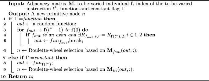
Varying a function or a constant based on the adjacency matrix

References
M. Oltean, C. Grosan, A comparison of several linear genetic programming techniques. Complex Syst. 14, 285–313 (2004)
P. Nordin, A compiling genetic programming system that directly manipulates the machine code. Adv. Genet. Program. 1, 311–331 (1994)
P. Nordin, in Evolutionary Program Induction of Binary Machine Code and Its Applications. Ph.D. Thesis (1997)
M. Brameier, W. Banzhaf, Linear Genetic Programming (Springer, New York, NY, 2007)
M. Brameier, W. Banzhaf, A comparison of linear genetic programming and neural networks in medical data mining. IEEE Trans. Evolut. Comput. 5, 17–26 (2001)
C. Fogelberg, in Linear Genetic Programming for Multi-class Classification Problems. Ph.D. Thesis, Victoria University of Wellington (2005)
S. Provorovs, A. Borisov, Use of linear genetic programming and artificial neural network methods to solve classification task. Comput. Sci. Sci. J. Riga Tech. Univ. 45, 133–139 (2012)
L.F.D.P. Sotto, V.V. Melo, A probabilistic linear genetic programming with stochastic context-free grammar for solving symbolic regression problems, in Proceedings of the Genetic and Evolutionary Computation Conference, pp. 1017–1024 (2017)
Z. Huang, Y. Mei, J. Zhong, Semantic linear genetic programming for symbolic regression. IEEE Trans. Cybern. 1–14 (2022). Early access
L.F.D.P. Sotto, V.V. Melo, M.P. Basgalupp, \(\lambda\)-lgp: an improved version of linear genetic programming evaluated in the ant trail problem. Knowl. Inform. Syst. 52, 445–465 (2017)
Z. Huang, , F. Zhang, Y. Mei, M. Zhang, An investigation of multitask linear genetic programming for dynamic job shop scheduling. in Proceedings of European Conference on Genetic Programming, Cham, pp. 162–178 (2022)
R. Li, B.R. Noack, L. Cordier, J. Borée, F. Harambat, Drag reduction of a car model by linear genetic programming control. Exp. Fluids 58(8), 1–20 (2017)
M. Jamei, I. Ahmadianfar, Prediction of scour depth at piers with debris accumulation effects using linear genetic programming. Mar. Georesour. Geotechnol. 38, 468–479 (2020)
H.V. Arellano, M.M. Rivera, Forward kinematics for 2 DOF planar robot using linear genetic programming. Res. Comput. Sci. 148, 123–133 (2019)
L.F.D.P. Sotto, F. Rothlauf, V.V. Melo, M.P. Basgalupp, An analysis of the influence of noneffective instructions in linear genetic programming. Evolut. Comput. 30, 51–74 (2022)
J.F. Miller, S.L. Smith, Redundancy and computational efficiency in cartesian genetic programming. IEEE Trans. Evolut. Comput. 10, 167–174 (2006)
L.F.D.P. Sotto, P. Kaufmann, T. Atkinson, R. Kalkreuth, M. Porto, M. Basgalupp, Graph representations in genetic programming. Genet. Program. Evol. Mach. 22(4), 607–636 (2021)
T. Atkinson, D. Plump, S. Stepney, Evolving graphs by graph programming, in Proceedings of European Conference on Genetic Programming, pp. 35–51 (2018)
T. Hu, J.L. Payne, W. Banzhaf, J.H. Moore, Robustness, evolvability, and accessibility in linear genetic programming, in Proceedings of European Conference on Genetic Programming, pp. 13–24 (2011)
T. Hu, J.L. Payne, W. Banzhaf, J.H. Moore, Evolutionary dynamics on multiple scales: a quantitative analysis of the interplay between genotype, phenotype, and fitness in linear genetic programming. Genet. Program. Evol. Mach. 13(3), 305–337 (2012)
T. Hu, W. Banzhaf, J.H. Moore, Robustness and evolvability of recombination in linear genetic programming, in Proceedings of European Conference on Genetic Programming, pp. 97–108 (2013)
M.I. Heywood, A.N. Zincir-Heywood, Dynamic page based crossover in linear genetic programming. IEEE Trans. Syst. Man Cybern. Part B Cybern. 32, 380–388 (2002)
V.P.L. Oliveira, E.F. Souza, C.L. Goues, C.G. Camilo-Junior, Improved representation and genetic operators for linear genetic programming for automated program repair. Empir. Softw. Eng. 23, 2980–3006 (2018)
T. Hildebrandt, J. Heger, B. Scholz-reiter, Towards improved dispatching rules for complex shop floor scenarios - a genetic programming approach, in Proceedings of the Annual Conference on Genetic and Evolutionary Computation, pp. 257–264 (2010)
L.F.P. Sotto, P. Kaufmann, T. Atkinson, R. Kalkreuth, M.P. Basgalupp, A study on graph representations for genetic programming, in Proceedings of Genetic and Evolutionary Computation Conference, pp. 931–939 (2020)
W. Banzhaf, P. Nordin, R.E. Keller, F.D. Francone, Genetic Programming: An Introduction on the Automatic Evolution of Computer Programs and Its Applications (Morgan Kaufmann, San Francisco, California, 1998)
W. Banzhaf, M. Brameier, M. Stautner, K. Weinert, Genetic programming and its application in machining technology, in Advances in Computational Intelligence—Theory and Practice, (Springer, Berlin 2003), pp. 194–242
C. Downey, M. Zhang, W.N. Browne, New crossover operators in linear genetic programming for multiclass object classification, in Proceedings of the Annual Genetic and Evolutionary Computation Conference, pp. 885–892 (2010)
Z. Huang, Y. Mei, F. Zhang, M. Zhang, Graph-based linear genetic programming: a case study of dynamic scheduling, in Proceedings of the Genetic and Evolutionary Computation Conference, New York, NY, USA, pp. 955–963 (2022)
P. Nordin, F. Francone, W. Banzhaf, Explicitly defined introns and destructive crossover in genetic programming, in Advances in Genetic Programming, (MIT Press, Cambridge, 1996), pp. 111–134
L.F.D.P. Sotto, F. Rothlauf, On the role of non-effective code in linear genetic programming, in Proceedings of the Genetic and Evolutionary Computation Conference, (ACM, New York, 2019), pp. 1075–1083
E. Medvet, A. Bartoli, Evolutionary optimization of graphs with graphea, in Proceedings of International Conference of the Italian Association for Artificial Intelligence, pp. 83–98 (2020)
A.J. Turner, J.F. Miller, Neutral genetic drift: an investigation using cartesian genetic programming. Genet. Program. Evol. Mach. 16, 531–558 (2015)
B.W. Goldman, W.F. Punch, Analysis of cartesian genetic programming’s evolutionary mechanisms. IEEE Trans. Evolut. Comput. 19, 359–373 (2015)
J.F. Miller, An empirical study of the efficiency of learning Boolean functions using a Cartesian Genetic Programming approach, in Proceedings of the Genetic and Evolutionary Computation Conference, pp. 1135–1142 (1999)
J.F. Miller, D. Job, V.K. Vassilev, Principles in the evolutionary design of digital circuits-part I. Genet. Program. Evol. Mach. 1(1), 7–35 (2000)
J.F. Miller, D. Job, V.K. Vassilev, Principles in the evolutionary design of digital circuits-part II. Genet. Program. Evol. Mach. 1(3), 259–288 (2000)
P.C.D. Paris, E.C. Pedrino, M.C. Nicoletti, Automatic learning of image filters using Cartesian genetic programming. Integr. Comput. Aided Eng. 22(2), 135–151 (2015)
J.F. Miller, D.G. Wilson, S. Cussat-Blanc, Evolving developmental programs that build neural networks for solving multiple problems, in Genetic Programming Theory and Practice XVI. Genetic and Evolutionary Computation. (Springer, Cham, 2019), pp. 137–178
G.Wilson, W. Banzhaf, A comparison of cartesian genetic programming and linear genetic programming, in Proceedings of European Conference on Genetic Programming, pp. 182–193 (2008)
F. Zhang, Y. Mei, S. Nguyen, M. Zhang, Genetic programming with adaptive search based on the frequency of features for dynamic flexible job shop scheduling, in Proceedings of European Conference on Evolutionary Computation in Combinatorial Optimization, pp. 214–230 (2020)
Z. Huang, J. Zhong, L. Feng, Y. Mei, W. Cai, A fast parallel genetic programming framework with adaptively weighted primitives for symbolic regression. Soft Comput. 24, 7523–7539 (2020)
E.K. Burke, M.R. Hyde, G. Kendall, G. Ochoa, E. Ozcan, J.R. Woodward, in A Classification of Hyper-Heuristic Approaches, (Springer, Cham, 2010), pp. 449–468
J. Zhang, G. Ding, Y. Zou, S. Qin, J. Fu, Review of job shop scheduling research and its new perspectives under industry 4.0. J. Intell. Manuf. 30, 1809–1830 (2019)
J. Mohan, K. Lanka, A.N. Rao, A review of dynamic job shop scheduling techniques. Proc. Manuf. 30, 34–39 (2019)
S. Nguyen, Y. Mei, M. Zhang, Genetic programming for production scheduling: a survey with a unified framework. Complex Intell. Syst. 3, 41–66 (2017)
F. Zhang, S. Nguyen, Y. Mei, M. Zhang, Genetic Programming for Production Scheduling (Springer, Singapore, 2021)
J.R. Koza, Genetic programming as a means for programming computers by natural selection. Stat. Comput. 4(2), 87–112 (1994)
Z. Huang, Y. Mei, M. Zhang, Investigation of linear genetic programming for dynamic job shop scheduling, in Proceedings of IEEE Symposium Series on Computational Intelligence, (IEEE, Orlando, FL, 2021), pp. 1–8
Y. Mei, S. Nguyen, M. Zhang, Evolving time-invariant dispatching rules in job shop scheduling with genetic programming, in Proceedings of European Conference on Genetic Programming, pp. 147–163 (2017)
S. García, A. Fernández, J. Luengo, F. Herrera, A study of statistical techniques and performance measures for genetics-based machine learning: Accuracy and interpretability. Soft Comput. 13, 959–977 (2009)
F. Rothlauf, D.E. Goldberg, Redundant representations in evolutionary computation. Evolut. Comput. 11, 381–415 (2003)
T. Hu, W. Banzhaf, Neutrality, robustness, and evolvability in genetic programming, in Genetic Programming Theory and Practice XIV, (Springer, Cham, 2018), pp. 101–117
Acknowledgements
Non applicable.
Funding
Open Access funding enabled and organized by CAUL and its Member Institutions. This work is supported by the Marsden Fund of New Zealand Government under Contract MFP-VUW1913 and Contract VUW1614; in part by the Science for Technological Innovation Challenge Fund under Grant 2019-S7-CRS; and in part by the MBIE SSIF Fund under Contract VUW RTVU1914. The work of Zhixing Huang was supported by the China Scholarship Council (CSC)/Victoria University Scholarship.
Author information
Authors and Affiliations
Contributions
All authors discussed the idea of this paper many times. Specifically, ZH did the experiments and results analyses, and this process repeats a number of times based on discussions. Finally, ZH wrote the first draft, and then all authors discussed and revised this paper with substantial improvements.
Corresponding author
Ethics declarations
Ethical approval
Non applicable.
Additional information
Publisher's Note
Springer Nature remains neutral with regard to jurisdictional claims in published maps and institutional affiliations.
Rights and permissions
Open Access This article is licensed under a Creative Commons Attribution 4.0 International License, which permits use, sharing, adaptation, distribution and reproduction in any medium or format, as long as you give appropriate credit to the original author(s) and the source, provide a link to the Creative Commons licence, and indicate if changes were made. The images or other third party material in this article are included in the article's Creative Commons licence, unless indicated otherwise in a credit line to the material. If material is not included in the article's Creative Commons licence and your intended use is not permitted by statutory regulation or exceeds the permitted use, you will need to obtain permission directly from the copyright holder. To view a copy of this licence, visit http://creativecommons.org/licenses/by/4.0/.
About this article

Cite this article
Huang, Z., Mei, Y., Zhang, F. et al. Bridging directed acyclic graphs to linear representations in linear genetic programming: a case study of dynamic scheduling. Genet Program Evolvable Mach 25, 5 (2024). https://doi.org/10.1007/s10710-023-09478-8
Received:
Revised:
Accepted:
Published:
DOI: https://doi.org/10.1007/s10710-023-09478-8