

Abstract
Entanglement asymmetry is a novel quantity that, using entanglement methods, measures how much a symmetry is broken in a part of an extended quantum system. So far, it has only been used to characterise the breaking of continuous Abelian symmetries. In this paper, we extend the concept to cyclic  groups. As an application, we consider the XY spin chain, in which the ground state spontaneously breaks the
  spin parity symmetry in the ferromagnetic phase. We thoroughly investigate the non-equilibrium dynamics of this symmetry after a global quantum quench, generalising known results for the standard order parameter.
Export citation and abstract BibTeX RIS

Original content from this work may be used under the terms of the Creative Commons Attribution 4.0 license. Any further distribution of this work must maintain attribution to the author(s) and the title of the work, journal citation and DOI.
1. Introduction
In the last few years, the interplay between entanglement and symmetries has become the centre of intense research activity, yielding up a more refined vision of the behaviour of many-body quantum systems [1–6] and creating a new framework to study entanglement [7–21]. For example, novel quantities, such as the symmetry-resolved entanglement entropy [7–9], have been conceived to analyse how entanglement is distributed in the symmetry sectors of a theory. On the other hand, the idea of using entanglement tools to study symmetry breaking has recently arisen. To this end, entanglement asymmetry was proposed in [22] as a measure of how much a symmetry is broken in a part of an extended quantum system. So far, the entanglement asymmetry has been applied to examine the time evolution of an initially broken U(1) symmetry after a quench with a Hamiltonian that preserves it, both in free [22, 23] and interacting integrable systems [24]. In general, it is expected that the symmetry is dynamically restored in a subsystem after the quench. However, unexpectedly, the entanglement asymmetry reveals that the symmetry can be restored earlier when it is initially more broken [22]. This surprising phenomenon can be seen as a quantum version of the very counter-intuitive Mpemba effect: the more a system is initially out of equilibrium, the faster it relaxes. Entanglement asymmetry was also employed in [23] to analyse the special case in which symmetry is not restored and the subsystem relaxes to a non-Abelian generalised Gibbs ensemble (GGE).
The previous works are restricted to the continuous U(1) group. The goal of the present manuscript is to extend the study of the entanglement asymmetry to finite, discrete cyclic  groups. In particular, we consider the
  spin flip parity symmetry of the XY spin chain which, in the thermodynamic limit, is spontaneously broken by the ground state in the ferromagnetic phase [25]. Usually, this symmetry breaking is detected using the one-site longitudinal magnetisation as an order parameter. This order parameter presents the inconvenience that, despite a non-zero value indicating that the symmetry is broken, the converse is not always true [26]. On the contrary, the entanglement asymmetry unambiguously determines whether the symmetry is respected or not. Moreover, although for a single spin the order parameter can be used to measure symmetry breaking, for larger subsystems there are longer range correlations that can break the symmetry and are only taken into account by the entanglement asymmetry. Using this, we study the non-equilibrium time evolution of the
  spin parity symmetry after a global quantum quench in the XY spin chain Hamiltonian, extending the study performed in [27–29] employing the order parameter. Global quenches in this system have been studied from many perspectives; see e.g. [30–44]. We distinguish between chains with open and periodic boundary conditions (OBC and PBC), since the approach to calculate the entanglement asymmetry and the results obtained differ: while in the periodic case this
  symmetry is always restored, the same does not always occur in the open chain due to the presence of boundary modes. Moreover, in the periodic case, by comparing with the analytic results obtained in [27, 28] for the order parameter in the thermodynamic limit, we conjecture an effective expression that describes the evolution of the entanglement asymmetry after the quench.
The paper is organised as follows: in section 2, we define the entanglement asymmetry, we review its main known features for the U(1) group and we extend it to cyclic  groups, describing some of its principal properties in this case. In section 3, we introduce the XY spin chain and we present the behaviour of the entanglement asymmetry of the spin parity in the ground state. Section 4 is devoted to calculating and discussing the entanglement asymmetry after a quantum quench of the XY spin chain with OBC, while in section 5 we carry out a similar analysis but using PBC. In section 6, we draw our conclusions. The manuscript also includes several appendices that describe in detail the more technical points of the main text.
2. Entanglement asymmetry
Let us consider an extended quantum system that can be divided into two spatial parts A and B. If we assume that the total system is in a pure state  , then the state of one of the regions, for example A, is described by the reduced density matrix
  , which is generally a mixed state. We further consider a local charge operator Q given by the sum of the charge in A and B,
  . We assume that Q generates an Abelian group with elements of the form
  , where α is a real number. This includes the unitary group U(1) or the cyclic groups
  .
.
It is well known that, when  respects the symmetry associated with Q, i.e. it is an eigenstate of Q, the reduced density matrix of any subsystem A displays a block-diagonal structure in the eigenbasis of QA
, and the blocks correspond to the sectors of a given charge. In this case, the entanglement entropy of subsystem A can be decomposed into the contributions of each charge sector, known as symmetry-resolved entanglement entropies [7–9].
respects the symmetry associated with Q, i.e. it is an eigenstate of Q, the reduced density matrix of any subsystem A displays a block-diagonal structure in the eigenbasis of QA
, and the blocks correspond to the sectors of a given charge. In this case, the entanglement entropy of subsystem A can be decomposed into the contributions of each charge sector, known as symmetry-resolved entanglement entropies [7–9].
In the case of symmetry-breaking states, entanglement entropy can be used to quantify how much the symmetry generated by Q is broken in a subsystem. In fact, if the state  locally breaks the symmetry in the region A, then ρA
does not commute with QA
. This means that, in the eigenbasis of QA
, ρA
presents non-zero entries outside the sectors of fixed charged
locally breaks the symmetry in the region A, then ρA
does not commute with QA
. This means that, in the eigenbasis of QA
, ρA
presents non-zero entries outside the sectors of fixed charged  ,
,

Download figure:
Standard image High-resolution image here represented by  . From this state, it is always possible to define another density matrix
  that respects the symmetry, i.e.
 ![$[\rho_{A, Q}, Q_A] = 0$](https://content.cld.iop.org/journals/1742-5468/2024/2/023101/revision1/jstatad138fieqn18.gif) . If we take the projection of ρA
on the different charge sectors of QA
and we sum them all, we obtain a block diagonal matrix
. If we take the projection of ρA
on the different charge sectors of QA
and we sum them all, we obtain a block diagonal matrix

Download figure:
Standard image High-resolution image where  is the projector on the subspace of eigenvalue qj
. The density matrix
is the projector on the subspace of eigenvalue qj
. The density matrix  can be physically interpreted as the result of performing a non-selective measurement of QA
in ρA
. From ρA
and its projection
can be physically interpreted as the result of performing a non-selective measurement of QA
in ρA
. From ρA
and its projection  , we can define the entanglement asymmetry [22]

in terms of their von Neumann entropies

The entanglement asymmetry measures how much the symmetry generated by Q is broken in the subsystem A. In fact,  satisfies two crucial properties: it is always non-negative,
  , and it vanishes if and only if
 ![$[\rho_A, Q_A] = 0$](https://content.cld.iop.org/journals/1742-5468/2024/2/023101/revision1/jstatad138fieqn24.gif) [45]. These properties are satisfied whether the total system is in a pure or mixed state. Therefore, the entanglement asymmetry can also be applied to the study of symmetry breaking in mixed states and, in particular, to a system at a certain temperature.
[45]. These properties are satisfied whether the total system is in a pure or mixed state. Therefore, the entanglement asymmetry can also be applied to the study of symmetry breaking in mixed states and, in particular, to a system at a certain temperature.
Since the direct calculation of the von Neumann entropy is normally a difficult task, the usual strategy [46, 47] is to replace it in equation (1) by the Rényi entropies

Then we define the Rényi entanglement asymmetry as

Note that, if we take in this expression the limit n → 1, we recover equation (1). Moreover, Rényi entanglement asymmetries are also non-negative quantities,  , and they cancel if and only if the symmetry is respected in subsystem A, i.e.
 ![$[\rho_A, Q_A] = 0$](https://content.cld.iop.org/journals/1742-5468/2024/2/023101/revision1/jstatad138fieqn26.gif) [48]. It is also important to remark that the Rényi entanglement asymmetries for an integer
[48]. It is also important to remark that the Rényi entanglement asymmetries for an integer  are experimentally measurable in ion traps through randomised measurements [49–53].
2.1. Review of entanglement asymmetry for the U(1) group
In the literature, the entanglement asymmetry has only been analysed for the Abelian unitary group U(1). In this case, the paradigmatic example to understand how it works is the tilted ferromagnetic state,

For θ ≠ 0, this state breaks the U(1) symmetry corresponding to rotations around the z axis, which are generated by the transverse magnetisation  . It has been shown that, if the subsystem A is an interval of contiguous spins of length
  , the entanglement asymmetry behaves as [22]

for large  . To better understand this result, let us focus on the n = 2 Rényi asymmetry
  . Using the Fourier representation of the projectors
  , the projected matrix
  can be written as

Since  is a separable state,
  , and
, and  is the restriction of
  to
to  contiguous spins. We can see equation (7) as the state of A after applying a random element of the U(1) group to ρA
with a uniform probability density. Consequently,
contiguous spins. We can see equation (7) as the state of A after applying a random element of the U(1) group to ρA
with a uniform probability density. Consequently,  can be interpreted as the quantum information loss of the subsystem A after such an operation. Despite the infinite number of elements in the U(1) group, this information loss is finite because the two states
  and
and  are not orthogonal for
  and finite
  but have a non-zero overlap. In fact, the n = 2 Rényi entanglement asymmetry can be written as

This integral is the average overlap between the states  and
and  with respect to α. Hence, according to equation (8),
  grows as the overlap between
  and
and  decreases and, consequently, the maximal entanglement asymmetry is obtained when
  and
and  are orthogonal for all
  . A simple calculation gives that

which, for  , only vanishes in the limit
  . Therefore, for a given value of the tilting angle θ, the entanglement asymmetry of the U(1) group generated by the transverse magnetisation is unbounded. Moreover, using equation (9), we obtain that the average overlap between
  and
and  decreases as
  for large
  , giving rise to the logarithmic divergence of
  in equation (6).
2.2. Entanglement asymmetry for cyclic groups 

Let us now consider the finite cyclic group  of rotations around the z axis by multiple angles of
  , which is a subgroup of the U(1) symmetry generated by the transverse magnetisation Q. The density matrix
  of this group is obtained by projecting on the different charge sectors of the transverse magnetisation Q modulo N. Using the Fourier representation of the projectors, it can be written as

This matrix can be interpreted either as the state of subsystem A after a non-selective measurement of the transverse magnetisation Q modulo N or after randomly applying to ρA
one of the elements of the  group with equal probabilities. The second interpretation gives the intuition that the maximal information loss after such an operation is
  , since N is the dimension of the group, and one can always recover all the information on the state of A by learning which element of the group has been applied. In the left panel of figure 1, we study the entanglement asymmetry of the tilted ferromagnetic state
  as a function of the subsystem length
  for different subgroups
  of the U(1) group of rotations around the z axis seen before. For a small subsystem size, the entanglement asymmetry presents the same behaviour as in the U(1) case. However, for large
  , it precisely saturates to
  . This saturation occurs at larger values of
  as the dimension of the subgroup increases, recovering the result of equation (6) for the U(1) group in the limit
  . In particular, for N = 2, we have

where

are the functions for the Rényi-n entropies of one bit of information. Their limit n → 1 reads

In the right panel of figure 1, we plot equation (11) (i.e. for N = 2) as a function of the tilting angle θ for n = 1 and different subsystem sizes. We can see that  grows monotonically with θ until
  , at which value the U(1) symmetry is maximally broken since all the spins point in the x direction. We observe that, as the subsystem size increases, the asymmetry saturates faster to its maximum value,
  , when the tilted angle θ turns on. In figure 2, we study the Rényi entanglement asymmetry for the subgroups
  (left panel) and
  (right panel) as a function of the tilting angle θ for different Rényi indices n and a fixed subsystem length. As we can see, for the subgroup
  ,
,  is monotonic in θ for
  . On the other hand, for
  , it is non-monotonic in θ when
  , presenting the same peaked behaviour as in the U(1) case [22]. This is expected since, as we show in the left panel of figure 1,
  for the subgroups
  tends to the U(1) asymmetry in the limit
  .
.

Figure 1. Left panel: the symbols are the entanglement asymmetry for different subgroups  of the U(1) group of rotations around z in the tilted ferromagnetic state (5) with
  . We represent them as a function of the subsystem length. For large subsystems they tend to
  . The solid line is the asymptotic entanglement asymmetry for the U(1) group, see equation (6), which diverges logarithmically with
  . Right panel: the exact analytic expression (11) for the subgroup
  as a function of the tilting angle θ of the ferromagnetic state and different subsystem sizes.
Download figure:
Standard image High-resolution image
Figure 2. Rényi entanglement asymmetry in the tilted ferromagnetic state for the subgroups  (left panel) and
  (right panel) of the U(1) group of rotations around the z axis. We take different Rényi indices n and subsystem length
  .
.
Download figure:
Standard image High-resolution imageWe can generally prove that, for  groups, the entanglement asymmetry
  is bounded by the dimension of the group. This is actually a consequence of the following inequality for the von Neumann entropy. If we consider a set of density matrices
  and of positive coefficients
  with
with  , then [54]

Therefore, if in the definition (1) of the entanglement asymmetry we take into account that for a  group the projected density matrix
  can be written in the form of equation (10), and we apply the previous inequality identifying
  and
and  , then we can easily conclude that

The equality in equation (14) is attained if and only if the states ρj
have support in orthogonal subspaces. This implies that the entanglement asymmetry for a  group saturates to its maximal value,
  , if and only if all the states
  have orthogonal support. Therefore, the
  symmetry is maximally broken if the action of any element of the group, except the identity, maps ρA
to different orthogonal subspaces. In the tilted ferromagnetic state, this is equivalent to requiring that
symmetry is maximally broken if the action of any element of the group, except the identity, maps ρA
to different orthogonal subspaces. In the tilted ferromagnetic state, this is equivalent to requiring that  and
and  are orthogonal, similarly to the discussion done in section 2.1 for the U(1) case, but now the average (8) is over a finite number of states and, therefore, is bounded. In appendix
  is given by the difference between
  and
and  , which in our case is precisely
  , as we already stated.
3. The XY spin chain
In the rest of the paper, we study the non-equilibrium dynamics of a  broken symmetry in the XY spin chain. This section is devoted to introducing this model and discussing some of its general features that will be useful afterwards. The Hamiltonian of the XY spin chain reads

where

is a boundary term closing the chain with PBCs. If this term is not present, then the chain has OBCs. We observe that the Hamiltonian contains nearest-neighbour interactions between the x and y components of the spins. The parameter γ > 0 tunes the anisotropy between the couplings in these two directions. There is also an external magnetic field of intensity h > 0 in the z direction.
The reason why we are interested in this system is that it exhibits a  symmetry corresponding to rotations of π rad around the z axis, a subgroup of the U(1) symmetry discussed in section 2.1 and in [22, 23]. It is associated with the parity operator

which maps the spins  to
to  leaving
  invariant. This symmetry is spontaneously broken by the ground state of equation (16) in the thermodynamic limit
  when h < 1 (ferromagnetic phase) while, for h > 1 (paramagnetic phase), the symmetry is respected. Both phases are separated by the critical line h = 1.
These two phases can be distinguished using the one-site longitudinal magnetisation  as the order parameter. In fact, for h < 1, we have that
  while, for h > 1,
  . Since a non-zero magnetisation in the x direction obviously breaks the
  symmetry of π rad rotations about the z axis, then the condition
  implies that such symmetry is broken in the ground state.
We can also analyse this spontaneous breaking of the  parity symmetry with the Rényi entanglement asymmetry (4). In figure 3, we represent the
  -parameter plane of the XY spin chain, indicating the large subsystem value of the asymmetry in each phase. We find that, in the ferromagnetic phase h < 1,
  quickly saturates for any Rényi index n to its maximal value,
  , as the length of the subsystem
  increases. On the other hand, in the paramagnetic region h > 1, the asymmetry vanishes, signalling that the ground state respects the symmetry. Therefore, for infinitely large subsystems
  acts somehow as a topological indicator of symmetry breaking. It is also worth mentioning that the tilted ferromagnetic state
  , for which we obtained its exact
  entanglement asymmetry in section 2.2, is the ground state of the XY spin chain along the circle
  [55, 56].

Figure 3.
 -parameter plane of the XY spin chain (16). For γ > 0, the system is critical (zero mass gap) along the line h = 1, which separates the ferromagnetic (h < 1) and the paramagnetic (h > 1) phases. The line γ = 1 corresponds to the quantum Ising chain. In the thermodynamic limit, the ground state spontaneously breaks
  spin parity symmetry in the ferromagnetic phase and the corresponding entanglement asymmetry quickly saturates to
  in all the regions when the subsystem is large enough. A special line is
  , in which the ground state is the tilted ferromagnetic state
  analysed in sections 2.1 and 2.2.
Download figure:
Standard image High-resolution imageIn this work, we are interested in studying the time evolution of this  symmetry in a global quantum quench from the ground state of the Hamiltonian with couplings
  in the ferromagnetic phase, i.e.
  , to another XY Hamiltonian with different couplings
  . One has
 ![$[H, P] = 0$](https://content.cld.iop.org/journals/1742-5468/2024/2/023101/revision1/jstatad138fieqn141.gif) for any post-quench XY Hamiltonian H. Hence, after this quench, the state that describes a subsystem A is expected to relax to a GGE that respects the
for any post-quench XY Hamiltonian H. Hence, after this quench, the state that describes a subsystem A is expected to relax to a GGE that respects the  symmetry [28, 29, 38]. This symmetry restoration has actually been studied using the order parameter
  in [27, 28]. It was found to exhibit an exponential decay in time, both for quenches in the ferromagnetic and paramagnetic phases. In our analysis, we distinguish two cases. In section 4, we consider the entanglement asymmetry of an interval attached to one of the extremes of an open chain, a situation that in the thermodynamic limit
  corresponds to a semi-infinite chain. In section 5, we examine the entanglement asymmetry in the thermodynamic limit of a chain with PBCs. In each case, we apply a different approach and we find that, in some situations, the evolution of the asymmetry after the quench differs.
3.1. Jordan–Wigner transformation
One of the most important features of the XY spin chain (16) is that it is free, i.e. it can be mapped to a Hamiltonian describing non-interacting spinless fermions [57]. This can be done by means of the Jordan–Wigner transformation

where cj
and  are creation and annihilation fermionic operators, satisfying the anticommutation relations

Under this mapping, the parity operator (18) becomes

which corresponds to the parity of the number of fermions  . The Hamiltonian (16) is mapped to the Kitaev fermionic chain

which is local in terms of the fermionic operators in spite of the non-locality of the Jordan–Wigner transformation. Observe that the transverse magnetic field h in equation (16) translates into a chemical potential and the anisotropy parameter γ controls the superconducting pairing terms  Importantly, these pairing terms break the fermion number symmetry, but not their parity since they create/destroy particles in pairs.
After the Jordan–Wigner transformation, the boundary term  reads as

We observe that it includes the parity operator P and, therefore, depending on the parity sector, yields periodic or antiperiodic boundary conditions in the Kitaev chain.
4. Entanglement asymmetry in an open chain
For OBC, there is no boundary term  in the XY spin chain Hamiltonian (16), which is a quadratic form in terms of the fermionic operators cj
and
in the XY spin chain Hamiltonian (16), which is a quadratic form in terms of the fermionic operators cj
and  , as we have seen in equation (22). In order to simplify the calculations and to better understand some physical results later, it is very useful to introduce the Majorana fermionic operators [58]

by doubling the sites of the lattice. These operators are real-valued,  , and satisfy the anticommutation relation

Since the Hamiltonian (22) is quadratic, following [57], it can be diagonalised by performing a Bogoliubov rotation to a new set of fermionic operators ηk
and  . If we organise the Majorana
  and Bogoliubov operators ηk
,
and Bogoliubov operators ηk
,  in single vectors,

then there exists a matrix  of dimension
  that relates
η
and
that relates
η
and 

such that the Hamiltonian (22) is diagonal in terms of the Bogoliubov modes

where

is the single-particle dispersion relation and the momenta kj
satisfy a particular quantisation condition. In actual applications, we will restrict for simplicity to the line γ = 1 (quantum Ising chain). In appendix  in that case.
Therefore, the eigenstates of H are the different configurations  of occupied Bogoliubov modes

where  is the Bogoliubov vacuum defined as
  for all k satisfying the quantisation condition. In particular, for h < 1,
  is a boundary bound state; see also appendix
  localised at one of the edges of the chain, as we illustrate in figure 4, with

and the coefficients βm
are determined by the Bogoliubov rotation  of equation (27) that relates
η
and
of equation (27) that relates
η
and  . One can check that the energy of this boundary mode
  tends to zero as
  . Therefore, in the thermodynamic limit, the states
  and
and  are degenerate and the ground state

spontaneously breaks the  parity symmetry since
  .
.

Figure 4. The initial ground state (32) considered to study the entanglement asymmetry of spin parity in OBC contains a boundary Majorana excitation  localised at the extreme of the chain indicated above.
Download figure:
Standard image High-resolution imageThe state (32) is a linear combination of Slater determinants that in general does not satisfy Wick theorem. This means that its reduced density matrix ρA
is not Gaussian and the usual methods to univocally determine it in terms of the two-point fermionic correlations [59], see also appendix

In this configuration, it is easy to see that a non-zero order parameter implies a non-zero odd-point fermionic correlation function

and, therefore, the Wick theorem is not satisfied.
4.1. Generalised Wick theorem
For symmetry-breaking states of the form (32), it is actually possible to obtain a generalised version of the Wick theorem that allows any correlator to be expressed in terms of the one-point and two-point fermionic correlation functions. The rules that we must apply depend on the behaviour of the operators under the parity transformation (18).
For even operators ![$[\mathcal{O}_e, P] = 0$](https://content.cld.iop.org/journals/1742-5468/2024/2/023101/revision1/jstatad138fieqn173.gif) , which correspond to even-point fermionic correlators, we have
, which correspond to even-point fermionic correlators, we have

where we take into account that the odd-point functions  since
since  is a Slater determinant and we can apply the Wick theorem. Using the definition (31) of the boundary mode
  , we find

We observe that, in the correlators that appear in the right-hand side of this equation, we can apply the usual Wick theorem and they can be expressed in terms of the two-point fermionic correlation matrix

The only extra ingredients are the coefficients βm
, which determine the boundary mode  of equation (31) and actually correspond to the one-point correlation functions

For odd operators,  , which correspond to odd-point fermionic correlations, one can check that the presence of the boundary mode makes them non-zero,

where  is an even operator and its expectation value in the vacuum
  can be computed from the usual Wick theorem.
4.2. Reduced density matrix
In the light of the previous discussion, for states of the form (32), it is in principle possible to use the generalised Wick theorem of equations (36) and (39) for even and odd correlators to reconstruct the reduced density matrix of any subsystem A from the observables with support on it through the expression

The problem with this formula is that, since the number of operators in a subsystem grows exponentially with its size, one cannot use it to study large subsystems. However, in [60], an effective expression of ρA is proposed for certain states that break parity symmetry. This ansatz can be generalised to the ground state of equation (32), for which we find

provided A is an interval of contiguous spins starting from the edge as in figure 5. In this ansatz,  is the even part of ρA
under parity P, which is given by the sum of two Gaussian density matrices
is the even part of ρA
under parity P, which is given by the sum of two Gaussian density matrices

where ρ0 and  are the reduced density matrices to A of the states
  and
and  , respectively. We have numerically checked that, when we take the thermodynamic limit
  (semi-infinite chain),
  ; therefore, in that case, we assume that both ρ0 and
  are given by the restriction to A,
  , of the correlation matrix Γ0 in equation (37). The operator
  in equation (41) is the (renormalised) restriction of the boundary mode
  of equation (31) to the subsystem A,

One can check that equation (41) for ρA correctly reproduces all the expectation values of even and odd operators predicted by the generalised Wick theorem (36) and (39) and, importantly, it allows us to efficiently compute the entanglement asymmetry of the parity, as we will see in section 4.4.

Figure 5. To study the entanglement asymmetry in a quench of the XY spin chain with OBC from the ground state (32), we consider an interval starting from the edge where the boundary mode  is localised. This mode has a characteristic length
  . The asymmetry of (32) depends on the fraction of the mode that is contained in the interval, tending to
  when
when  .
.
Download figure:
Standard image High-resolution image4.3. One- and two-point correlation functions
In the ground state: In order to compute the one- and two-point correlation functions of equations (37) and (38) in the ground state (32), the knowledge of the matrix  of equation (27) that diagonalises the fermionic Hamiltonian (22) is sufficient. In fact, the vacuum
  is characterised by the absence of excitations, i.e.
  , and therefore

Consequently, by expressing the Majorana fermions  in terms of the Bogoliubov operators ηk
,
in terms of the Bogoliubov operators ηk
,  using the matrix
  , one can compute the total system two-point correlation matrix (37) as

On the other hand, since  , the one-point fermionic functions βm
of equation (38) are given by the sum of the two first lines of the matrix
, the one-point fermionic functions βm
of equation (38) are given by the sum of the two first lines of the matrix  which correspond to the boundary mode according to equation (27) or, alternatively,

After a quench: Once we let the ground state (32) for  , with
  , unitarily evolve with the XY Hamiltonian (16) of another set of couplings
  , both the one- and two-point correlation functions
  and
and  can be computed numerically using the Heisenberg picture. The Majorana operators
  can be evolved in time using the change of basis that relates the Bogoliubov modes that diagonalise the pre- and post-quench Hamiltonians. Since the time evolution in the Heisenberg picture of the post-quench Bogoliubov operators
  and
and  is determined by

we can then apply successive changes of basis to compute the dynamics of the correlation matrix (37),

where  is the matrix that expresses the modes of the pre-quench Hamiltonian in terms of the new ones
  . Similarly, we can get the one-point functions
  after the quench with the equation

In this way, we have access to all the information on the dynamics of the symmetry-broken state (32) after the quench.
4.4. Entanglement asymmetry
Using the results of the previous subsections, we can compute the entanglement asymmetry of the spin parity after a quench from the state (32) for a subsystem attached to the boundary of the chain, as in figure 5.
In general, according to its definition (4), the calculation of the Rényi entanglement asymmetry requires us to determine the moments of ρA
and its projection  over the charged sectors of the parity operator P in equation (18). In the eigenbasis of the parity in the subsystem A, PA
, the reduced density matrix ρA
takes the form
over the charged sectors of the parity operator P in equation (18). In the eigenbasis of the parity in the subsystem A, PA
, the reduced density matrix ρA
takes the form

Download figure:
Standard image High-resolution image where the charge sectors  and
and  are even, i.e. they commute with the parity operator PA
, while the off-diagonal blocks
are even, i.e. they commute with the parity operator PA
, while the off-diagonal blocks  and
and  are odd, i.e. they anticommute with it. Thus, we can always write

Therefore, for the parity operator, the moments of  are equal to the ones of the even part of ρA
,
are equal to the ones of the even part of ρA
,  , which is a Gaussian operator determined by the restriction to A of the correlation matrix Γ0. On the other hand, since the trace of odd operators is zero, the moments of ρA
can be obtained from those of the even part of
, which is a Gaussian operator determined by the restriction to A of the correlation matrix Γ0. On the other hand, since the trace of odd operators is zero, the moments of ρA
can be obtained from those of the even part of  , which we denote as
  , such as
  . Therefore, the definition of the Rényi entanglement asymmetry in equation (4) can be re-expressed in the form

In appendix D.1, we employ this result together with the ansatz of equation (41) for ρA to obtain an expression for the entanglement asymmetry of an interval attached to one of the boundaries in terms of the one- and two-point correlation functions βm and Γ0 seen before. The final formula reads

where  denotes the restriction to the subsystem A of the matrix Γ0, and
  is a
is a  matrix with entries

and

The brackets  stand for the composition of the correlation matrices of Gaussian operators; see appendix

We can check that equations (53) and (56) are correct by comparing them with the results obtained using exact diagonalisation, as we do in figure 6 for Rényi indexes n = 2 and n = 5 in two different quenches. The points are the exact numerical values of  calculated using the reduced density matrix ρA
determined from the exact diagonalisation of the XY spin chain Hamiltonian (16) with OBC. The continuous lines correspond to equation (53) for n = 5 and equation (56) in the case n = 2.
calculated using the reduced density matrix ρA
determined from the exact diagonalisation of the XY spin chain Hamiltonian (16) with OBC. The continuous lines correspond to equation (53) for n = 5 and equation (56) in the case n = 2.

Figure 6. Numerical check of the expression (53) to compute  in terms of one- and two-point correlation functions after a quench in OBC from the state (32). We consider two quenches to the ferromagnetic and paramagnetic phases and different values of the Rényi index n. The continuous lines correspond to equation (53), whereas the points have been computed using exact diagonalisation.
Download figure:
Standard image High-resolution imageOf course, the exact diagonalisation approach is only efficient for small systems, such as the ones considered in figure 6. For larger sizes, one must resort to the expression obtained in equation (53) in terms of the one- and two-point correlations. In what follows, we discuss the results that we find for the entanglement asymmetry using it and taking  (semi-infinite line) in quenches from the symmetry-breaking ground state (32) in the ferromagnetic region to different XY Hamiltonians both in the paramagnetic and in the ferromagnetic phases.
Before proceeding, it is interesting to analyse with equation (53) the behaviour of the entanglement asymmetry in the initial ground state (32) as a function of the subsystem size. As figure 5 illustrates, A is an interval of contiguous spins of length  attached to the edge of the chain where the boundary mode
  of equation (31) is localised. This mode has characteristic length
  . Therefore, we expect that the asymmetry of the interval depends on which fraction of the boundary mode is included in the interval: if
  , then
  while
while  when
when  . This is confirmed by figure 7, where we plot the entanglement asymmetry (53) as a function of
  for the ground state (32) for different values of h, obtaining an excellent overlap between them, signalling that the entanglement asymmetry is a scaling function of
  .
.

Figure 7.
n = 2 entanglement asymmetry of spin parity for the state (32) and for different values of h < 1 and γ = 1 as a function of  . Here,
  is the characteristic length of the edge mode
  localised at the boundary of the chain where the subsystem of length
  starts. The perfect overlap of the points with different h shows that the entanglement asymmetry of the state (32) is a scaling function of the ratio
  .
.
Download figure:
Standard image High-resolution image
Quenches to the paramagnetic phase: When we quench to the critical point h = 1 (left panel of figure 8) or to the paramagnetic phase h > 1 (right panel of figure 8), we observe that the entanglement asymmetry  tends to zero at large times. This implies that the
  spin parity symmetry, initially broken, is dynamically restored in subsystem A due to the melting of the boundary mode. As evident in figure 8, the main feature is that the entanglement asymmetry does not instantaneously decrease after the quench, but it describes a plateau until times proportional to the subsystem length
  .
.

Figure 8. Evolution of the n = 2 entanglement asymmetry in a semi-infinite chain for a quench from the state (32) to the critical line h = 1 (left panel) and to the paramagnetic phase h > 1 (right panel). We take as a subsystem an interval of length  attached to the boundary. The points have been calculated using equation (53). As we discuss in the main text, the asymmetry remains constant after the quench until a time
  , where
  is the maximum velocity of the post-quench excitations, and then it drops to zero, signalling the restoration of the spin parity symmetry at large times.
Download figure:
Standard image High-resolution imageThis result has a very simple interpretation: when quenching to the paramagnetic phase, the boundary mode of the pre-quench Hamiltonian can be expressed as a sum of the quasi-particle excitations of the post-quench Hamiltonian, which all have a non-zero speed of propagation. Consequently, all these modes end up escaping the subsystem. Therefore, the time at which  starts to drop is roughly the time necessary for the fastest excitations to reach the end of the subsystem; that is,
  , where
  is the maximal velocity of propagation of the post-quench Bogoliubov modes, which for γ = 1 and
  is one.
In figure 9, we study the dependence of the results on the Rényi index n. From that plot, it is clear that it does not have great relevance as the entanglement asymmetry essentially shows the same behaviour when varying its value.

Figure 9. Time evolution in a semi-infinite chain of the Rényi entanglement asymmetry  for different values of n in a quench from the state (32) to the paramagnetic region. We take as a subsystem an interval of fixed length
  starting from the boundary of the chain. The points have been obtained using equation (53).
Download figure:
Standard image High-resolution image
Quenches to the ferromagnetic phase: If we quench to the ferromagnetic phase, h < 1, the spin parity symmetry is only partially restored, as shown in figure 10. In the left panel, we observe that the farther the initial magnetic field h0 is from the final one  , the smaller the stationary value of
  is, i.e. the more the symmetry is restored. This phenomenon is due to the existence of a boundary mode in the post-quench Hamiltonian. In fact, the pre-quench boundary mode
  , defined in equation (31), can be expressed in terms of the post-quench Bogoliubov excitations as

Therefore, it has a non-zero overlap α0 with the boundary mode  of the post-quench Hamiltonian, which has zero velocity. Consequently, part of the initial boundary mode, which is responsible for the parity symmetry breaking at t = 0, stays in the subsystem and the symmetry is only partially restored. In the right panel of figure 10, we consider different quenches from the same initial state. We observe that the symmetry is more restored in A as we quench closer to the critical point, where it is fully restored. This can be explained by the fact that the length of the post-quench boundary mode diverges as we quench closer to
  and, moreover, the overlap α0 diminishes too.

Figure 10. Dynamics of the n = 2 entanglement asymmetry of an interval of length  attached to the boundary of a semi-infinite chain after quenches from states of the form (32) with different values of h0 to the same point in the ferromagnetic region (left panel) and from the same initial state (32) to different points in that phase (right panel). Contrary to quenches to the paramagnetic phase, see figure 8, the entanglement asymmetry does not vanish at large times, and the spin parity symmetry is not restored due to the existence of a boundary mode in the post-quench Hamiltonian; see also the main text.
Download figure:
Standard image High-resolution image5. Entanglement asymmetry in a periodic chain
In this section, we study the time evolution after a quench of the entanglement asymmetry of spin parity in a XY spin chain (16) with PBCs. In this case, the presence of the boundary term Hb , given by equation (23), in the fermionic Hamiltonian (22) makes it non-quadratic. However, using the fact that the Hamiltonian (16) is invariant under parity P transformations (18), we can solve this issue by separating the Hilbert space into two sectors, called Neveu–Schwarz (NS) for positive parity and Ramond (R) for the negative one. Then, the XY Hamiltonian (16) can be written as

where  and
and  are the fermionic Hamiltonian (22) with antiperiodic and periodic boundary conditions, respectively, according to equation (23). Note that both commute with the parity P. Therefore, if we are restricted to one of these sectors, the Hamiltonian is quadratic and, by performing a Bogoliubov rotation (27) as in the case of OBCs, we can diagonalise them. For the NS sector, we find

where εk is the one-particle dispersion relation introduced in equation (29). In this case, the momenta kj satisfy the quantisation condition

For the R sector, we have

with the momenta pj satisfying

These two sectors define two different vacuums,  and
and  , such that

If the chain has a finite size, then its ground state is the vacuum  . In the thermodynamic limit
  , as we already mentioned, the states
  and
and  become degenerate in the ferromagnetic phase h < 1 and the ground state is the linear superposition

which spontaneously breaks the  parity symmetry (21). As happens for the ground state (32) with OBC, the state (64) does not satisfy the Wick theorem. However, the main difference is that the odd part in equation (64) consists of an excitation over a vacuum (R vacuum) different from the vacuum of the even part (NS vacuum). Thus, one cannot use the ansatz (41) for ρA
in OBC. We have to take an alternative route based on cluster decomposition to calculate the entanglement asymmetry in a quench from the state (64).
parity symmetry (21). As happens for the ground state (32) with OBC, the state (64) does not satisfy the Wick theorem. However, the main difference is that the odd part in equation (64) consists of an excitation over a vacuum (R vacuum) different from the vacuum of the even part (NS vacuum). Thus, one cannot use the ansatz (41) for ρA
in OBC. We have to take an alternative route based on cluster decomposition to calculate the entanglement asymmetry in a quench from the state (64).
In the thermodynamic limit, the correlation functions of even operators  are equal for
  and
and  [28]. Therefore, the even-point fermionic correlation functions of the state (64) can be calculated using the Wick theorem and, consequently, are fully characterised by the two-point correlation matrix Γ0 defined in equation (37), which can be determined using the same procedure as in OBC. In the thermodynamic limit, it takes the following form after the quench [28]:

where  is the
  matrix

with

Here,  is the difference
  between the Bogoliubov angles of the post- and pre-quench Hamiltonians with couplings
  and
and  , respectively, and
  is the dispersion relation of the post-quench Hamiltonian. The Bogoliubov angle for arbitrary couplings h, γ is given by

On the other hand, the calculation of odd-point fermionic correlations in the state (64) is a rather difficult task. However, following the ideas in [61], we can use the cluster decomposition principle to determine them from the even-point ones, exploiting the fact that the latter are equal in both parity sectors in the thermodynamic limit and are given by the matrix Γ0. In fact, let us take an arbitrary odd operator  with support in the subsystem A. We further consider the auxiliary spin operator
  on the site r that does not belong to the interval A. If we take the even correlation function
  , then we expect that in the infinite distance separation,
  , the spin at the site r is uncorrelated from the spins in the subsystem A and

Therefore,

Using this idea, in appendix

which are respectively determined by the restriction to A,  , of the correlation matrix (65) and by
  , defined as

As we show in appendix
5.1. Entanglement asymmetry
From the expression (71) of the reduced density matrix ρA for the ground state (64), we can derive using equation (52) an efficient formula to calculate the entanglement asymmetry of the spin parity symmetry for a large subsystem. Its obtention involves some tedious algebraic manipulations, which are described in detail in section D.2. The final result reads

where  and
and  are the restrictions to A of the correlation matrices (65) and (72), respectively,
  and P1 is the diagonal matrix
  . The Rényi-2 asymmetry has a simpler expression

As we did for OBC, we check that the formula of equation (73) produces the correct entanglement asymmetry by comparing with calculations done using exact diagonalisation for small systems. In figure 11, we analyse the time evolution of  for n = 7 in a particular quench from the state (64). The continuous line corresponds to equation (73), while the points have been obtained with exact diagonalisation for two different total sizes L of the chain. We observe that, while the curve and the points match just after the quench, they deviate at large times. The reason is that equation (73) gives
  in the thermodynamic limit
  . In fact, recall that this expression relies on the cluster decomposition between the spins of subsystem A and an auxiliary spin. Therefore, it is expected that our method only agrees with the exact diagonalisation results at early times and small correlation lengths, before finite-size effects, as the revivals of figure 11, appear.

Figure 11. Numerical check of formula (73) to calculate  after a quench in PBC from the state (64) in terms of the one- and two-point fermionic correlation functions. The points are the value of
  obtained using exact diagonalisation for two chains of different length L. The continuous line corresponds to equation (73), which is valid in the thermodynamic limit. This explains the discrepancies with the points at times in which the finite-size effects become relevant.
Download figure:
Standard image High-resolution imageThe rest of this section is devoted to discussing the results that we obtain for the entanglement asymmetry after quenches from the symmetry-breaking ground state (64) in the ferromagnetic phase to different points of the  -plane of the XY spin chain. We first consider the case of a subsystem made of a single site in order to compare the entanglement asymmetry with the usual order parameter
  . We will then take larger subsystem sizes and obtain an analytic expression that describes the time evolution of the asymmetry at leading order.
5.1.1. One-site subsystems—comparison with the order parameter.
As we already pointed out in section 3, in the thermodynamic limit, the breaking of the  symmetry associated with spin parity can be detected with the standard order parameter
  . It is then interesting to compare the results for
  with those of the asymmetry for a subsystem of one site. By cluster decomposition, we can indeed get
  by computing the expectation value of a string of Majorana fermions as described in [28].
According to equation (40), the reduced density matrix of a one-site subsystem is simply

and its projection on the  parity sectors is

Using now the anticommutation relations of Pauli matrices, one can derive

where the function  is defined in equation (12). In this expression, we can take the limit n → 1 according to equation (13). We observe that the asymmetry of one site is not exactly equivalent to the order parameter
  since it takes into account the symmetry breaking in both directions x and y. In fact,
  if and only if both
  and
and  are zero. In the left panel of figure 12, we compare both quantities for a particular quench. If we take logarithmic scale in the y axis, as we do in the right panel of figure 12, their differences are more obvious. We can see that, while the order parameter
  periodically vanishes at certain times due to the oscillations between the x and y components of the spin, the asymmetry does not, since it takes both directions of symmetry breaking into account. This is a physically important result that shows the power of the asymmetry compared to traditional observables: the symmetry is never restored at intermediate times, although the order parameter vanishes.

Figure 12. Left panel: comparison between the order parameter  and the entanglement asymmetry
  of spin parity for a single site after a quench from a particular symmetry-breaking ground state (64) to the paramagnetic region. Right panel: same plot taking logarithmic scale in the y axis. The entanglement asymmetry
  has been obtained using equation (77) in terms of the one-site magnetisations
  ,
,  and
and  , which can be determined numerically using the methods of [28]. The solid line is the asymptotic behaviour (78) of
  for large times.
Download figure:
Standard image High-resolution imageDespite the differences between the order parameter  and the asymmetry, a remarkable result is that the leading term at late times is given by the same exponential decay for both quantities. In [27, 28], it was found that

which corresponds to the solid line in the right panel of figure 12.
5.1.2. Larger subsystems.
In figure 13, we study the time evolution of the entanglement asymmetry for larger subsystems in different quenches starting from an initial state of the form (64) that spontaneously breaks the  spin parity symmetry and letting it evolve with an XY spin chain Hamiltonian with different couplings h and γ both in the paramagnetic and in the ferromagnetic phases. In all cases, we observe a plateau in the asymmetry at early times after the quench, followed by an exponential decay. In fact, in the upper left panel of figure 13, we study a particular quench to the paramagnetic phase for two different subsystem lengths; in the upper right panel, we consider the same quench, but taking logarithmic scale in the y axis to confirm the exponential relaxation to zero of the entanglement asymmetry. In the case of OBC, we explain the existence of the plateau in terms of the boundary mode present in the subsystem A. In PBC, even if we do not have the boundary mode picture, by analogy, we can consider that the quasi-particle excitations generated after the quench emerge from the two end-points of the subsystem. This would explain why the length of the plateau is twice shorter,
  , than in OBC (recall that, in that case, the interval is attached to the boundary and the quasi-particles can only emerge from one point).

Figure 13. Left panels: time evolution in an infinite chain of the Rényi entanglement asymmetry of spin parity for different quenches in which the chain is initially prepared in the symmetry-breaking ground state (64) for a specific set of couplings  in the ferromagnetic region and then left to evolve with the XY Hamiltonian (16) with different couplings
  in the paramagnetic (upper panel) and in the ferromagnetic (lower panel) phases. Each panel corresponds to a particular quench; in the upper one we take two subsystem lengths
  and fixed Rényi index n, and vice versa in the lower one. Right panels: same plots taking logarithmic scale in the y axis. The points have been obtained using equation (73) while the solid curves correspond to the analytic conjecture (79), in which the free parameter
  has been adjusted to obtain the best agreement with the numerical points.
Download figure:
Standard image High-resolution imageWe find that the exponential decay is rather universal for all the quenches. The change of the initial and final couplings  and
and  only affects the decay rate, which is independent of the subsystem size
  and the Rényi index n. This observation is crucial since, as we have seen above, both the asymmetry of a single site and the order parameter
  show the same exponential decay at late times, which is described by equation (78). We can use this fact to conjecture an effective analytic expression for the asymmetry of a subsystem of length
  after the quench. We find that it is actually well reproduced by the formula

where  and
and  is an unknown coefficient that depends on the couplings of the pre- and post-quench Hamiltonian. Observe that equation (79) satisfies the required properties, for
  it simplifies to
  , while at large times it exponentially decays at leading order as the order parameter (78),

which is independent of the subsystem length  and Rényi index n, and in particular is valid in the limit n → 1. The solid curves in all the plots of figure 13 correspond to the analytic expression (79). For each quench, the value of the unknown coefficient
  has been adjusted by hand to obtain the best agreement with the numerical points calculated using equation (73).
Quantum Mpemba effect? In the case of the U(1) symmetry associated with the transverse magnetisation, a quantum version of the Mpemba effect has been observed, in which the symmetry is restored faster after a quench for the initial states that break it more [22]. For the  spin parity symmetry, we cannot in principle observe the same effect since the asymmetry at time t = 0 converges to
  very fast as the length
  of the subsystem increases. Therefore, for large enough intervals, the spin parity symmetry is maximally broken for any initial state of the form (64) that we can consider. However, when studying a series of quenches to the same point in the paramagnetic region from different initial states such as the ones plotted in the left panel of figure 14, it is very tempting to conclude that the symmetry is restored faster for the ground state corresponding to
  than for
  or
or  , which are parameters closer to the paramagnetic region.

Figure 14. Time evolution of the n = 2 entanglement asymmetry of spin parity in a quench from ground states (64). Left: different h0 and  taking the same post-quench Hamiltonian with
  and
and  , i.e. in the paramagnetic region. The points have been obtained using equation (73) and the solid curves correspond to the analytic conjecture of equation (79). As can be seen, the farther the initial state is from the paramagnetic region, the faster the symmetry is restored. Centre: initial state asymmetry for different h0 and γ = 1. The points have been obtained with equation (73). Right: same plot as in centre but at time t = 10 after a quench to the Hamiltonian
  . Comparing centre and right panels, we observe that the points are inverted: at any length scale
  , the symmetry is more restored at t = 10 by the states that break it more at t = 0, reminiscent of the quantum Mpemba effect observed in U(1) symmetries.
Download figure:
Standard image High-resolution imageOn the other hand, it is important to remember that a value  for the asymmetry of a
  -site subsystem means that the symmetry is completely broken at that length scale. If we analyse the entanglement asymmetry of the initial states (64) as a function of the subsystem size, as we do in the middle panel of figure 14, we can see that, for any subsystem length, the entanglement asymmetry for
  is smaller than for
  and
and  . In the right panel of figure 14, we plot the value of entanglement asymmetry at time t = 10 after performing a quench to the same point
  from the initial states considered in the middle panel. As we see, at t = 10, the points are inverted with respect to the ones at the initial time, and the symmetry is now more broken for the state corresponding to
  than for
  and
and  . This is a phenomenon somewhat reminiscent of the quantum Mpemba effect found in the U(1) case in the sense that the more the spin parity symmetry is broken at any length scale, the faster it is restored at any length scale.
6. Conclusions
In this manuscript, we extend to finite discrete cyclic groups  the study of the recently introduced entanglement asymmetry. Contrary to the U(1) symmetry considered in [22], the entanglement asymmetry is bound by the dimension of the group. As an application, we have examined the entanglement asymmetry of the
  group generated by the spin parity in the XY spin chain. In particular, we have analysed its time evolution after a quench from the ferromagnetic phase, where this symmetry is spontaneously broken by the ground state in the thermodynamic limit. This extends the analysis carried out in [27, 28] using the standard order parameter. While the order parameter can be employed as a measure of symmetry breaking for one-site subsystems, the longer range correlations that break the symmetry in extended subsystems are only taken into account in the asymmetry, which is then a proper quantifier of symmetry breaking for larger subsystems. Furthermore, we show that the asymmetry is more suited to detecting symmetry breaking, since we found examples in which the order parameter vanishes when the symmetry is still broken.
We were faced with the technical issue that the states that break this  symmetry do not satisfy the Wick theorem, and that the powerful techniques for Gaussian reduced density matrices employed in the case of the U(1) symmetry in [22, 23] cannot be directly applied here. We solved the problem of obtaining the reduced density matrix by using a generalised version of the Wick theorem that takes into account the one-point functions in OBCs and by applying the cluster decomposition principle when the chain has PBCs.
According to our results, the entanglement asymmetry rapidly saturates for large subsystems to its maximal value,  , in all of the ferromagnetic phase, being zero in the paramagnetic region; therefore, it acts as a topological indicator of symmetry breaking for large subsystems. The entanglement asymmetry also allows us to determine when and how the
  parity symmetry is restored in a subsystem after a quench to another set of couplings of the XY spin chain. In particular, we have found that, just after the quench, the entanglement asymmetry describes a plateau of length proportional to the subsystem size and then it suddenly decreases its value. For OBCs, if the quench is to the paramagnetic region, the asymmetry of an interval starting from the boundary drops to zero at large times and the symmetry is fully restored, while in a quench to the ferromagnetic phase, it tends to a non-zero value and the symmetry is only partially restored due to the boundary mode of the post-quench Hamiltonian. For PBCs, the symmetry is fully restored in all cases. Remarkably, we have found that, at large times and any Rényi index, the entanglement asymmetry shows the same exponential decay to zero as the order parameter, for which an analytic expression was derived in [27, 28]. From this, we have conjectured an analytical expression for the entanglement asymmetry that effectively reproduces its time evolution after the quench.
Acknowledgments
We thank Sara Murciano for useful discussions. F F acknowledges the financial support from the Erasmus+ program and the excellence IDEX grant of Université Paris-Saclay. P C and F A acknowledge support from ERC under Consolidator Grant Number 771536 (NEMO).
Appendix A: Bound on the Rényi entanglement asymmetry for finite discrete groups
In this appendix, we prove that, for a finite discrete group G, the Rényi entanglement asymmetry  is bounded by the dimension N of the group. Let us write the projected reduced density matrix
  of a finite group G of elements
  as
as

The trace of  is given by

Since the ρj are all positive semi-definite,

and they have the same spectrum  , one consequently has

Applying this result in the definition (4) of the Rényi entanglement asymmetry, one finds that

If the state ρA maximally breaks the symmetry, i.e. the ρj have orthogonal support,

then if two indices differ in the product (84) of ρj , by the cyclic invariance of the trace we can always write using the Cauchy–Schwarz inequality,

and the bound of equation (85) is then saturated.
Appendix B: Diagonalisation of the XY spin chain Hamiltonian with OBC
As we discuss in section 4.4, in order to diagonalise the Hamiltonian (16) for OBCs, it is sufficient to know the rotation matrix  between the Majorana and Bogoliubov fermions introduced in equation (27). In the quantum Ising line, γ = 1, we obtain it following the detailed discussion presented in [62]. First, it is necessary to solve the quantisation condition

which has L − 1 real solutions for h < 1 and L solutions for  . For h < 1, the last mode is the boundary mode, given by the complex momentum
  , where ν is obtained by solving

Once we have numerically obtained the momenta with equation (88), we can construct the modes ηk that diagonalise the Hamiltonian (22) as


where Ak is a normalisation constant,

Similarly, the boundary modes are given by


where

Appendix C: Gaussian density matrices and their composition rules
In general, a Gaussian density matrix is generated from a quadratic form, such that

where the factor  ensures that
  . A Gaussian density matrix ρW
satisfies the Wick theorem and, therefore, it is univocally determined by the two-point correlation matrix [59]
. A Gaussian density matrix ρW
satisfies the Wick theorem and, therefore, it is univocally determined by the two-point correlation matrix [59]

which can be written as

We can thus use the notation ![$\rho_W\equiv \rho[\Gamma]$](https://content.cld.iop.org/journals/1742-5468/2024/2/023101/revision1/jstatad138fieqn370.gif) . For large subsystems, it is in practice impossible to directly use full reduced density matrices because their dimension grows exponentially as
. For large subsystems, it is in practice impossible to directly use full reduced density matrices because their dimension grows exponentially as  with the subsystem size
  , whereas correlation matrices have a size
  .
.
The computation of the Rényi entanglement asymmetry (4) involves traces of products of different Gaussian matrices ![${\mathrm{Tr}}\left(\rho[\Gamma_1] \cdots \rho[\Gamma_n]\right)$](https://content.cld.iop.org/journals/1742-5468/2024/2/023101/revision1/jstatad138fieqn374.gif) . To that end, let us first consider two Gaussian density matrices
. To that end, let us first consider two Gaussian density matrices ![$\rho[\Gamma]$](https://content.cld.iop.org/journals/1742-5468/2024/2/023101/revision1/jstatad138fieqn375.gif) and
and ![$\rho[\Gamma^{\prime}]$](https://content.cld.iop.org/journals/1742-5468/2024/2/023101/revision1/jstatad138fieqn376.gif) associated with the correlation matrices Γ and
associated with the correlation matrices Γ and  . The special properties of Gaussian operators allow us to write their product in the form [61, 63]

where the composition rule × for correlation matrices is defined as

and the trace of two Gaussian density matrices can be obtained from their respective correlation matrices as

where µj
are the eigenvalues of  with halved degeneracy. Observe that, in principle, there is an ambiguity in the global sign in the last equality of the expression above, which is fixed in our case since the traces we compute always have a positive sign.
Using these rules, any trace of a product of Gaussian operators can be expressed as

where

can be computed by recurrence.
Appendix D: Derivation of the expressions to calculate

In this appendix, we describe in detail how we obtain the formulas of equations (53) and (73) that we use in the main text to efficiently compute the time evolution of entanglement asymmetry after a quench in OBC and PBC, respectively.
D.1. In OBC
According to equation (52), in order to calculate the Rényi entanglement asymmetry we must determine the traces  and
and  . In section 4, we have seen that in OBC the reduced density matrix ρA
is given by the ansatz of equation (41). Therefore, in this case, the even and odd parts of ρA
are
. In section 4, we have seen that in OBC the reduced density matrix ρA
is given by the ansatz of equation (41). Therefore, in this case, the even and odd parts of ρA
are

The nth power of ρA can be then obtained as

Therefore, its projection on the even parity sector,  , only includes the terms in the sum that have an even number of times the factor
  .
.
Let us now introduce the variable χj
corresponding to the parity of each factor, i.e.  for
for  and
and  for
for  , such that the even and odd parts (104) of ρA
can be expressed in the same foot,
, such that the even and odd parts (104) of ρA
can be expressed in the same foot,

where

Observe that, in a product of several matrices  , each factor can be written as
  with an extra Majorana fermion
  inserted on the left if it corresponds to
  . Using now the fact that
  , we can rewrite the product, e.g.

in the form

That is, whenever we have a product of the matrices  and
and  that contains an even number of terms
  , we can rewrite it as

where  . Observe that we insert the operator
  on the left and the right of the j factor
  if until that position there is an odd number of terms
  . Consequently, it is possible to write the even part of
  as
as

where the coefficient  ensures that we only take products containing an even number of
  . Since
  , it is now useful to perform in equation (122) the change of variables
  ,
,

where the condition  is due to the fact that the empty sum is 0 and
  ensures that we take an even number of factors
  . Equation (112) can be rewritten as

Once expanded, it finally takes the form

where

According to equation (113), the calculation of the trace  boils down to computing the traces of products
  . One can show that the matrix
  is Gaussian,

and is univocally determined by the correlation matrix  ,
,  , whose entries are given by the expression reported in equation (54). Therefore, we can apply the formula of equation (102) to compute the trace of a product of Gaussian operators in terms of their correlation matrices. We then find

The other ingredient left is the trace  , since
  is a Gaussian operator with correlation matrix
  , then the straightforward application of equation (102) gives

Plugging the results of equations (117) and (118) into equation (52), we obtain expression (53).
D.2. In PBC
In PBC, the reduced density matrix ρA takes the form of equation (71), and its even and odd parts correspond to

As in OBC, the nth power of ρA
takes the form of equation (105). To compute the entanglement asymmetry (52), we need to obtain the trace of the even part of  , which consists of the terms of the sum (105) that contain an even number of factors
  .
.
Let us consider a particular product of operators  and
and  , similar to the ones that appear in equation (105); for example,

We can now use the fact that  , and that the product on both sides of a Gaussian operator by a Majorana fermionic excitation, e.g.
  and
and  , is also Gaussian. Since
  , equation (120) can then be re-expressed as the product of Gaussian operators

Observe that, whether or not the Majorana fermion  multiplies on both sides, either ρ0 or ρ1 at position j depends on the number of
  factors in the product up to that position. If the number of
  is odd in the total string, there is an additional
  term at the end and the trace vanishes.
Using the previous observation, we can write the even part of  as
as

where we defined  and the term
  ensures that we only take products containing an even number of
  . Thanks to equation (122), the trace of
  can be obtained as a sum of traces of products of Gaussian operators
  , which can be computed in terms of their correlation matrices using equation (102). The only missing step is thus to determine the correlation matrices of
  and
and  . Employing the anticommutation relations of Majorana fermions, we can obtain the identity

for any Gaussian matrix ![$\rho[\Gamma]$](https://content.cld.iop.org/journals/1742-5468/2024/2/023101/revision1/jstatad138fieqn436.gif) , where
, where  . Applying this equality, we conclude that the Gaussian operator
  is determined by the correlation matrix
  . Therefore, using the identity (102) when we take the trace in equation (122), we have

On the other hand, since  , we can directly apply equation (102) to calculate
  in terms of the correlation matrix
  ,
,

Plugging equations (124) and (125) into equation (52), we finally find the formula (73) to study the entanglement asymmetry of spin parity in PBC.
Appendix E: Obtaining with cluster decomposition

In this appendix, we show how to write the reduced density matrix ρA
for the ground state (64) in the form of equation (71). Our goal is to reconstruct the odd part of it,  , in terms of a Gaussian operator. Since we are in PBC, without loss of generality and to simplify the notation, we will take as subsystem A an interval from the sites j = 1 to
  ; that is, attached to the beginning of the Jordan–Wigner string (19). First, let us take the density matrix of the total system in the ground state (64),
  . It can be decomposed in even and odd parts

where

and

In principle,  , but this is an odd operator, while Gaussian ones are even. Inspired by [61], the strategy is to construct a fake density matrix ρ1 multiplying
  by an odd operator, such as
  ,
,

where the factor  ensures that
  . Observe that
  since for any operator
  with support on A,

and  acts on
  .
.
Although ρ1 is an even operator, as such it cannot be computed in any practical way. This is where cluster decomposition enters into the game. We consider an auxiliary spin  at the site r and let us introduce

If we consider an arbitrary operator  with support in A, then

If we now take the limit  in the expression above, we can use the cluster decomposition principle so that

Therefore,  is Gaussian since it is built from the even part of ρ, which is Gaussian itself and, consequently, it is univocally determined by a two-point correlation matrix. Moreover, it correctly reproduces the same correlations as ρ1 when
  . For practical reasons, we will now take
  so that the Jordan–Wigner string between the sites 1 and r does not belong to the subsystem A. We can now write

The correlation matrix  that determines
  has entries
  , with
  , which are expectation values of strings of Majorana fermions since

Consequently, the correlation matrix of  has the form

These correlations can be computed as a Pfaffian of a submatrix of Γ0, defined in equation (65), as shown in [28]. However, a more computationally efficient way to obtain them is to use the results on reduced density matrices of disjoint intervals found in [61]. Indeed, correlation matrices of the form (136) can be computed as Schur complements. Since the string of equation (135) overlaps with subsystem A at m = 1, we need to consider the subsystem Aʹ as defined in figure 15. Then we introduce the correlation matrix  with entries
  , with
  .
.

Figure 15. Setup for the cluster decomposition described in the text to determine the operator ρ1.
Download figure:
Standard image High-resolution imageLet us now consider the restriction of the two-point correlation matrix Γ0 to the subsystem  ,
,

Download figure:
Standard image High-resolution imageThe correlation matrix  can then be obtained as a Schur complement [61]

and it has the following structure:

Download figure:
Standard image High-resolution imageBy definition,  for the sites
  . Using now the translational invariance of the chain and the fact that when
  we can take a separation of one less site with no consequence, we have

Therefore, we can finally reconstruct  as
as

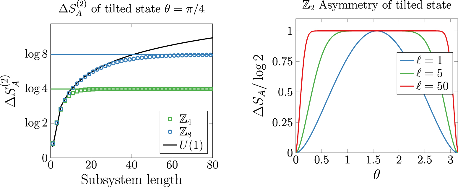
Download figure:
Standard image High-resolution image
Note that all this construction is based on the assumption that  . It is a priori possible to derive
  from other odd correlators, but we found that it is always sufficient numerically to use this expression. When
  vanishes because of oscillations after the quench, we simply used the same reasoning applied to
  and
and  to cure the divergence.