
Abstract
The bidirectional scattering-surface reflectance distribution function (BSSRDF) describes the radiance originated by the volume scattering and the surface reflectance of any position on the surface of a sample, when it is directionally irradiated at any other position. The present state of the technology for appearance rendering requires a more detailed physical description of translucent objects by traceable measurements of the BSSRDF. This work presents two primary facilities developed for traceable BSSRDF measurements by different measuring approaches. Their results on the same translucent samples have been compared and the achieved BSSRDF scale has been transferred to a commercial measuring system. This study highlights the problems of the different measuring instrument designs and provides the scientific community with more knowledge on the measurement of the BSSRDF, which will be crucial for future works on material appearance.
Export citation and abstract BibTeX RIS

Original content from this work may be used under the terms of the Creative Commons Attribution 4.0 license. Any further distribution of this work must maintain attribution to the author(s) and the title of the work, journal citation and DOI.
1. Introduction
The bidirectional scattering-surface reflectance distribution function (BSSRDF) describes the radiance originated by the volume scattering and the surface reflectance of any position on the surface of a sample, when it is directionally irradiated at any other position. Therefore, this quantity is closely related to the scattering properties below the surface and the translucent appearance of the sample [1, 2].
In recent years, the need for traceable BSSRDF measurements has increased [3]. In some domains, such as computer graphics, BSSRDF measuring systems have been developed [4–8] to meet the needs for BSSRDF data to evaluate empirical models for reproducing appearance and obtaining the optical properties of materials [9]. However, none of these systems provide traceable measurements of BSSRDF to the International System of Units (SI) and no comparison nor pilot study between different measuring systems has been performed to date.
The BSSRDF was introduced by Nicodemus et al [10] in 1977, and it is a particular example of the more general scattering function,  [11]. It is defined as follows:
where  denotes the BSSRDF,
  is the differential element of the radiance on a surface from a specific position,
  , and in a specific direction,
  , and
, and  is the differential element of the incident radiant flux on a specific position of the same surface,
  , and in a specific direction,
  . In this equation the dependence on the wavelength has been omitted for simplicity, since it is not addressed in this work.
BSSRDF is therefore an 8D function; it depends on  , defined by the spherical coordinates
  and
and  , on
, on  , defined by the coordinates
  and
and  in the sample surface reference system (SSRS), on
  , defined by the spherical coordinates
  and
and  , and on
  , defined by the coordinates
  and
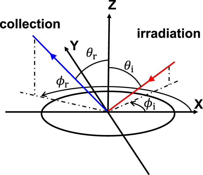
and  also in the SSRS. A scheme of the spherical coordinates is represented in figure 1.
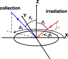
Figure 1. Scheme of the spherical coordinates that define the directions of the irradiation beam and the collection of the reflected radiance on a surface.
Download figure:
Standard image High-resolution imageDue to the many variables involved, the measurement of the BSSRDF of a sample is a complicated procedure which requires a complex measuring system. The diagram on figure 2 shows the geometrical variables involved in the measurement of the BSSRDF. In this diagram, there are no differential elements since infinitesimal quantities cannot be measured in the laboratory. Instead, the incident radiant flux that hits the surface of the sample inside the irradiated area  flows within a narrow enough' irradiation solid angle
  , and the emerging radiance from the collection area
  is measured in a 'narrow enough' collection solid angle
  . The term 'narrow enough' means, in this case, that the measurement of the BSSRDF is not affected by making the finite solid angles smaller. Furthermore, when homogeneous samples are measured, the irradiation and the collection positions on the sample surface can be reduced to the relative position of the collection with respect to the irradiation. Thus, reducing the dimensions of the function to six.

Figure 2. Diagram of the geometrical variables involved in the measurement of the BSSRDF.
Download figure:
Standard image High-resolution imageThe geometrical parameters achieved by a BSSRDF measuring system depend on the design of the system, with technical choices made to satisfy as many constraints as possible, both scientific (e.g. measurement parameters, traceability) and practical (e.g. measurement time, cost, size of the facility), with limitations caused by the complexity of the measurement. In this work, two primary facilities developed to provide traceable BSSRDF measurements are compared. One has been developed at the Instituto de Óptica 'Daza de Valdés' of the Spanish National Research Council (IO-CSIC), the designated institute in charge of the primary references for radiometry, photometry and spectrophotometry in Spain (CSIC from now on). This system is a modification of the automatic goniospectrophotometer designed and built in 2012 for absolute spectral bidirectional reflectance distribution function (BRDF) measurements [12, 13]. The other one has been developed at the Conservatoire National des Arts et Métiers (CNAM), the designated institute in charge of the primary references for radiometry, photometry and spectrophotometry in France. It shares part of the µBRDF goniospectrophotometer setup designed for BRDF measurements on tiny surfaces [14]. The main difference between these two facilities is the detection system: the goniospectrophotometer developed at CSIC uses a complementary metal–oxide–semiconductor (CMOS) sensor camera, while the detection system of the goniospectrophotometer developed at CNAM is a luminance meter. A third facility, developed at the Light & Lighting Laboratory of KU Leuven (KUL), consisting of a modified commercial near-field goniophotometer (NFG), is also involved in the study presented in this article.
The objective of this study is to demonstrate that these BSSRDF measurements have traceability to the SI and to establish a preliminary BSSRDF scale to be transferred to the measuring system developed at KUL. The work presented in this article also gives us the opportunity to better understand the impact of the parameters of our facilities on the BSSRDF measurement according to the translucency and surface properties of the measured samples.
2. Measuring systems
2.1. CSIC goniospectrophotometer
2.1.1. Measuring setup.
The BSSRDF measuring system of the CSIC was well described in [15], although some modifications have been carried out since then. The incandescent light source has been replaced by a laser driven light source (LDLS) (EQ-99X, Hamamatsu), the optical system has been optimized to obtain the maximum amount of light in the minimum feasible irradiated area, and the detection system, the charged-coupled device (CCD) camera, has been replaced by a high sensitivity CMOS camera (Orca-Flash4.0 V3, Hamamatsu). A scheme of the setup used for these measurements is shown in figure 3.
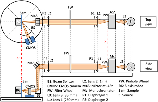
Figure 3. Diagram of the setup used in the CSIC goniospectrophotometer. P and P' represent the object and image principal planes, respectively, of the irradiation optical system.
Download figure:
Standard image High-resolution imageThe emitting plasma of the light source (S), which has a full width at half maximum (FWHM) of around 200 µm, is imaged by the lens L3 on the entrance slit of the monochromator (Mc), thus also obtaining the image at the exit slit of the Mc. Next to the Mc, a pinhole wheel (PW) has been placed. This PW contains 16 different pinhole sizes, with diameters from 20 µm to 2 mm, which allows the irradiated area on the sample surface to be modified, although in this case only one specific position of the PW has been selected for all the measurements, the smallest one (20 µm-diameter). Lenses L1 and L2 form an optical imaging system between the PW plane (P) and the sample surface plane (P') with a magnification factor  . This means that the irradiated area on the sample is approximately four times larger than the selected pinhole, without taking into account aberrations and a possible small soft focus of the image which lead to an actual irradiated area of around 140 µm in diameter. There is also a filter wheel (FW) between L1 and L2 with five different positions: clear position (no-filter), dark position (opaque filter) and three neutral density filters with nominal transmittances of 10%, 1% and 0.01%. For positioning the sample, a six-axis robot arm (R6) (Stáubli TX-40) has been used, with a mechanical holder that has a black background to minimize reflections of the light going through the samples. Lastly, for the detection, a high sensitivity CMOS camera provides a spatial resolution on the sample surface of 20 µm × 20 µm per pixel, approximately, and it is placed on a platform that can move around the sample on a cog-wheel ring.
2.1.2. Measurement model.
The BSSRDF is defined theoretically in equation (1). As mentioned in the previous section, it is not possible to measure differential quantities, so differential elements are replaced by the radiance,  , and the incident radiant flux,
  . The radiance can be expressed in terms of the reflected radiant flux,
  , as it follows [16]:
where  is the apparent area of the surface element under evaluation,
  is the actual area of this surface element,
  is the collection solid angle of the detection system and
  is the collection polar angle.
When the collection is made at  ,
,  corresponds to area of the field of view (FOV) of a pixel of the camera,
  . Nevertheless, when the collection is made at an arbitrary
  ,
,  is defined as follows:

Thus, the radiance  is expressed in terms of the geometrical parameters of the detection system:
The BSSRDF can then be expressed as a radiant flux quotient multiplied by a geometrical factor:
The radiant flux is directly related with the dark-subtracted response of a pixel of the CMOS camera, N (in units of counts), as follows:
where the factor  (with h the Planck constant and c the speed of light in vacuum) represents the inverse of the energy of a photon with wavelength λ, K is the conversion factor between photoelectrons and counts (K = 2.1 counts per photoelectron for this camera), τ is the transmittance of the camera lens,
  is the external quantum efficiency of the pixels of the CMOS sensor and
  is the exposure time. The acquisitions taken with the CMOS camera are high-dynamic-range (HDR) acquisitions. This means that the exposure time of each pixel has been adjusted to avoid low signal-to-noise ratios (SNR). Additionally, to reduce the spatial noise, a
  pixels binning was done. This means that each pixel of the binned images represents the signal of 100 pixels of the original sensor. Therefore,
  represents the area of the FOV of 100 pixels and the spatial resolution of the detection system is reduced, which is taken into account in the calculation of the BSSRDF values and its uncertainty. The obtained binned images are then projected to the SSRS through the corresponding collection polar angle,
  , in each case, as it is explained in [15].
The transmittance of the camera lens and the external quantum efficiency of the pixels may vary when measuring the incident radiant flux and the reflected radiant flux, because of the way how the light reaches the camera. In the first case, the measuring solid angle is determined by the irradiation solid angle,  , while in the second case, it is determined by the collection solid angle of the camera,
  . Thus, it is necessary to introduce a responsivity correction factor,
  , which is defined as [15]:
where indexes 'r' and 'i' refer to reflected and incident radiant flux measurements, respectively. Furthermore, for the measurement of the incident radiant flux, the neutral density filter of the FW with a nominal transmittance of 0.01% had to be used to avoid the saturation of the pixels of the CMOS sensor. Therefore, the measurement equation of the BSSRDF in the goniospectrophotometer at CSIC becomes:
where  represents the BSSRDF value of the binned pixel 'k',
  is the transmittance of the neutral density filter used for the incident radiant flux acquisition,
  and
and  are the response in counts of the binned pixel 'k' for the reflected radiant flux acquisition and the incident radiant flux acquisition, respectively, and
  and
and  are the exposure times used by the binned pixel 'k' in the reflected radiant flux acquisition and in the incident radiant flux acquisition, respectively.
  is a correction factor accounting for the non-linearity of the response of the pixel 'k'.
The square of the relative standard uncertainty of the BSSRDF can be expressed as the quadrature sum of the relative standard uncertainties of all variables involved in equation (8):
This equation is fulfilled since the errors on the values of the variables involved in the measurement equation are not correlated, except for the term of the sum of the response of the binned pixels in the incident radiant flux acquisition, which is fully correlated. Nevertheless, as the response of the reflected radiant flux acquisition is divided by the incidence radiant flux acquisition with the same camera, this correlation is canceled. On the other hand, it is true that the errors of the BSSRDF values at different geometries are correlated, which should be taken into account when integrating these values to obtain another magnitude from the BSSRDF, but it does not affect the uncertainty of each BSSRDF value to be compared. The estimation of the uncertainty of integrated magnitudes is out of the scope of our current research, but it should be address in the future, likely through the Monte Carlo method [17] due to the complexity of the measurement.
Strictly speaking, the uncertainties introduced by the angular and spatial resolutions of the measuring system should also be accounted in equation (9). Nevertheless, they depend on the specific characteristics of the sample being measured, making necessary to have a prior characterization of the BSSRDF of the sample. The samples that have been measured in this work present a very smooth angular distribution far from the specular direction and a smooth spatial distribution outside the irradiated area, and both conditions are fulfilled for the compared BSSRDF values. Furthermore, the robot arm and the detection platform are very precise, so the error in the angle is supposed to be very small, as the error in the  position on the sample surface, since the detection system has a very high spatial resolution. These effects can be neglected because their contribution is supposed to be much smaller than other main uncertainty sources present in the current measurements of the BSSRDF as the noise due to the response of the pixels.
2.1.3. Uncertainty sources
2.1.3.1. Area of the detection FOV on the sample plane,  .
.

To measure  a calibrated 10 mm stage micrometer with 50 µm divisions was used. It was placed on the sample plane and it was irradiated with a broadband uniform beam. Then, an horizontal and a vertical image of the micrometer were taken with the CMOS camera in transmittance, using the same acquisition configuration as in the measurements. The horizontal and vertical dimensions of the pixels in mm on the sample surface were obtained from the number of pixels between the first and the last division of the micrometer, resulting the multiplication of both dimensions in
  . Thus, the relative standard uncertainty of
  is determined by the standard deviation of the number of pixels of four repetitions and the uncertainty on the calibration of the stage micrometer, and it was estimated at 0.1% by applying the uncertainty propagation law.
2.1.3.2. Dark-subtracted binned pixel response, Nk .
The analysis of the uncertainty due to the response of the pixels of the CMOS camera is essentially the same as explained in [15], but now the noise parameters of the camera are different, since the CMOS camera has replaced the previous CCD camera. The readout noise,  , of the new detection system was estimated at 0.86 e− rms, the conversion factor, K, at 2.1 counts per e−, and the mean thermal electrons rate of the CMOS sensor,
  , at 0.011 e− s−1 per pixel. The method used for the estimation of the correction factor is described in the literature [18]. The standard uncertainty of the dark-subtracted response of the pixel 'j',
  , becomes:

where  is the rate of the electrons generated per pixel by the stray light in the laboratory in the moment of the measurement and the factor 2 comes from the two acquisitions needed for subtracting the dark signal.
The dark-subtracted binned pixel response is the result of summing the dark-subtracted response of 100 pixels, thus its uncertainty is the square root of the quadrature sum of the uncertainty of each single pixel. The relative standard uncertainty of the dark-subtracted binned pixel response is therefore:
where  is calculated from equation (10) and the additions include the 100 pixels that are being accounted for the binned pixel 'k'. Since
  and
and  are almost constant for a given bin 'k', the impact of the noise in the relative uncertainty is reduced approximately by a factor of 10.
2.1.3.3. Transmittance of the neutral density filter, .

The transmittance of neutral density filters was measured with a calibrated spectrophotometer in the past (see [12]). A relative standard uncertainty of 0.48% was obtained for the filter with a nominal transmittance of 0.01%, the one used for measuring the incident radiant flux.
2.1.3.4. Collection solid angle, .

The calculation of the collection solid angle and its uncertainty analysis was carried out following the same procedure as explained in [15] but now with the CMOS camera. In this case, the angular steps were reduced from 1° to 0.5°, and the resulting relative standard uncertainty became 0.23%.
2.1.3.5. Exposure time, .

The uncertainty of the exposure time used by each pixel of the CMOS sensor is very small compared to the minimum integration time used in the acquisitions. So, the relative standard uncertainty of the exposure time ratio can be considered negligible.
2.1.3.6. Responsivity correction factor, .

The responsivity correction factor is obtained from the measurement data of the collection solid angle, and its calculation is also explained in [15]. Its relative standard uncertainty for the CMOS camera is 0.19%.
2.1.3.7. Non-linearity correction factor, .

The non-linearity of the CMOS sensor was corrected using the methods described in [19]. Nevertheless, the applied correction factors have a relative standard uncertainty estimated at 0.6%.
2.2. CNAM goniospectrophotometer
2.2.1. Measuring setup.
The goniospectrophotometer setup for BSSRDF measurements at CNAM, shown in figure 4, has been designed to perform an absolute measurement of BSSRDF and is described in [20]. The sample, held on a robot arm, is illuminated by a narrow and directional light beam. The reflected radiance is measured over a small area in the collection direction using a luminance meter as a detection system. Contrary to a camera-based detection, the luminance meter provides a single value of luminance for the area within the FOV. It is therefore combined with a spatial scanning system (i.e. translation stages) to measure luminance at any location on the sample.
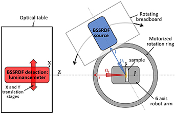
Figure 4. The CNAM goniospectrophotometer for BSSRDF measurement (top view).
Download figure:
Standard image High-resolution imageThe source of this setup has been designed to illuminate the sample with a very bright and thin beam. It comprises an LDLS (EQ-99X, Hamamatsu) and an optical system optimized to obtain a light spot with a diameter of about 50 µm on the sample. This source is shared with CNAM's 'µBRDF' setup and is described in detail in [14]. The source is located on a breadboard and can be rotated around the sample in the horizontal plane using the rotation ring. The incident flux on the sample is measured by placing the source directly in front of the detection system. The source aperture is adjusted to 1.5° to ensure no vignetting on the detection system for the source direct measurement while maximizing optical power. The detection system is a luminance meter (Pritchard) equipped with a photomultiplier tube. This allows to measure luminance as low as  cd m−2. The diameter of the detection FOV on the sample plane, which limits the spatial resolution of the measurements, is about 1 mm. The sample is held at the center of the goniospectrophotometer by a six-axis robot arm (RV-12S, Mitsubishi). For BSSRDF measurements, the robot has its wrist oriented upward and the sample is held vertically by a clamp. In this way, light can be freely transmitted through the sample with no risk of back reflection. Using the robot rotations and the rotation ring, sample and source are oriented to meet the chosen geometry of measurement for the incident beam and collection directions (
 and
and  ). The location of the incident beam (
 ) can be controlled by using the translation tools of the robot arm.
The X and Y translations to be applied to the detection system for observing the reflected radiance from the position  on the sample surface are determined by the geometry of measurement. The location of the collection point in the coordinate system of the detection can be obtained by applying to the vector (
 ,
,  , 0) three consecutive rotations of angle β around the x-axis, α around the y-axis and γ around the z-axis, with (
 ) angles that describe the orientation of the sample and that are linked to the angular geometry of measurement (
 ,
,  ,
,  ,
,  ) using formulas given in [21]. In the study presented in this paper, only in-plane measurements were performed, which simplifies the calculation of the detection position:


2.2.2. Measurement model.
The BSSRDF,  , is defined as the ratio of the reflected radiance
  to the incident radiant flux
  . The incident radiant flux is measured by placing the source directly in front of the detection system. In this configuration, the detection system measures the luminance
  and the associated dark signal
  . The incident radiance flux is then calculated using the following equation:

with  being the area of the detection FOV on the sample plane and
  the collection solid angle.
The reflected radiance is measured after placing the source, the detection system and the sample in the chosen geometry of measurement. The luminance meter directly measures the luminance  and the associated dark signal
  . Finally, the measurement equation for BSSRDF is:
The relative standard uncertainty of the BSSRDF,  , can be related to the uncertainties on each variable of equation (15) as follows:
In this first study, the uncertainties induced by angular and spatial positioning errors are only partially accounted for from the repeatability measurement. As light becomes increasingly diffuse with subsurface scattering, negligible uncertainties are expected to be induced by errors on the angular positioning of the sample. Errors on the spatial  position of the sample have a higher impact, especially close to the center, and will be thoroughly evaluated in future works.
2.2.3. Uncertainty sources
2.2.3.1. Luminance meter response, L.
The luminance  was independently measured three times for each sample. The uncertainty on
  is given by the standard deviation on the measurement divided by
  . The value of the uncertainty
  is strongly impacted by sensor noise and gets high when the signal is very low: it is inferior to 5% (and as low as 1%) when the measured luminance is superior to 0.2 cd
  , and as high as 50% when the measured luminance is lower than 0.001 cd
  .
.
The uncertainty on  has been evaluated at 2.4%. This uncertainty accounts for the reproducibility of the measurement, evaluated by asking the operator to realign the instrument in front of the source for 10 independent measurements. This uncertainty also accounts for the instrument resolution and the non-linearity of the luminance meter, which is used in a high-dynamic mode for measurements on the sample, but in a low-dynamic mode for the direct measurement of the source.
The uncertainty on  and
and  has also been statistically evaluated at 1.4%. This value accounts for stray light, sensor noise and instrument resolution.
2.2.3.2. Area of the detection FOV on the sample plane, .

The area  was measured by taking a photograph of a ruler placed on the sample plane with the viewfinder of the luminance meter. The relative standard uncertainty for this measurement is 6.7%, limited by the poor accuracy that can be achieved in measuring the FOV diameter. When the measured luminance signal is not too noisy, this component constitutes the largest contribution to the total uncertainty.
2.2.3.3. Collection solid angle, .

The luminance meter comprises a lens that creates some vignetting and yields a non-uniform luminance measurement over the collection solid angle. Consequently, the solid angle can be expressed as:
where  is the equivalent aperture area that accounts for the luminance distribution within the solid angle, and d is the distance between the sample and the detection's entrance aperture. The equivalent aperture area is
  (43.2 mm for the equivalent diameter) and the sample to aperture distance is 1.931 m.
The luminance distribution over the collection solid angle can be estimated by placing an iris diaphragm just in front of the lens (which corresponds to the position of the detection's entrance aperture), and by measuring the luminance of a uniformly illuminated sample for various apertures of the iris diaphragm. To compute the equivalent aperture area  , two luminance measurements were performed on an uniformly illuminated Spectralon sample. First, the iris diaphragm diameter was chosen small enough (24 mm) to ensure that the light going through the luminance meter lens was not vignetted and the luminance
  was measured with a diaphragm of area
  . Then, the iris diaphragm was removed, and the luminance
  was measured. Assuming that the luminance distribution is uniform at the center of the FOV of the luminance meter, the equivalent aperture area is given by:
The relative uncertainty on the equivalent aperture area (2.6%) and on the sample to aperture distance (0.5%) yields the relative uncertainty on the collection solid angle, which is 2.8%.
2.3. KUL goniophotometer
2.3.1. Measuring setup.
The BSSRDF measurement facility at KUL (Light & Lighting Laboratory) is a modified commercial NFG, type Rigo 801-300 (TechnoTeam GmbH). This is the system to which the BSSRDF scale was transferred. Typically, an NFG is used to measure ray files and radiation patterns from light sources. However, as the measurement device is equipped with a calibrated imaging luminance measurement device (ILMD), it can be modified to also measure BSSRDF. The modifications to the NFG include a customized laser illumination setup and sample holder.
The illumination part, shown in figure 5, consists of a laser diode (532 nm, type CPS532 - 4.5 mW) followed by an aperture of 1 mm in diameter. This aperture is imaged toward the center of the NFG using a lens with a focal length of 33 cm. The resulting illumination spot at the center of the NFG has a diameter of 2.6 mm. In order to minimize laser speckle, a rotating front surface diffuser, which has a bidirectional transmittance distribution function with FWHM of 8°, is positioned between the laser and the aperture. The collimated laser beam is enclosed by a hollow metal tube onto which the sample holder at the center of the NFG is attached.
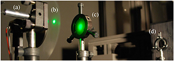
Figure 5. Illumination system attached to NFG consisting of a 4.5 mW laser diode (a), a rotating diffuser (b), a 1 mm diameter aperture (c) and a lens with a focal length of 33 cm (d).
Download figure:
Standard image High-resolution imageDuring normal NFG operation, this hollow metal tube is used to provide electrical connections to the light source to be measured. During BSSRDF measurements, a sample holder is positioned at the center of the NFG, as is shown in figure 6. The sample holder, which was custom designed and 3D printed, allows for various angles of incidence within a single plane (i.e. only the polar incident angle can be manually altered, while the azimuthal incident direction is fixed).
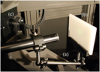
Figure 6. Sample holder (a) mounted within the NFG holding a polycarbonate translucent sample (b), and the ILMD system (c).
Download figure:
Standard image High-resolution imageAlignment of the sample is done using the same alignment procedure as when measuring light sources with the NFG. During this procedure a live view of the ILMD is shown with an overlay of the internal coordinate system of the NFG. This allows the front surface of the sample to be positioned exactly at the center. Next, the incident angle is set manually by rotating the sample holder, reading the spatial offsets of the edges of the sample from the ILMD live view, and calculating the corresponding angle of incidence.
Once the sample is aligned, the rotating arm onto which the ILMD is mounted is rotated to capture multiple HDR luminance images from different viewing directions. The FOV of the ILMD can be adjusted by changing the ILMDs lens. For the BSSRDF measurements in this article, a lens with an FOV of 80 mm was chosen.
2.3.2. Measurement model.
Although this is not a primary facility developed for traceable BSSRDF measurements, it provides BSSRDF measurements with SI units through the comparison with a Spectralon calibration tile whose spectral radiance factor [22] for a geometry of 0°:45°,  , is known. The BSSRDF measurement equation for this measuring setup is the following:
where  and
and  denote the luminance of the pixel 'k' of the HDR luminance image of the measured sample and the calibration tile, respectively,
  is the collection polar angle and
  the area of the FOV of a pixel of the ILMD.
2.4. Comparison of geometrical parameters
The three measuring systems described above show different technical choices, which yield slightly different geometrical parameters for the measurement of the BSSRDF (namely, the size of the irradiation beam, the collection area and the irradiation and collection solid angles). An overview of the geometrical parameters of each measurement facility is shown in table 1.
Table 1. Geometrical measurement parameters of each BSSRDF measuring system.
| Partner |
A
 /mm2 /mm2
|
A
 /mm2 /mm2
|
 /sr /sr |
 /sr /sr |
|---|---|---|---|---|
| CSIC |

|

|

|

|
| CNAM |

| 1.1 |

|

|
| KUL | 5.3 |

|

|

|
As mentioned earlier, the BSSRDF is theoretically defined for infinitesimal quantities, but realized in practice by measuring light from areas of finite size and within finite solid angles (see figure 2). The BSSRDF measured on a sample should describe the intrinsic properties of the sample, i.e. without any influence from the geometrical parameters of the measuring system. Nevertheless, this influence is sample-dependent, since it depends on the shape of the BSSRDF to be measured, and therefore depends on the scattering properties of the material as well as the surface properties of the sample. A sample with a smooth BSSRDF distribution, both angularly and spatially, will be less influenced by the geometric parameters compared to a sample with a highly variable BSSRDF distribution. For instance, it has been shown that measurement parameters are critical for collection positions that are inside or at the border of the irradiated area [23], since in these positions both surface-reflected light and volume-scattered light are being accounted in the detection and the BSSRDF actually depends on the irradiated area. Therefore, in these positions the measured BSSRDF value may significantly vary between the three measurement facilities presented in this work.
3. Comparison between CSIC and CNAM measurements
The measurand of this comparison is the BSSRDF of three translucent samples with different levels of translucency (samples A, B and C, from more opaque to more transparent, see figure 7) at three different in-plane measurement geometries and at different positions on the sample surface from  mm to x = 6 mm with y = 0 mm with respect to the center of the irradiated area (see figure 2). The three different measurement geometries are specified in table 2 by their corresponding spherical coordinates (see figure 1).

Figure 7. Translucent samples manufactured by Covestro Deutschland AG for BSSRDF comparison.
Download figure:
Standard image High-resolution imageTable 2. Measurement geometries of the comparison.
| Geometry |
 /° /° |
 /° /° |
 /° /° |
 /° /° |
|---|---|---|---|---|
| 0°:45° | 0 | 45 | 0 | 180 |
| 45°:0° | 45 | 0 | 0 | 180 |
| 60°:15° | 60 | 15 | 0 | 180 |
The more challenging geometries in the measurement are those with larger incidence and collection angles, as in the case of BRDF measurements. Technically, the realization of out-of-plane geometries is complex, although it recently has been proved that it is well solved for traceable BRDF measurements [24]. These issues will be addressed in future works once the traceability of the BSSRDF measurement has been consolidated at these more simple selected geometries.
The BSSRDF values reported by CNAM do not correspond to an spectral illumination, as is the case of CSIC at 550 nm, but to an effective spectral value at 555 nm, obtained by weighting with the spectral distribution of the luminous efficiency curve [25]. However, since the samples present a white or gray color and are illuminated with a rather neutral spectral distribution in the case of CNAM, it has been assumed that the difference between the values due to the spectrum is negligible with respect to the sources of measurement uncertainty considered in this work. Of course, strictly speaking, these differences have to be taken into account in the uncertainty budget of the comparison itself, which has not been considered in this work, together with other sources of uncertainty such as temperature.
The samples were custom manufactured by the company Covestro Deutschland AG. They consist of a polymer matrix (polycarbonate) with n = 1.585 at λ = 589.3 nm in which scattering particles with controlled mean diameter sizes have been added at controlled mass concentrations. The specifications of the added scattering particles for each sample are given in table 3. All the samples have the same dimensions: 150 mm × 105 mm × 6.4 mm. The samples are very flat in all cases, leading to limited surface scattering at non-specular directions (the maximum difference in height on their surfaces is less than 1 µm). Thus, the translucent properties of these samples should be dominated by the volume scattering inside the sample matrix. However, in the overlap region between the illuminated and collected area, even a limited amount of surface scattering can have a large impact on the BSSRDF.
Table 3. Specifications of the samples given by the manufacturer.
| Samples | A | B | C |
|---|---|---|---|
| Mean diameter of scattering particles/µm | 0.3 | 2.2 | 8–10 |
| % Mass of scattering particles | 3.0 | 0.65 | 3.0 |
Refractive index at  589.3 nm 589.3 nm | — | 1.420 | 1.535 |
The BSSRDF measurements from CSIC and CNAM are shown in figure 8 [26], where each row of plots corresponds to each sample and the columns of plots correspond to the measurement geometries. The y-axis of the plots is in logarithmic scale and represents the BSSRDF value, while the x-axis represents the x-position of the collection area with respect to the center of the irradiated area (see figure 2). Its absolute value thus corresponds to the distance between collection and irradiation positions, since the y-coordinate equals zero (y = 0) in the presented plots. Analogously, the corresponding relative expanded uncertainties,  , are represented in figure 9. Since the detection system used at CNAM uses a spatial scanning system, its measured relative positions on the sample surface do not precisely agree with the relative positions corresponding to the binned pixels of the images taken with the detection system used at CSIC. Therefore, as the detection system used at CSIC spatially provides more data, the BSSRDF values and uncertainties reported by CSIC have been spatially interpolated to match the positions measured at CNAM. CNAM was not able to measure the most transparent sample (sample C) due to the very low SNR, so no results are shown for this sample from CNAM measurements. Additionally, the uncertainty budget of CSIC and CNAM facilities for three specific positions (p1, p2 and p3) located at x = 1.1 mm,
  mm and
  mm, respectively, of the surface of sample B measured at 45°:0° geometry is shown in table A1 and table A2, respectively, of the
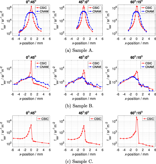
Figure 8. Measured BSSRDF values of the samples (a) A, (b) B and (c) C at CSIC (red line with ' ' markers) and CNAM (blue line with '
 ' markers). See online version for colored plots.
Download figure:
Standard image High-resolution image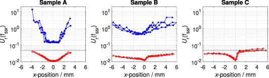
Figure 9. Relative expanded uncertainty (k = 2) of the measurement of the BSSRDF for each facility (red lines with open markers for CSIC and blue lines with full markers for CNAM) each sample and each measurement geometry ( /
/ for 0°:45°,
  /
/ for 45°:0° and
  /
/ for 60°:15°). The line '- - - -' indicates a relative expanded uncertainty of 5%. See online version for colored plots.
Download figure:
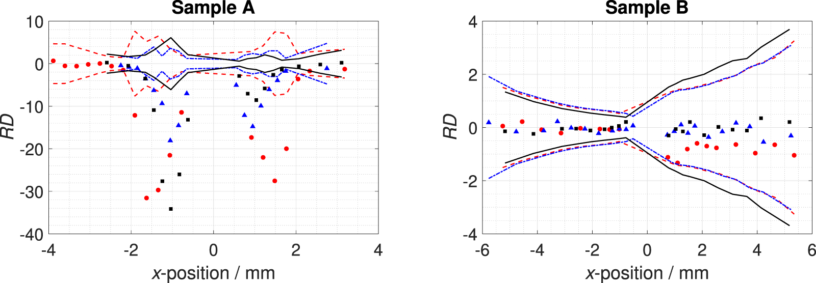
Standard image High-resolution imageAs seen in figure 8(a), the comparison between CSIC and CNAM is not good for sample A. For this sample, the BSSRDF decreases really fast outside the irradiated area. As the detection system used by CNAM averages all the reflected radiant flux inside a collection disk of 1 mm diameter approximately, the values measured by CNAM do not represent the rapid spatial variation of the BSSRDF. This explains why CNAM's results differ significantly from the measured values at CSIC for this sample. The same effect can be observed in the comparison for sample B (figure 8(b)). However, in this case, the effect of the collection disk is not appreciable outside the irradiated area because the volume-scattered light is more spatially distributed, and the BSSRDF distribution is thus much smoother. The measurements agree well outside the irradiated area, where all the light comes from volume scattering events inside the sample. This good agreement is quantified in figure 10 by the relative difference, RD, between the BSSRDF values measured at CSIC and at CNAM, calculated as:

Figure 10. Relative difference of the BSSRDF values measured at CSIC and at CNAM, normalized to the values from CSIC, for samples A (left) and B (right) and for each measurement geometry (red  for 0°:45°, blue
  for 45°:0° and black
  for 60°:15°). The lines represent the combined expanded uncertainty bounds of the measures for each geometry ('- - - -' for 0°:45°, '—.—' for 45°:0° and '—' for 60°:15°). Colored plots are available in the online version.
Download figure:
Standard image High-resolution image
where  and
and  represent the BSSRDF value measured at CSIC and CNAM, respectively.
Figure 10 shows the RD between CSIC and CNAM measurements for samples A and B at each measurement geometry. For the sake of clarity, the values at the positions in which the reflected radiant flux measured by CNAM may account surface-reflected light have been omitted. For sample A, the RD is high in absolute value and it is outside the combined expanded uncertainty bounds. This means that the measurements from both systems are not compatible for this sample, but this incompatibility has been explained in the previous paragraph. For sample B, however, the values of the RD are inside the combined expanded uncertainty bounds; therefore, the measurements from both systems are compatible. Nevertheless, compatibility can be assessed more explicitly by calculating the compatibility coefficient, according to the following equation:
where  represents the BSSRDF value measured at CSIC (or CNAM) and
  is the corresponding expanded uncertainty (k = 2). Typically, two measurements are regarded as compatible when the absolute value of C is lower than 1. The results are represented in figure 11, where the values at the positions with surface-reflected light contribution have been omitted too.
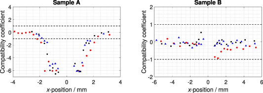
Figure 11. Compatibility coefficient between the BSSRDF measurements of CSIC and CNAM for samples A (left) and B (right) and for each measurement geometry (red  for 0°:45°, blue
  for 45°:0° and black
  for 60°:15°). The lines '- - - -' represent the bounds within two measurements can be considered compatible. Colored plots are available in the online version.
Download figure:
Standard image High-resolution imageThe low compatibility coefficient values for sample B are due to the high noise of the detection in CNAM measurements. In sample A, measurements at positions close to the irradiated area present incompatibility for all geometries. This incompatibility is explained by the effect of the large collection area of the CNAM facility.
4. BSSRDF scale transfer to KUL
One important objective of this research was to study the transfer of the BSSRDF scale from a primary facility to a non-primary facility, which needs an external calibration sample to provide traceability to its BSSRDF measurements. The sample B is the most adequate as transfer standard, because the BSSRDF values can be assessed for more limited instruments, with lower resolution or sensitivities, as demonstrated in the results shown in figure 8(b). The other samples, however, could be included in a set of transfer standards which would allow the instrument to be calibrated for three types of samples with very different scattering behavior. The transfer of the BSSRDF scale is done by comparing the BSSRDF measurements of the transfer standard by the system to be calibrated with the better estimations of the BSSRDF, previously determined for a number of measuring conditions (geometries, positions and wavelengths, in this case) by SI-traceable methods and primary facilities, as described before. This comparison allows the calibration factor of the instrument to be calculated, and systematic errors to be identified.
The transfer of the BSSRDF scale was studied for the KUL measuring system, using the sample B as transfer standard. Given the high relative uncertainty obtained at CNAM, it was decided to consider the measurements at CSIC as the better estimation of the BSSRDF. The illumination wavelength used at KUL is 532 nm, slightly different to the one used at CSIC. The results obtained at KUL, in comparison with those from CSIC, are shown in figure 12 [26]. The correction factor,  , for this facility was obtained by dividing the BSSRDF values from CSIC (better estimation) by the measurements at KUL, and the results of this calculation are shown in figure 13.
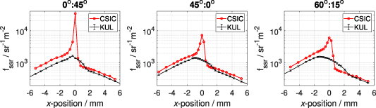
Figure 12. Measured BSSRDF values of the sample B at CSIC (red line with ' ' markers) and KUL (black line with error bars). The error bars of the KUL values represent the expanded uncertainty (k = 2) of their measurements. See online version for colored plots.
Download figure:
Standard image High-resolution image
Figure 13. Ratio between BSSRDF measurements at CSIC and BSSRDF measurements at KUL of sample B for each measurement geometry (red  for 0°:45°, blue
  for 45°:0° and black
  for 60°:15°). The error bars represent the expanded uncertainty (k = 2) of the ratio. Colored plot available in the online version.
Download figure:
Standard image High-resolution imageFigure 12 shows a good agreement between both measurements regarding the shape of the BSSRDF profile in the positions that are outside the KUL irradiated area, although there is a small systematic difference in the values higher than the expanded uncertainty of KUL measurements. In figure 13, the values that correspond to positions inside the KUL irradiated area have been omitted. It is seen that this ratio is approximately constant regarding the distance to the irradiated area, but it seems to depend on the measurement geometry, since it is higher for the 0°:45° geometry than for the other two geometries, 45°:0° and 60°:15°, where the collection direction is normal or almost normal to the sample surface, respectively. This could be related to a bad compensation of the collection angle. However, this behavior does not persist in the positions that are on the incidence semi-plane ( ). There, the ratio is lower and does not seem to depend on the measurement geometry. This could be conditioned by some misalignment of the center of the irradiated area at KUL measuring system, since it is much bigger than the irradiated area of CSIC measuring system and its center is located with lower accuracy. Also, other uncertainty sources not considered in this work, such as the illumination wavelength, can be affecting in a lesser extent.
5. Discussion
The obtained results of this study show that there are two principal issues that must be taken into account when measuring the BSSRDF and, although their effect on the results may seem very similar, their origin is completely different. These are the lack of spatial resolution in the detection and the use of a large irradiated area on the sample surface.
On one hand, in the comparison between CSIC and CNAM measurements, the results presented in figure 8 show that a low spatial resolution of the detection system can lead to a loss of information of the spatial distribution of the BSSRDF. For some samples this can occur only in certain regions of the surface where the BSSRDF present a rapid spatial variation, e.g. sample B (see figure 8(b)), but for others it can prevent the correct characterization of the BSSRDF of the sample at all, e.g. sample A (see figure 8(a)). As a demonstration, the BSSRDF values measured at CSIC have been convoluted within an area as large as the collection area of the system developed at CNAM. This procedure clearly reduces the differences between CSIC and CNAM measurements on sample A, as shown in figure 14. These large observed differences in the comparison between CSIC and CNAM measurements are thus mainly due to the larger measurement area of the system developed at CNAM.
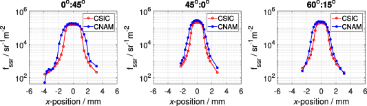
Figure 14. Convoluted BSSRDF values from CSIC (red lines with ' ' markers) of sample A compared with the BSSRDF values measured at CNAM (blue lines with '
 ' markers). See online version for colored plots.
Download figure:
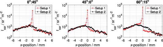
Standard image High-resolution imageOn the other hand, in figure 12 the main difference in the values seems to be due to the KUL irradiated area, which is more than ten times larger than the irradiated area used at CSIC. In this case, the main difference is only at the positions that are inside the irradiated area of the KUL setup. As a demonstration of this effect, a Monte-Carlo ray-tracing simulation (with 25 million rays) is performed for a translucent sample with similar volume and surface scattering properties as sample B (see modeling parameters in table 4). The resulting BSSRDF is simulated for two setups with a different irradiated area: in one case equal to the irradiated area for the CSIC setup and in the other case equal to the irradiated area for the KUL setup. The results are shown in figure 15, and it is observed a similar deviation of the results as in the experimental comparison of the CSIC and KUL setup for sample B.
Figure 15. Simulated BSSRDF values for sample B, for the case with an irradiated area equal to the CSIC (setup 1, red lines with ' ' markers) and KUL setup (setup 2, black lines with '
 ' markers). See online version for colored plots.
Download figure:
Standard image High-resolution image
Table 4. Modeling parameters of the simulated BSSRDF values of figure 15.
| Mie scattering assumption | ||
| Volume scattering | Particle size: 1100 nm | |
| Particle refractive index: 1.42 | ||
| Matrix refractive index: 1.589 | ||
| % Mass of scattering particles: 0.65% | ||
| Harvey–Shack scattering assumption | ||
| Surface scattering | Intercept (b0): 706 
| |
| Shoulder angle: 2° | ||
| Slope: -3 | ||
| Surface roughness RMS: 100 nm | ||
| Setup 1 | Setup 2 | |
| Measurement setup configuration |

|

|

| ||
 sr sr | ||
 sr sr | ||
As mentioned before, the dependence of the BSSRDF on the irradiated area at those positions was already shown in the literature [23], and it is due to the co-existence of two different phenomenon's: surface scattering and volume scattering. While the radiance from the second one is proportional to the total incident radiant flux on the material and is characterized by the BSSRDF, the radiance from the first one is proportional to the irradiance on the surface and, therefore, is not well characterized by the BSSRDF. Thus, it is better to use a smaller area to irradiate the sample (always keeping the SNR acceptable) to evaluate the correct BSSRDF in a wider range of the sample surface.
This study also allowed us to compare several instrument designs and observe the impact of the geometrical measurement parameters on the BSSRDF. The results show that a camera-based system like the one developed at CSIC yields better results on a wider range of translucent samples thanks to its higher spatial resolution and lower noise. This kind of system should be more adequate for industrial applications, as it can provide BSSRDF measurements faster than using a detector without spatial resolution. Furthermore, the measurement results obtained with the facility developed at CNAM illustrates that using a luminance meter for detection is not adapted to almost transparent samples or to samples with high reflectance due to its low sensitivity and the difficulties to provide a comparatively high spatial resolution by scanning, since its FOV is much more limited that the FOV of the pixels of typical cameras. Nevertheless, for targeted measurements, this kind of design might provide a conventional route for traceability. Also, systems based on commercial NFGs, as the one used at KUL, seem to be a good simple solution to perform BSSRDF measurements.
6. Conclusions
The BSSRDF scale realized by two different primary measurement facilities (developed at CSIC and CNAM) has been compared through the measurement of three samples with different levels of translucency specifically produced for this study. The measurements on sample A (the most opaque) and sample C (the most transparent) allowed the complexity of the measurement to be understood for such extreme cases. Besides, the consequence of using a poor spatial resolution on the BSSRDF measurements has been demonstrated. For a more intermediate case, as the translucent sample B, the BSSRDF measurements showed a good agreement between the two facilities, being possible to establish a primary BSSRDF measurement scale.
In addition, the transfer of the achieved BSSRDF measurement scale has been studied for the measuring system at KUL. The relative values of the BSSRDF measurements at KUL agree well with the previously obtained values from the comparison between CSIC and CNAM, and a calibration factor for this facility was obtained. We observed some dependence of this calibration factor on the geometry and on the position on the sample, which might be a consequence of the different realization of the bidirectional geometry and the size of the irradiated area. These effects should be carefully studied in future works. From these results, also the impact of the irradiation area on the BSSRDF measurements was demonstrated.
In summary, the present work shows the high complexity of the BSSRDF measurements and provides some important guidelines for future developments of BSSRDF measuring systems
Acknowledgment
This work has been done in the frame of the project 18SIB03 BxDiff, that has received funding from the EMPIR programme co-financed by the Participating States and from the European Union's Horizon 2020 research and innovation programme. P Santafé-Gabarda, A Ferrero and J Campos would also like to acknowledge Project PGC2018-096470-B-I00 BISCAT (MCIU/AEI/FEDER,UE) and Comunidad de Madrid, Grant Number S2018/NMT-4326-SINFOTON2-C. We are grateful to Covestro Deutschland AG for providing us with translucent samples.
Data availability statement
The data that support the findings of this study are openly available at the following URL/DOI: https://zenodo.org/communities/bxdiff/.
Appendix:
Table A1. Uncertainty budget of CSIC goniospectrophotometer for three specific positions (p1, p2 and p3) located at x = 1.1 mm,  mm and
  mm, respectively, of the surface of sample B measured at 45°:0° geometry.
| Relative uncertainty (k = 1) | ||||
|---|---|---|---|---|
| Source of uncertainty | Variable | p1 | p2 | p3 |
| Dark-subtracted pixel response |

| 0.88% | 0.54% | 0.63% |

| 0.033% | 0.033% | 0.033% | |
| Area of the detection FOV |

| 0.10% | 0.10% | 0.10% |
| Transmittance of the ND filter |

| 0.48% | 0.48% | 0.48% |
| Collection solid angle |

| 0.23% | 0.23% | 0.23% |
| Responsivity correction factor |

| 0.19% | 0.19% | 0.19% |
| Non-linearity correction factor |

| 0.60% | 0.60% | 0.60% |
Table A2. Uncertainty budget of CNAM goniospectrophotometer for three specific positions (p1, p2 and p3) located at x = 1.1 mm,  mm and
  mm, respectively, of the surface of sample B measured at 45°:0° geometry.
| Relative uncertainty (k = 1) | ||||
|---|---|---|---|---|
| Source of uncertainty | Variable | p1 | p2 | p3 |
| Luminance meter response |

| 25% | 20% | 29% |

| 2.4% | 2.4% | 2.4% | |

| 1.4% | 1.4% | 1.4% | |

| 1.4% | 1.4% | 1.4% | |
| Area of the detection FOV |

| 6.7% | 6.7% | 6.7% |
| Collection solid angle |

| 2.8% | 2.8% | 2.8% |