


Abstract
The discovery of two thin rings around the ∼ 250 km sized Centaur Chariklo was the first of its kind, and their formation and evolutionary mechanisms are not well understood. Here, we explore a single shepherd satellite as a mechanism to confine Chariklo's rings. We also investigate the impact of such a perturber on reaccretion, which is a likely process for material located outside the Roche limit. We have modified N-body code that was developed for Saturn's rings to model the Chariklo system. Exploration of a reasonable parameter space indicates that rings like those observed could be stable as the result of a single satellite with a mass of a few ×1013 kg that is in orbital resonance with the rings. There is a roughly linear relationship between the model optical depth and the mass of the satellite required to confine a ring. Ring particles do not accrete into moonlets during hard-sphere simulations. However, a reasonable fraction of the ring material forms into moonlets after a few tens of orbits for soft-sphere collisions. The ring-particle properties are thus key parameters in terms of moonlet accretion or destruction in this system.
Export citation and abstract BibTeX RIS

Original content from this work may be used under the terms of the Creative Commons Attribution 4.0 licence. Any further distribution of this work must maintain attribution to the author(s) and the title of the work, journal citation and DOI.
1. Introduction
In 2013, a multi-chord stellar occultation by (10199) Chariklo revealed a system of two thin rings, referred to as C1R and C2R (Braga-Ribas et al. 2014). Chariklo is the largest known Centaur. It orbits from ∼13 to 18.5 au, with an eccentricity of 0.17, inclination of 23°, and spin rate of 7.004 ± 0.036 hr (Fornasier et al. 2014). From infrared data, Chariklo's diameter was estimated to be 248 ± 18 km (Fornasier et al. 2013). The newly discovered rings were located approximately 391 and 405 km from the center of the nucleus, with widths of roughly 7 and 3 km and normal optical depths of 0.31–0.46 and 0.04–0.12, respectively (Braga-Ribas et al. 2014).
Analyses of additional stellar occultations by Chariklo from 2014 to 2020 (i) confirmed the circular ring solution and pole position from 2013 to within the error bars, (ii) determined that C1R blocks roughly ten times more light than C2R (with equivalent widths of roughly 2 km and 0.02 km, respectively), (iii) estimated the eccentricity of C1R to be 0.005–0.022, (iv) found that C1R and C2R vary azimuthally in width by up to 4.3 and 1 km, respectively, (v) revealed a W-shaped structure in C1R, and (vi) noted that the rings are located close to the 3:1 resonance between Chariklo's rotation and the ring orbit, which is at 408 ± 20 km (Bérard et al. 2015; Leiva et al. 2017; Morgado et al. 2021). The most recent analysis found Chariklo to be a triaxial ellipsoid with semi-axes of  ,
,  , and
, and  km, and the rings were measured at radii of 385.9 ± 4 km and 399.8 ± 0.6 km with a radial distance between them of
  km (Morgado et al. 2021).
This system is surprising, as its scale is vastly different from that of the rings observed around the giant planets. The relative sizes result in different ring properties: a few example differences and similarities are listed in Table 1. Notably, under reasonable assumptions, Chariklo's rings are located near or outside the classical Roche limit (e.g., Melita et al. 2017). The classical definition of the Roche limit would predict that material that is outside this location should either form into a satellite (or be dissipated, if dusty) over relatively short timescales, unless there is a disruption or replenishment mechanism (e.g., Murray & Dermott 1999).
Table 1. Example Differences and Similarities between Large- and Small-body Ring Systems
| Characteristic | Determining Factors | Equations a | Comparison |
|---|---|---|---|
| Eccentricity | Orbital distance |

| An offset of pericenter or apocenter of 1 km at Saturn |
| creates a ring of e ∼ 0.004, while for Chariklo it | |||
| results in an unusually high e = 0.07. | |||
| Orbital velocity | Orbital distance; |

| Saturn's F and C rings orbit at ∼17 and 22 km s−1, |
| planet or nucleus mass | respectively. Ring orbital speeds at Chariklo are orders | ||
| of magnitude slower, at 30–35 m s−1. Nonetheless, | |||
| the interparticle collision velocities are similar. | |||
| Synodic period b | Ring and satellite |

| At Saturn, a satellite located ∼100 km from the F ring |
| semimajor axes |

| has a synodic period of a thousand orbital periods. At | |
| Chariklo, a satellite ∼40 km from the ring has a synodic | |||
| period of only a few orbital periods. Ring evolution | |||
| thus happens more quickly on smaller bodies. |
Notes.
a Where e is eccentricity, b is the semiminor axis of the ring orbit, a is the semimajor axis of the ring orbit, v is the orbital velocity, G is the gravitational constant, M is the mass of the central body, R is the orbital radius, Tsyn is the synodic orbital time, Tring is the orbital time for a ring particle, and Tsat is the orbital time for the satellite. b The length of time between close approaches of a ring particle and a perturber, i.e., a satellite.Download table as: ASCIITypeset image
Proposed formation mechanisms for Chariklo's rings include accretion of remnants from a disrupted satellite or collisional debris disk (Melita et al. 2017), tidal disruption of a differentiated object during a close encounter with a giant planet (Hyodo et al. 2016), and being generated through volatile outgassing (Pan & Wu 2016). The latter mechanism predicts that rings should be common among 100 km class Centaurs. However, the chaotic, perturbed nature of Centaur orbits suggests that small-body ring lifetimes might be relatively short. Centaurs are thought to evolve inward from the outer Solar System, and their unstable orbits typically cross those of the giant planets. The dynamical lifetimes of Centaurs are only a few million years, mostly being ejected from the Solar System/entering the Oort cloud or transitioning into Jupiter-family comets (e.g., Tiscareno & Malhotra 2003). Nonetheless, Araujo et al. (2016) showed that 90% of modeled Centaur systems were unaffected by close planetary encounters, and Safrit et al. (2021) found that close encounters between Centaurs and planets are exceedingly rare, suggesting that rings could form around Trans-Neptunian Objects (TNOs) before they transition into Centaurs and that such ring systems might be old and common. In fact, ring systems have also been detected around TNO (136108) Haumea (Ortiz et al. 2017) and possibly around the Centaur (2060) Chiron (Ortiz et al. 2015; Sickafoose et al. 2020; Braga-Ribas et al. 2023; Ortiz et al. 2023; Sickafoose et al. 2023), with distant, inhomogeneous surrounding material recently reported at TNO (50000) Quaoar (Morgado et al. 2023; Pereira et al. 2023).
The ring locations and thin widths are keys to understanding the Chariklo system. Over relatively short timescales, <1 Myr, Chariklo's rings should naturally disperse (Braga-Ribas et al. 2014). Goldreich & Tremaine (1979) proposed that narrow, eccentric rings like those at Uranus have apse alignment due to self-gravity. Pan & Wu (2016) built on that idea for Chariklo, developing a simple model that combined the ellipticity of the nucleus and the particles' self-gravity to maintain apse alignment. They determined a mass for the inner ring (a few times 1016 g) and a spreading time of ∼105 yr. Such confinement mechanisms often require a high surface density of ring particles that may not apply to the Chariklo system. Sicardy et al. (2019) explored the effect on small-body rings of non-axisymmetric nuclei (having elongations or topographical features) and concluded that fast rotators are favored to host rings. Melita & Papaloizou (2020) used a theoretical model assuming a close-by satellite, as observed for the  -ring of Uranus, to find a diverse range of plausible solutions for Chariklo's ring eccentricity gradient and surface density. Giuliatti Winter et al. (2023) used numerical simulations and the Poincaré surface of section technique to identify a stable region near C1R, noted that C2R is located in an unstable region, and concluded that a three-satellite system would best confine the observed rings.
Here, complementary to previous studies, we use N-body simulations to explore a single satellite as a mechanism for radial confinement of Chariklo's rings. This mechanism is feasible, as it is known to confine large-scale rings (e.g., Showalter et al. 1986; Goldreich & Porco 1987). While early models of narrow rings invoked two shepherding satellites that provided balanced confining forces (e.g., Goldreich & Tremaine 1979; Dermott 1984), we now know that a single perturbing satellite can maintain a narrow ring (Goldreich et al. 1995; Hänninen & Salo 1995; Lewis et al. 2011; Cuzzi et al. 2014). A handful of N-body simulations have previously been developed to study small-body ring systems (e.g., Michikoshi & Kokubo 2017; Rimlinger et al. 2019; Sumida et al. 2020). The uniqueness of our model is that it includes a perturber and has fine dynamical resolution as a result of the large number of particles modeled within a small area. The analyses are described in Section 2. The results for a suite of simulations are presented in Section 3. Section 4 contains a discussion, and conclusions are provided in Section 5.
2. Analyses
2.1. Roche Limit at Chariklo
For the simple case of spherical central bodies and ring particles, the classical Roche limit is given by aRoche = R(2δ)1/3, where R is the radius of the primary and δ is the density ratio of the primary to the ring particles. Assuming a spherical equivalent radius for Chariklo of 129 km (Leiva et al. 2017) and δ = 1, the Roche limit at Chariklo is <100 km. In order for Chariklo's rings to reside within the Roche limit (aRoche ⪆ 400 km), the density of the ring particles would have to be ≤0.2 the density of the nucleus. In comparison, the density of Saturn's ring particles is typically ≥0.5 the density of the planet, and these are likely the least dense ring particles of the giant-planet systems (e.g., Tiscareno et al. 2013).
A more detailed definition of the Roche radius is  , where M is the body's mass,
  is the density of the orbiting material, and the factor describing particle shape γ = 0.85 for classical calculations while γ = 1.6 has been preferred to represent the tidal destruction limit (e.g., Porco et al. 2007; Sicardy et al. 2019; Morgado et al. 2023). For M = 6 × 10¹⁸ kg (the solution for a Jacobi triaxial ellipsoid, Leiva et al. 2017), water-ice particles with
  , and either value of γ, Chariklo's Roche limit is <300 km. Considering an ellipsoidal shape for the nucleus, nonspherical particles, and reasonable density ratios (δ < 5), other calculations for the Roche limit are also <400 km (Melita et al. 2017; Sicardy et al. 2019). The Roche limit can reach past the rings by assuming a mass of M = 8 × 10¹⁸ kg (the solution for a Maclaurin spheroid; Leiva et al. 2017), classical particle shape γ = 0.85, and particle density typical of the small, inner, Saturnian satellites,
  , or lower (Thomas & Helfenstein 2020).
Morgado et al. (2023) pointed out that more elastic collisions than those at Saturn could prevent accretion in rings at distances well beyond the Roche limit; however, such impacts would cause viscous spreading. Until the physical characteristics of Chariklo's nucleus and ring particles are better known, the Roche limit will not be well constrained. Given the range of reasonable values, it is likely to be near or interior to the rings. Our explorations here thus focus on how Chariklo's rings can be maintained as well as why they do not accrete. The idea of a shepherd moon is bolstered by Saturn's F ring, which is outside the Roche limit, while perturbations from Prometheus and Pandora likely hinder reaccretion of material (e.g., Murray et al. 2005).
2.2. Simulations
Our code stems from Lewis et al. (2011), which was originally developed for N-body simulations with geometry similar to that of Saturn's outer Encke gap edge with the satellite Pan. This code was used to demonstrate that a single satellite orbiting near a dense ring can cause the ring to collapse on a timescale of a few orbital periods (Lewis & Stewart 2005, 2009). Here, smaller-scale systems are modeled by scaling down the nucleus mass and the orbital distances and sizes of the rings. The simulations employ a linearized, closed-form solution to Hill's equations and utilize guiding-center coordinates (Stewart 1991). A few million particles are located in a local cell that slides downstream past a nearby satellite. The cell has open boundaries in the radial direction, and the azimuthal boundaries are semiperiodic. The boundary conditions are designed to preserve the gradient in the epicyclic phase that is induced by the passage of the satellite. The nucleus and satellite are both treated as point masses.
The original version of the code employs hard-sphere, dissipative collisions with a velocity-dependent coefficient of restitution (from Bridges et al. 1984), meaning that the collisions are treated as discrete events and handled in order by time. All ring particles are spheres. Particle spin and self-gravity are model options: when turned on, particle self-gravity is calculated using a tree method. The same tree is used for both gravity calculations and to find nearby particle pairs that need to be checked for collisions.
Adjustable model parameters include (i) cell size and aspect ratio; (ii) initial distribution of particles; (iii) nucleus mass; (iv) satellite mass and location; (v) ring particle minimum and maximum size, size-distribution power law, compositional density, and (vi) self-gravity. Initial simulations were conducted in a square cell ∼28 × 28 km, large enough to span both C1R and C2R radially; however, the rings do not interact with each other dynamically and can thus be studied separately. For the remainder of the simulations, the size of the cell was selected to be ∼7 × 7 km in order to span the anticipated width of only the larger ring, C1R. All simulations use an initial condition with the surface densities of particles having Gaussian distribution(s) in the radial direction and uniform distribution(s) in the azimuthal direction. The radial distribution is centered at the observed ring location(s) from Braga-Ribas et al. (2014). We note that these simulations are all for perturbed circular rings.
For the rings to be present for long periods, they need to be confined yet not accrete into a single body. We explore confinement and accretion with separate simulations. To look at confinement by a single shepherd, we ran a suite of simulations with parameters listed as numbers 1 through 9 in Table 2: parameters for the accretion simulations are shown as simulation number 10. These parameters were chosen to begin understanding the effect of satellite location, satellite mass, and the characteristics of the ring material (through particle sizes, particle densities, and model ring optical depth, τm ).
Table 2. Parameters of Presented Simulations
| Number | Nucleus | Satellite Mass | Satellite | Mean-motion | Inner Ring | Min/Max | Particle | Self |
|---|---|---|---|---|---|---|---|---|
| Mass | mmoon | Orbital | Resonance | Optical | Particle | Density | Gravity | |
| Radius | of Inner Ring b | Depth | Radii | |||||
| (1018 kg) | (1013 kg) | (km) a | (τm ) | (m) | (g cm−3) | |||
| 1 c , d | 7 | 3 | ⋯ | ⋯ | 0.4 | 3/10 | N/A | no |
| 2 c | 7 | 3 | 459 | ⋯ | 0.4 | 3/10 | N/A | no |
| 3 c | 7 | 3 | 319.9 | 3:4 | 0.4 | 3/10 | N/A | no |
| 4 c | 7 | 3 | 469.2 | 6:5 | 0.4 | 3/10 | N/A | no |
| 5 e | 7 | 0.75; 1.2;1.5; 2.25 | 335.1 | 4:5 | 0.02 | 1/10 | 0.5 | yes |
| 6 e | 7 | 1.5; 2.25; 2.5; 3; 6 | 335.1 | 4:5 | 0.04 | 1/10 | 0.5 | yes |
| 7 e | 7 | 3;3.75;4.5 | 335.1 | 4:5 | 0.06 | 1/10 | 0.5 | yes |
| 8 e | 7 | 1.5; 3; 4.5; 6 | 335.1 | 4:5 | 0.08 | 1/10 | 0.5 | yes |
| 9 e | 7 | 3 | 335.1 | 4:5 | 0.1 | 1/10 | 0.5 | yes |
| 10 e , f | 5 | 3 | 335.1 | 4:5 | 0.1 | 1/1.1 | 0.5 | yes |
Notes.
a Circular orbits, e = 0. b Ring:satellite. c Two-ring simulations: the cell size was 28 × 28 km, the initial distributions of particles were centered at 391 and 405 km with τm = 0.4 and 0.06, and q = 3. These simulations were demonstrative and were not run to equilibrium; see Figure 1. d No satellite. e Single-ring simulations: the cell size was 7 × 7 km, the initial distribution of particles was centered at 391 km, and q = 3. f Simulations favorable to accretion, run for both hard- and soft-sphere models.Download table as: ASCIITypeset image
In these simulations, ring material is confined as a result of the gravitational interaction between the ring particles and the satellite. A collisionally damped wake is generated by the satellite in the ring, which reduces ring width. Physically, a strong satellite wake causes negative flux of angular momentum across the ring, resulting in particles moving to regions of higher density. In the reference frame rotating with the satellite, the forced eccentricity induced by the passage of the moon appears as a standing wave moving away from it. This wave is sheared due to differential rotation, causing regions of compression and rarefaction indicative of wakes (Showalter et al. 1986). The diffusion coefficient becomes negative, which we refer to as "negative diffusion," when the orbits of particles with nearby semimajor axes cross. The wake damping is an effective confinement mechanism over a range of properties; however, it requires appropriate particle sizes and optical depths for particle collisions to be dynamically significant.
Model data for a full ring are created by joining together values from the cells at different times over the course of one synodic period. Once the system has reached equilibrium, defined by ring characteristics having constant values, the orbital elements of particles at a given location are determined by their position relative to the perturber, and any synodic period of data is a valid snapshot of the full ring. The resonant particles reach a state of relative equilibrium fairly quickly; however, breaks appear in the unequilibrated material outside of resonance, as the perturbations from one satellite pass to the next do not yet align. As a result, the model ring plots in this work are continuous for the material in resonance.
2.2.1. Soft-sphere Model
We carried out one simulation using a soft-sphere approach rather than the standard hard sphere. The only difference between the hard-sphere and the soft-sphere simulations was how the collisions were handled. The soft-sphere code uses a spring and dashpot model with a desired coefficient of restitution of 0.5 and a desired maximum overlap between particles of 10%. Soft spheres result in collisions that are more dissipative, softer, and more compressible than hard-sphere collisions. This means that, when tightly packed, the particles compress and the self-gravity is stronger. Any self-gravitating clusters are thus more stable in the soft-sphere simulations than for hard spheres.
2.2.2. Simulation Times
Our code supports multithreading using OpenMP (Open Multi-Processing). The simulation speed varies greatly based on the number of particles, optical depth/surface density, and turning on or off self-gravity. As a representation of computing timescales, a simulation with a single ring of model optical depth τm = 0.02 completed an orbit every six minutes of wall-clock time using a single node in our high-performance computing cluster. A similar simulation with a ring of τm = 0.08 took 60 minutes to complete each orbit after running for a few hundred orbits, because the formation of gravity wakes led to much higher collision rates and thus longer computational times. With a satellite present, particles must be tracked for multiple synodic periods so that the resonant structures can fully form and the particles have time to evolve from the resulting organized, non-isotropic collisions. Our simulations were typically run for between tens and hundreds of orbits, depending on conditions required to reach equilibrium. The orbital period of C1R is ∼16.4 hr (assuming nucleus mass ∼1019 kg; Pan & Wu 2016) or ∼18.5 hr following the equations in Table 1. The synodic periods of the simulations depend on the location of the satellite, but the longest simulations that we carry out extend roughly one Earth year of simulated time at Chariklo.
2.3. Moonlet Tracking
To study accretion, we wrote a data-analysis tool specifically to track the formation and evolution of moonlets. We define a moonlet as a group of particles of a sufficient size where all the particles are in contact and gravitationally bound. A particle is gravitationally bound to a group if the gravitational potential energy is larger than the relative kinetic energy. To make moonlet identification computationally tractable for simulations with millions of particles, we start by binning the particles into a grid where the grid size is several particle diameters across. We then search for groups in order from the grid cell with the most particles down to a minimum threshold. Each particle that is found to be bound is tagged as being in that particular group. The search moves outward in rings of cells around the central one, and the particles in each new cell are tested in order based on distance from the center of mass when that cell is started. If any particles are encountered that are already part of another group, they are ignored. Groups that do not meet a minimum size requirement are also ignored.
The processing of the first time step uses only the grid to pick a location at which to start looking for groups. After the first step, for each group found in the previous step, the "core" particle of the group is defined to be the particle whose center is closest to the center of mass of the group. The search for groups begins with each of those "core" particles. This method makes the code more capable of tracking the same groups, and it is particularly important when moonlets run back into any dense ring wakes. We continue tracking cores for several time steps even if the surrounding groups do not reach the threshold, further improving our ability to track moonlets moving through any wakes and to track separate moonlets after a nonmerging collision. Checking whether a new particle in a moonlet overlaps existing ones can also be computationally expensive. So, once a certain number of particles are in a group, we create a small spatial grid with a cell size equal to a particle diameter. This way, the search for overlapping particles only has to include particles in adjacent cells.
3. Results
For the two-ring simulations, 1–4 in Table 2, self-gravity was turned off and thus the particle density was not relevant. For all the single-ring simulations, 5–10 in Table 2, self-gravity was included. With self-gravity, gravity wakes occurred in the inner ring and the simulations were less effective at contracting the rings. This spreading proved helpful, in terms of producing confined rings of roughly the observed widths and not substantially thinner. The results were also dependent on the ring surface density. If the surface density were too low, self-gravity did not have an effect.
3.1. Confinement Simulations
The bulk of our simulations were focused on exploring the confinement of ring material by single-sided shepherding. We simulated a two-ring system with different satellite locations, and then a one-ring system with different satellite masses and model ring optical depths. Chariklo was assumed to have a mass of 7 × 10¹⁸ kg (the middle of the range from Leiva et al. 2017).
3.1.1. Satellite Location
When modeling both rings, simulations 1–4 in Table 2, we used model optical depths of 0.4 and 0.06 for the inner and outer rings, respectively. The satellite was assumed to have a mass of 3 × 10¹³ kg and location from 320 to 470 km. Ring-particle sizes were 3–10 m in radius, following a standard power-law distribution ∼r−q with fixed index q = 3 (following the power law determined for Saturn's rings; see, e.g., Cuzzi et al. 2009; Eckert et al. 2021).
Figures 1 and 2 show the results from these simulations, aimed at exploring the primary effects of a satellite in a Chariklo-like ring system. When there was no satellite in the system, the ring material dispersed as expected. When there was a satellite but it was not in a resonance with the initial ring locations, the material also dispersed. The inner ring width as a function of time was not linear, as in the case of no satellite, because the material was effected by the satellite; however, the net result remained that the material was unconfined. In both cases, the expansion of ring material was slow, as shown by the m-scale increases in the widths of the inner ring over multiple orbits on the right side of Figure 1.
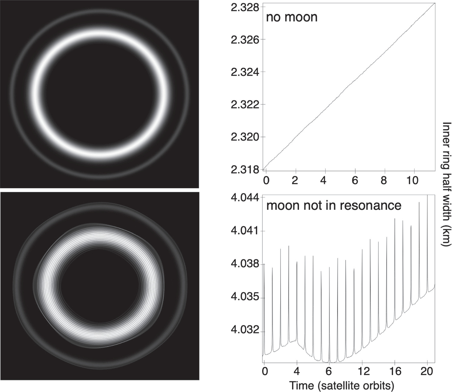
Figure 1. Demonstration of the effect of there being no satellite or a satellite outside of resonance for a Chariklo-like ring system. These plots are from simulations 1 and 2 in Table 2 (top and bottom, respectively). The left column contains visual representations of the distribution of ring material at the end of the simulation: black to white represents model optical depths 0–1. The right column shows the evolution of the width of the inner ring throughout the simulation. In both cases, the ring material was not confined. Note: the radial scale in the left column is exaggerated by a factor of five for better visualization. The widths are calculated from binned data. The meter-scale jumps in ring width in the lower right plot are due to single particles being included or excluded when binning over the ring to plot the width.
Download figure:
Standard image High-resolution imageA satellite in resonance with the rings acted to confine the particles to km-level widths over a relatively short timescale. Examples are shown in Figure 2 for a satellite in both an inner and outer mean-motion resonance (MMR) with the rings. In these cases, the inner ring was on a first-order MMR with the satellite and another resonance was near the inner part of the outer ring. The effects of the satellite perturbation are apparent in both rings as azimuthal and radial variations in the distributions of particles. We note that the effect of a satellite in an interior resonance can be considered dynamically similar to that of one in an exterior resonance, or that of a non-axisymmetric nucleus that is in a rotational resonance with the rings (as considered by Sicardy et al. 2019).

Figure 2. Demonstration of the effect of a satellite in resonance for a Chariklo-like ring system. These plots are from simulations 3 and 4 in Table 2 (top and bottom, respectively). The left column contains visual representations of the distribution of ring material at the end of the simulation: black to white represents model optical depths 0–1. The right column shows the evolution of the width of the inner ring throughout the simulation. A single satellite, in orbital resonance either interior or exterior to rings, confined the ring material to widths of a few km. Azimuthal variations are apparent. The bottom plot is somewhat similar to Chariklo's known ring system; however, the ring was still shrinking at the time the simulation was halted. Note: the radial scale in the left column is exaggerated by a factor of five for better visualization. The widths are calculated from binned data. The meter-scale jumps in ring width in the lower right plot are due to single particles being included or excluded when binning over the ring to plot the width.
Download figure:
Standard image High-resolution image3.1.2. Satellite Mass and Ring Optical Depth
To explore the effect of the satellite mass, as well as a broader range of ring-particle characteristics, we carried out simulations 5–9 in Table 2 for the inner ring only. For these simulations, we fixed the satellite location at the 4:5 MMR. This resonance was chosen based on the initial simulations, because it confined ring material at the approximate locations of C1R and C2R within a reasonable timescale. Placing the satellite in other resonances will change the strength and number of perturbations, resulting in different ring characteristics and timelines for confinement (e.g., Figure 2). We explored a range of satellite masses from 7.5 × 10¹² to 6 × 10¹³ kg (∼10−7–10−6 the mass of Chariklo) and a range of ring model optical depths from 0.02 to 0.4. Ring-particle sizes were 1–10 m in radius, following a power-law distribution with fixed index q = 3. The particle density was 0.5 g cm−3.
Figure 3 shows the ring guiding-center full width at half maximum (FWHM) over time of a subset of these simulations, for three different satellite masses and a ring of two different model optical depths. Setting an initial condition of τm = 0.4 in these simulations produced clumping of material, as well as an increased collision rate, and it slowed the computations to the point of being unreasonable. Simulations 1–4 did not demonstrate this, because particle self-gravity was not included, but here we took the more physically realistic approach of increasing particle density and reducing the initial model optical depths. See Section 4 for further discussion.
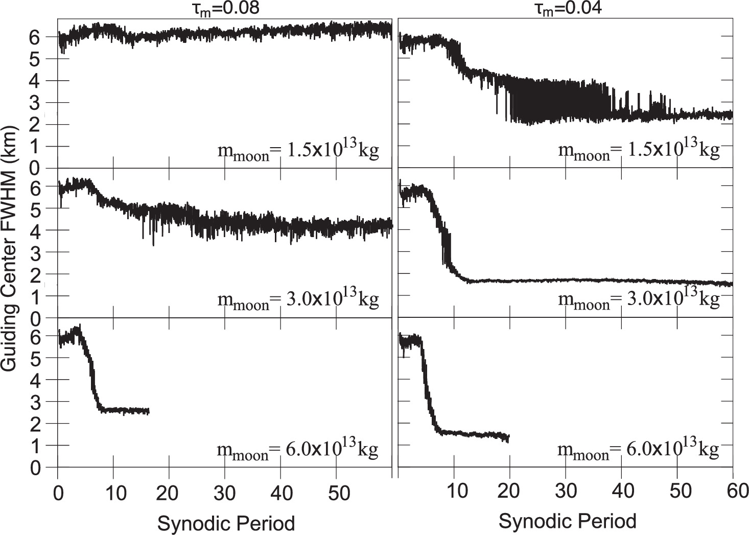
Figure 3. The effect of satellite mass on the FWHM of the ring guiding-center core, from a subset of simulations 6 and 8 in Table 2. The initial conditions consider material with two different optical depths, τm = 0.08 (left) and τm = 0.04 (right). The mass of the satellite is given for each panel as mmoon. The higher optical depth required a more massive moon for confinement. The middle right simulation produced a ring similar in width to C1R and was used to produce Figure 4. We note that the simulations in the bottom panels were halted once they reached equilibrium, while in the upper panels they were continued.
Download figure:
Standard image High-resolution imageFrom Figure 3, satellites with the lowest mass (1.5 × 10¹³ kg) maintained but did not confine the ring to the observed widths. A satellite with a slightly higher mass contracted the ring to the few-km widths observed for C1R. However, as optical depth increased, the mass of the satellite required for confinement also increased. Satellites with higher mass contracted the ring even further, to the scale of a single km.
The width of the simulated ring from the middle right panel in Figure 3 is shown in Figure 4. This plot demonstrates that the actual ring width varied over azimuth. The azimuthal width variations in this simulation were approximately two km.
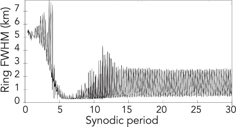
Figure 4. FWHM of the simulated ring vs. time for simulation 6 with satellite mass 3 × 10¹³ kg from Table 2, which corresponds to the middle right panel in Figure 3. This plot demonstrates that the ring width varied by a few km azimuthally.
Download figure:
Standard image High-resolution imageIn Figure 5, we have combined the results from simulations 5–9 to roughly map ring confinement as a function of satellite mass and initial optical depth of the inner ring. Material is defined to be confined with a visual inspection of the density of guiding centers over the course of the simulation. Satellite mass and ring optical depth were positively correlated, in an approximately linear relationship, in terms of confining material to the few-km width observed for Chariklo's inner ring. In addition, tighter confinement occurs for simulations that have lower initial optical depths (and thus lower initial collisional rates).

Figure 5. Confinement of ring material as a function of satellite mass and ring optical depth for simulations 5–9 in Table 2. Yellow to blue coloration represents the guiding-center width of the inner ring, and data points with black centers are confined when the simulations reach steady state. A gray line represents a roughly linear divide, above which ring material is confined and below which it is not.
Download figure:
Standard image High-resolution image3.2. Accretion Simulations
We next explored the impact of the shepherd-moon wakes on accretion. The confinement mechanism from single-sided shepherding produces wakes with a significantly higher density than the general ring material, where particles can easily form clumps or gravitationally bound moonlets. Lewis & Stewart (2005) found that material leaving the satellite wakes in simulations of the Encke gap formed extended gravity wakes. While this mechanism could enhance accretion, the dynamics of the satellite wakes produces regions of rarefaction in addition to the compression. This occurs when the perturbed streamlines separate. Our simulations addressed two hypotheses relating to accretion in the Chariklo system: (i) particles that are not sufficiently bound together will shear out, and (ii) collisional interactions between the wakes and the moonlets will cause more erosion than additional accretion.
We ran two simulations with parameters that favored accretion: one used the standard hard-sphere model and the other used the soft-sphere model, following Section 2.2.1. The satellite was 3 × 10¹³ kg in the 4:5 MMR, the initial ring optical depth was 0.1, and the particle density was 0.5 g cm−3 (Table 2). To promote accretion, these simulations considered a smaller range of particle sizes (1–1.1 m in radius with q = 3) and Chariklo had a smaller mass (5 × 10¹⁸ kg). Using the size from Morgado et al. (2021), this mass corresponds to a density of 0.62 g cm−3 for Chariklo. These parameters give a scaled Hill radius of 1.27, which is significantly larger than the value of 1.1 found to lead to accretion in previous ring studies (see Section 3.2 of Michikoshi & Kokubo (2017), for references). In other words, the ring was well outside the classical Roche limit in these simulations.
The accretion-testing simulations were run for just over 30 orbits, long enough for the resonant satellite wakes to form and for self-gravity to begin the process of accreting particles. We found and tracked moonlets from the time of their formation to when they fell apart or the end of the simulation, following the method in Section 2.3. Results from the simulations at three specific time steps are shown in Figure 6. Figures 7–9 contain close-ups of a selection of the moonlets detected during these time steps.
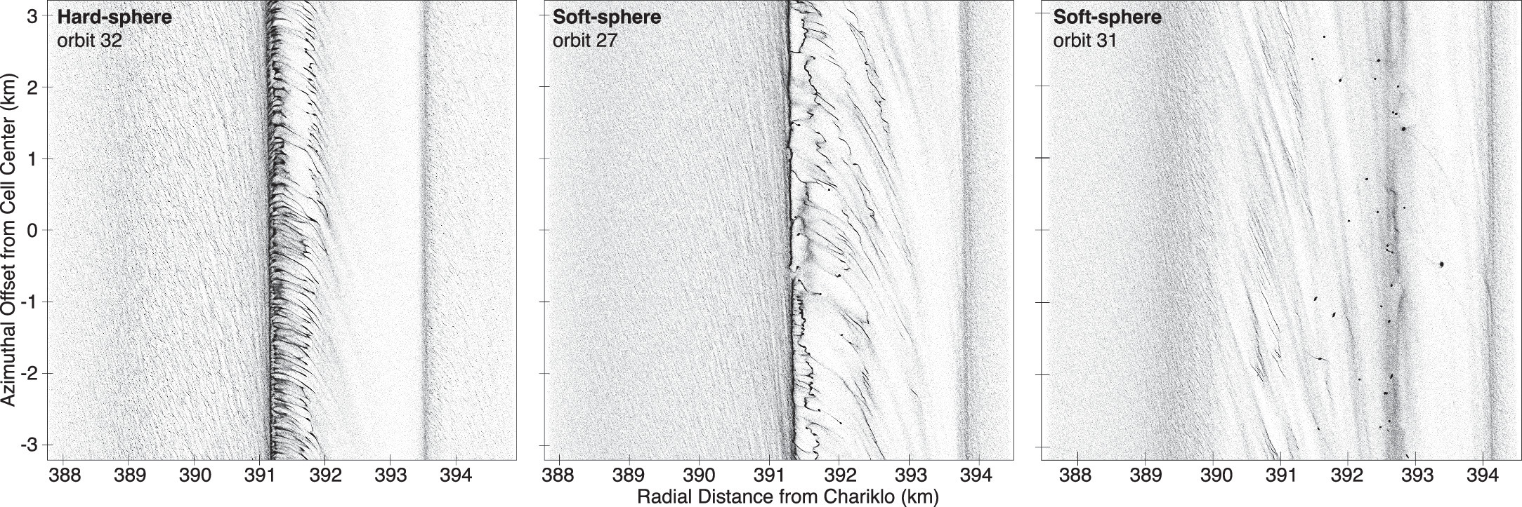
Figure 6. Full-cell snapshots of the accretion simulations. Each simulated particle is plotted as a black point. The panels are (left) the 32nd orbit from the hard-sphere simulation, (middle) the 27th orbit of the soft-sphere simulation, and (right) the 31st orbit of the soft-sphere simulation. Accretion does not form stable moonlets in the hard-sphere simulations, whereas it does in the soft sphere. By the end of the soft-sphere simulation, much of the material had accreted into ∼30 moonlets and the optical depth of the wake was greatly reduced.
Download figure:
Standard image High-resolution image
Figure 7. Snapshot from the 32nd orbit of the hard-sphere, accretion simulation. Each simulated particle is plotted as a black point. On the right is a slice through the simulation cell (the left panel in Figure 6). On the left are close-ups of the two longest-lived moonlets detected in this simulation, which lasted less than one orbit before shearing out. The moonlets are plotted in the same colors in the right panel, to indicate their locations.
Download figure:
Standard image High-resolution imageFigure 7 shows the state of the hard-sphere simulation during the 32nd orbit, in which the density wakes were easily visible and there were two moonlets. Moonlets formed as clumps of material fell out of the passing satellite wake, where densities were elevated; however, the material was only tenuously bound and sheared out with even small perturbations. The top moonlet lasted the longest of any in this simulation: no moonlets were stable longer than half an orbital period.
Figure 8 shows the state of the soft-sphere simulation early in the 27th orbit. As with the hard-sphere simulation, material came out of the satellite wake in clumps. Unlike the hard-sphere simulation, the highest-density clumps formed moonlets that were stable for many orbits. Figure 8 highlights nine of the more than 40 moonlets present at this time, most of which display tails of sheared material.

Figure 8. Snapshot from the 27th orbit of the soft-sphere, accretion simulation. Each simulated particle is plotted as a black point. On the right is a slice through the simulation cell (the middle panel in Figure 6). The density wakes are visible but are less apparent than in the hard-sphere simulation because more material had accreted into moonlets. On the left are close-ups of a subset of the moonlets detected during this step. The examples here are representative of the more than 40 moonlets identified at this time. The moonlets are plotted in the same colors in the right panel, to indicate their locations.
Download figure:
Standard image High-resolution imageFigure 9 shows the soft-sphere simulation near the beginning of the 31st orbit. At this point, a reasonably large fraction of the ring material was contained in just over 30 moonlets. The satellite wake was not as defined because the effective optical depth had been dramatically reduced. The state of the ring was similar to the oligarchic growth phase seen in planetary-formation simulations. The moonlets also had crossing orbits, so they could collide. Such collisions were rare and more energetic than earlier in the simulation, although the collisions at this time were generally not destructive.
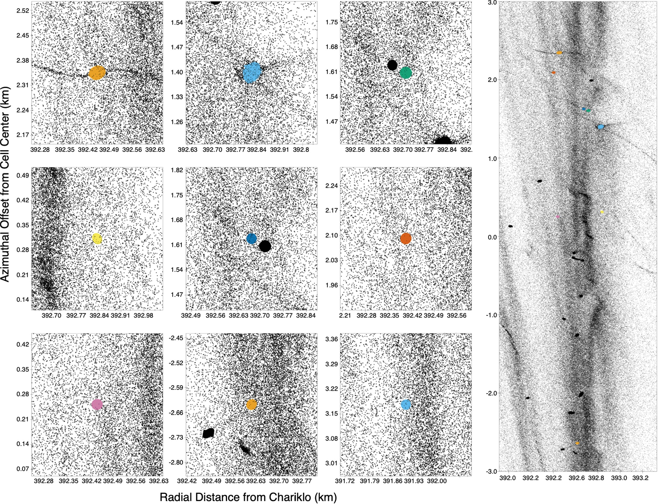
Figure 9. Snapshot from four orbits later than Figure 8 of a soft-sphere, accretion simulation. Each simulated particle is plotted as a black point. On the right is a slice through the simulation cell (the right panel in Figure 6). On the left are close-ups of some of the moonlets detected during this step. The top left and top center moonlets were the longest-living ones in the simulation. The moonlets are plotted in the same colors in the right panel, to indicate their locations.
Download figure:
Standard image High-resolution imageA plot of the number of moonlets detected along with the numbers of particles in those moonlets as a function of time for both the hard- and soft-sphere simulations is shown in Figure 10. To remove any "false positives" in the wake peaks, only clumps of particles that survived for at least one-third of an orbit were counted. In both simulations, the number of moonlets varied throughout an orbital period because the satellite wake created and destroyed clumps of material. No moonlets survived long-term in the hard-sphere simulation. Indeed, when the criteria to rule out false positives was increased to one-half of an orbit, there was never more than one moonlet present at any time in the hard-sphere simulation. The oscillations were created by the fact that moonlets formed as material dropped out of the wake peak, then fell apart because of various collisions with other ring material over the course of the next orbit.
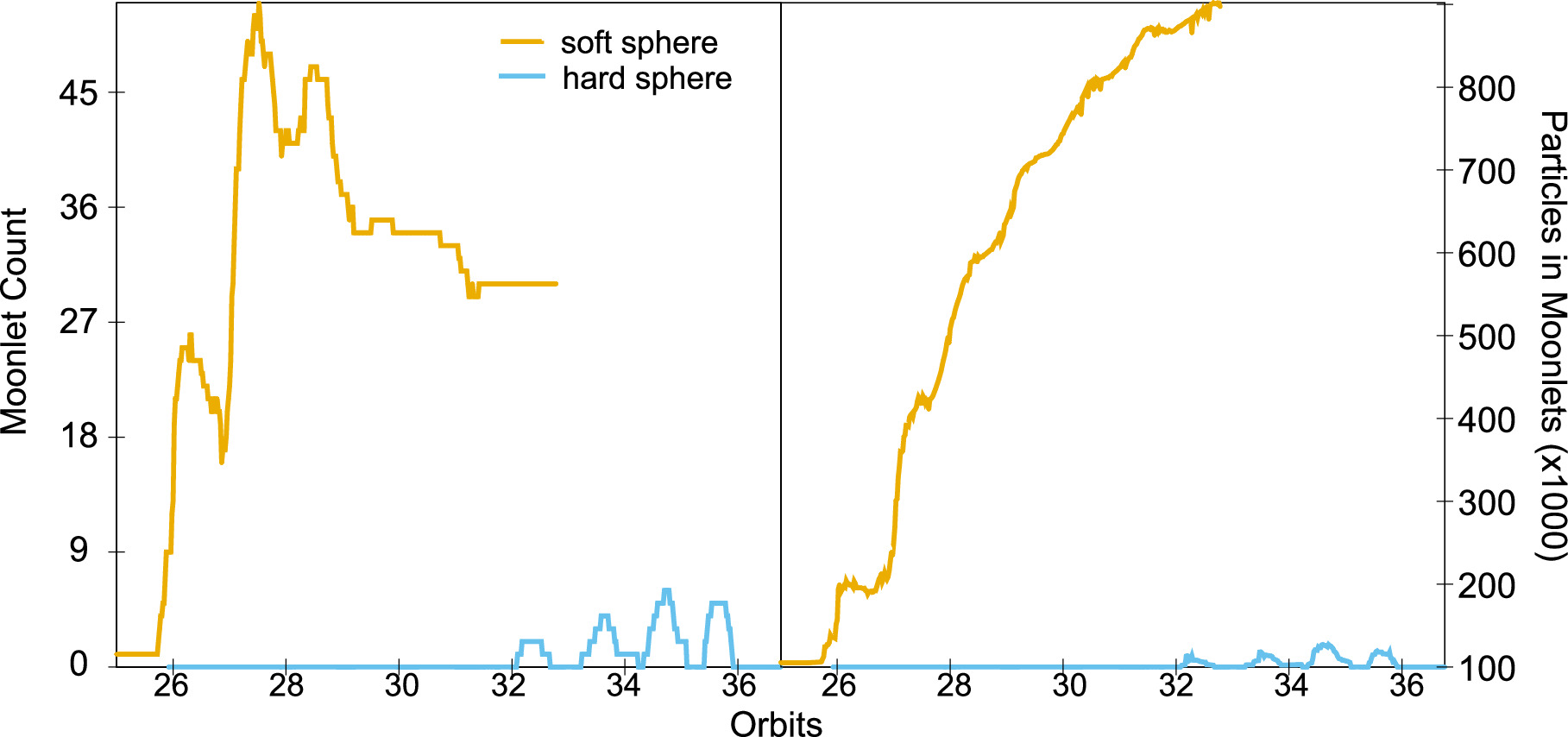
Figure 10. (left) Number of moonlets detected and (right) number of particles in those moonlets vs. time for the accretion simulations. The hard-sphere simulation is plotted in teal, and the soft-sphere simulation is plotted in dark yellow. Moonlets were not sustained in the hard-sphere simulations, and for the soft-sphere simulations, particles continued accreting into moonlets. The plots start at the orbit in which the first long-lived moonlet was detected. The periodicity of the satellite wake is apparent as moonlet creation and destruction on suborbital timescales, in particular in the hard-sphere simulation. Only clumps that lasted at least one-third of an orbit were included to remove any false positives.
Download figure:
Standard image High-resolution imageIn the soft-sphere simulation, the number of moonlets increased drastically to nearly 50 before leveling out to roughly 30 stable moonlets at the end of the simulation. These simulations included roughly 2.5 million particles with a narrow size distribution. In roughly 30 orbits, nearly a third of the simulation material was entrained into approximately 30 larger moonlets. The final moonlet count leveled off when the wakes no longer had sufficient material to form new moonlets and the mean intercollision time for the moonlets was large, much like in the oligarchic growth phase seen in planetary simulations.
4. Discussion
We have demonstrated that a single satellite can confine ring material at the approximate location, width, and optical depth observed for C1R at Chariklo. The dynamical mechanism that confines ring material with a shepherd moon works when the particles are in a rotational resonance with the satellite. Initial simulations of a two-ring system suggest that both C1R and C2R can be confined if both rings are in resonance with the satellite. The majority of the presented simulations consider a satellite that is interior to the rings, in a 4:5 MMR with C1R. Either an exterior or interior satellite in resonance will have the same effect. The dynamical mechanism works similarly to a gravitational anomaly that is in a rotational resonance with the rings. Unlike the giant planets, small bodies with modest topographical features or elongations may exhibit non-axisymmetric gravitational field terms that lead to strong resonances between their spin and ring particles. Sicardy et al. (2019) showed that material inside of Chariklo's corotation radius can migrate onto the nucleus, while material outside is pushed outside the 2:1 spin–orbit resonance. Chariklo's rings are cleared within the corotation radius, and they are located close to the 3:1 resonance with the spin period (Leiva et al. 2017; Ortiz et al. 2017). A satellite, a gravitational perturbation, or both could be occurring at Chariklo.
Our hard-sphere simulations do not easily accrete into moonlets, while the soft-sphere collisions can sweep most of the ring material into moonlets in a relatively short period of time. The soft-sphere simulations are likely nonphysical in terms of the stability of the moonlets. This is because gravitational attraction between particles that overlap is not included in the force model, as such particles push apart in the damped-spring model. However, when particles are in a clump, they do feel the attractive gravitational force of all the particles with which they do not directly overlap. The particles in the center of the moonlet clumps have nonphysically large overlaps, on the order of 50%. For moonlets with thousands of particles, there is still a reasonably large compressive force. The existence of rings implies that particles orbiting Chariklo do not accrete quickly and therefore contains information about the properties of the ring material. It is likely that the ring particles have physical properties that are somewhere between what is represented by our hard- and soft-sphere simulations.
Our simulated rings are not eccentric; they are perturbed circular rings. Figures 11 and 12 show the characteristics of epicyclic phase (φ), forced eccentricity (ef ), and guiding-center optical depth (τgc ) for one of the simulations. Figure 12 contains the characteristics throughout the full simulation, while Figure 11 shows the final orbit projected onto a circle for better visualization. The circularity of the ring is demonstrated through the circular nature of τgc as well as φ, the latter of which shows the apses at different azimuthal locations based on radial position and a sheared m = 4 perturbation in Figure 11. The black circle in Figure 11 allows comparison of the distributions of these characteristics with respect to the location of the resonance itself. There is more material toward the location of the satellite from this resonance (here interior), as shown in the plot of τgc . If the proposed 3:1 spin–orbit resonance acts similarly, there may likewise be an offset distribution of ring material. We note that Chariklo is known to be a non-axisymmetric body (e.g., Morgado et al. 2021), while our model considers both the nucleus and the satellite to be point sources. The effects of a non-axisymmetric nucleus will be an area for future work, but the timescales for those gravitational effects are likely to be longer than the tens of orbits in which we find that perturbations from a satellite act on the ring particles.
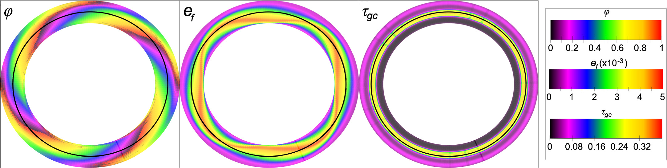
Figure 11. Characteristics within the simulated ring at steady state: epicyclic phase (φ), forced eccentricity (ef ), and guiding-center optical depth (τgc ). The color-scale legend provides quantification for each of the parameters from low (indigo) to high (red), and the radial scale has been exaggerated for better visualization. The circularity of the ring is demonstrated in the plots of τgc and φ. Perturbations to the ring material are particularly evident in ef . For reference, a solid black line is plotted at the 4:5 MMR with the satellite. This example plot is provided for the hard-sphere accretion simulation number 10 in Table 2: this figure is a circular projection of the data from the final orbit shown on the far right side of Figure 12.
Download figure:
Standard image High-resolution image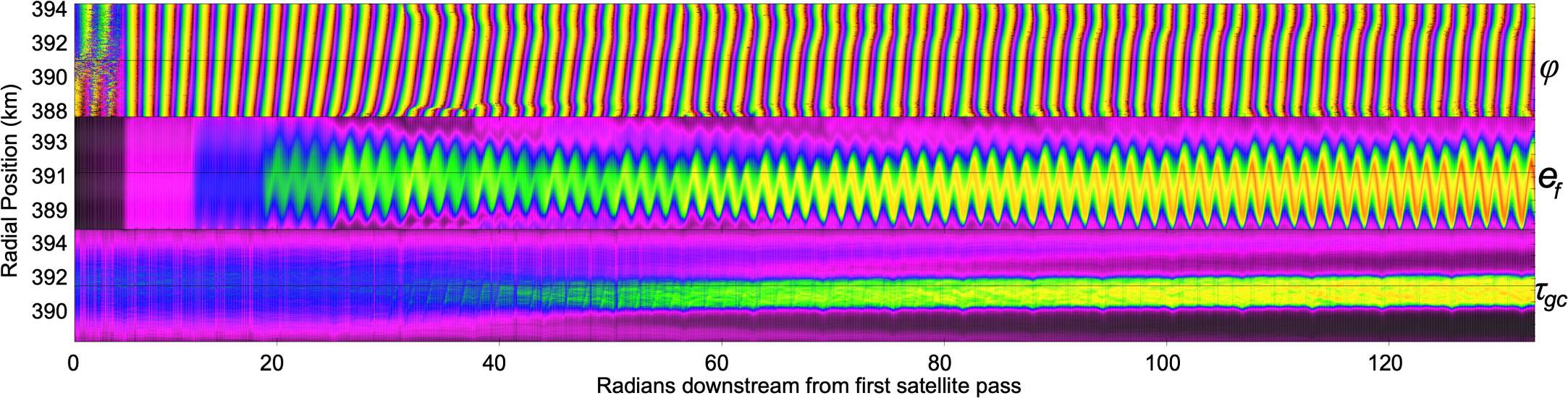
Figure 12. Characteristics of the ring throughout the hard-sphere accretion simulation number 10 in Table 2: epicyclic phase (φ), forced eccentricity (ef ), and guiding-center optical depth (τgc ). This plot demonstrates how these parameters vary from the initial conditions through to steady state. The color-scale legend is the same as in Figure 11. The values for the final orbit are projected into circles in Figure 11, to better visualize the properties of the ring.
Download figure:
Standard image High-resolution image
4.1. Could Chariklo Have a Satellite?
The satellite that produced the ring widths shown in Figure 4 would have a radius of ∼3 km, assuming a reasonable density of 1.5 g cm−3. Although Chariklo is not currently known to have any satellites, the existence of a few-km-sized moon at Chariklo is not unrealistic. The angular size of a 2 km body at Chariklo's current distance is <0.1 mas, with the entire ring system extending ∼75 mas. Direct imaging, for example with the Hubble Space Telescope, has not been able to resolve the rings nor anything else closer than 1000 km from Chariklo's center (e.g., Bérard et al. 2017). In addition, a few binary Centaurs have been detected (e.g., Noll et al. 2006, 2008) and 50%–60% of one of the Centaur's parent TNO populations, the Plutinos, are thought to consist of tight binary systems (Di Sisto et al. 2010; Thirouin & Sheppard 2018).
4.2. Optical Depth
An important factor in the simulations and the observations is ring optical depth. Optical depth is related to both particle sizes and surface number densities: a simplistic example is that higher optical depth can be caused by a few large particles or many small particles (e.g., van de Hulst 1957). The particle size distribution is thus a key parameter for ring modeling, which is currently unknown for Chariklo.
Assuming that the apse alignment is maintained by the ring's self-gravity, Pan & Wu (2016) estimated a typical particle size of a few meters. On the other hand, Michikoshi & Kokubo (2017) argued that the Centaur rings are observable only given ring particles smaller than a meter or with the existence of shepherding satellites, otherwise the viscous spreading occurs on too short a timescale (100 yr). Analysis of dual-wavelength data (visible and red) from a stellar occultation by Morgado et al. (2021) showed no dependence of ring opacity with observational wavelength, suggesting that the particle sizes are larger than a few microns.
The simulations presented here have a minimum particle radius of 1 m. The size distributions of planetary rings are typically well-described by a power law with a differential slope that is characterized by a steep increase in the number of particles at smaller sizes. For this reason, it is impractical from a computational standpoint for ring models to consider particles at scales smaller than roughly a meter for a cell this size, artificially limiting the optical depth of systems that can be effectively simulated (or ignoring particle self-gravity, as in simulations 1–4 in Table 2). However, stellar-occultation observations are sensitive to small particles, down to submicron sizes for visible-wavelength data. Therefore, caution must be taken when comparing modeled and observed optical depths.
The optical depths reported for our simulations are geometric optical depths of the fractional area coverage, calculated by
where ri
is the radius of the ith particle and A is the area of the simulation cell in the ring plane. Observed optical depths are calculated from stellar-occultation data. Stellar occultations measure the transmission, T, of light when a star is blocked by ring material. The optical depth along the line of sight, τ0, is calculated by  , and the normal optical depth, τN, is calculated given a ring opening angle, B, by
  (for a polylayer ring, e.g., Elliot et al. 1984). Reported optical depths for Chariklo's rings, the proposed rings at Quaoar, and the recent recalculation of the characteristics of the features at Chiron have included a factor of two in this calculation,
  (Braga-Ribas et al. 2014; Bérard et al. 2017; Braga-Ribas et al. 2023; Morgado et al. 2023; Pereira et al. 2023). This factor is based on inferred physical properties of the rings, assuming that the rings are thin and the occultation optical depth is larger, by an extinction efficiency factor of two, than the area physically filled, similar to what is observed for the Uranian rings (e.g., Cuzzi 1985; Roques et al. 1987). Published values for normal optical depths for material surrounding Chiron were based on the standard calculation (Sickafoose et al. 2020, 2023). It is important to take this factor of two into consideration when comparing published ring characteristics and determining model parameters.
Here, we have used the normal optical depths for Chariklo given by Braga-Ribas et al. (2014) while not employing self-gravity, or we have used significantly lower model optical depths with reasonable particle densities. A factor-of-two increase from the published optical depth for C1R would be too dense for our simulations to proceed reasonably, noting again that occultations can detect much smaller particles sizes than those in our simulations—and thus model and observed optical depths need not be equivalent.
4.3. Applicability to Other Ring Systems
The model presented here could apply to other small-body ring systems. The Centaur Chiron is similar in size to Chariklo (spherical estimate of 218 ± 20 km and ellipsoidal with semi-axes of 114, 98, and 62 km; Lellouch et al. 2017; Braga-Ribas et al. 2023) with a similar rotational period (5.92 hr; Marcialis & Buratti 1993), and its orbit ranges from 8.5 to 19 au. Stellar occultations in the early 1990s revealed an asymmetric dust coma at Chiron as well as narrow jets (Elliot et al. 1995; Bus et al. 1996). A combination of stellar occultations, rotational light curves, and long-term photometric and spectroscopic variations have been used to support the idea of a two-ring system with additional surrounding material (Ortiz et al. 2015; Ruprecht et al. 2015; Sickafoose et al. 2020). The proposed Chiron rings are at 300 and 309 km, are 2.5–4.5 km in width, and vary azimuthally in width by 1.5 km (inner ring) and 0.5 km (outer ring) (Sickafoose et al. 2020). However, the most recent occultation observations suggest that the situation is not as simple as a stable, two-ring system (Ortiz et al. 2023; Sickafoose et al. 2023). Further observations are needed to better characterize material around Chiron, but the demonstrated applicability of our simulations for Chariklo suggests that they could also be relevant for any stable rings at Chiron.
Haumea was the second small body with a confirmed ring system (Ortiz et al. 2017). Unlike Chariklo and Chiron, Haumea is a large TNO with even faster rotation and known satellites: assuming a triaxial ellipsoid, the size is estimated to be 2322 × 1704 × 1026 km, its orbit ranges from 35 to 52 au, and the rotational period is 3.9 hr (Rabinowitz et al. 2006; Ortiz et al. 2017). Haumea has a collisional history, which resulted in the formation of its two satellites and more than a dozen smaller TNOs known as Haumea-family objects (e.g., Brown et al. 2007; Ragozzine & Brown 2009; Schlichting & Sari 2009; Leinhardt et al. 2010). A single, coplanar ring was detected at Haumea, with a width of ∼70 km at a radius of ∼2287 km, which is inside the Roche limit (Ortiz et al. 2017). In size, body shape, and ring width, the Haumea system is different from Chariklo and Chiron. Although the known satellites could suggest that Haumea is a good candidate for our simulations, they orbit far enough away from the ring that they do not affect it dynamically. Our simulations also specifically maintain narrow rings a few km in width, and they are thus likely to be less applicable to Haumea than to the Centaur systems.
Most recently, one or two possible rings were reported around Quaoar (Morgado et al. 2023; Pereira et al. 2023). Quaoar is a ∼1110 km diameter TNO, orbiting from 42 to 45 au, with a rotational period of either 8.84 hr (single-peaked) or 17.68 hr (double-peaked) (Trujillo & Brown 2003; Brown & Trujillo 2004; Braga-Ribas et al. 2013; Morgado et al. 2023). It is known to have one satellite, Weywot (e.g., Fraser & Brown 2010). Quaoar does not have a homogeneous ring: the majority of Quaoar stellar-occultation light curves have not detected any material or only during either ingress or egress (Morgado et al. 2023; Pereira et al. 2023). There is a wide range of reported normal optical depths, with only one significant detection having a low-error measurement where τN ⪆ 0.1 (Morgado et al. 2023; Pereira et al. 2023). The proposed rings are located at 2520 and 4057 km, with possibly all—and certainly the more distant—material being well beyond the Roche limit (Pereira et al. 2023). Quaoar is known to have a moon, Weywot, for which the more distant ring is proposed to be in a 6:1 MMR, considering the double-peaked period (Morgado et al. 2023; Pereira et al. 2023). If stable rings were confirmed at Quaoar, this could be the most applicable system to model using our simulations.
5. Conclusions
We have carried out a set of N-body simulations to explore the efficacy of a single satellite as a confinement mechanism for Chariklo-like rings. We find that ring material spreads in the control case of no perturber in the system. Ring material also spreads if there is a satellite in the system but it is not in a mean-motion resonance with the rings. A satellite in resonance with the ring(s) can confine the material: an exterior resonant satellite (6:5 MMR) or an interior one (4:5 MMR) both work well. We further find that (i) a low-mass satellite is insufficient to confine ring material, (ii) a satellite of sufficient mass confines the ring to the observed scale of a few km in width, (iii) as ring optical depth increases, the satellite mass must also increase to allow confinement, and (iv) more massive satellites can produce even thinner rings than those observed.
The midrange satellite mass in our simulations (3 × 10¹³ kg) confines a ring to a width of a few kilometers and exhibits azimuthal width variations on the order of a few km, which are similar in scale to the observed properties of C1R. Such a satellite would be a few km in radius, which is below the current direct-detection limits in the Chariklo system. These results used model optical depth of τm = 0.04 with particles of density 0.5 g cm−3 from 1 to 10 m in radius. The simulation phase space explored here is not exhaustive, but it does provide representative conditions under which a Chariklo-like ring can be maintained. For example, more work is needed to determine if there is a preferred satellite MMR to best match the observations. We note that the dynamical mechanism explored here works similarly to a topographical surface feature that is in a rotational resonance with the rings: either or both of these processes could be occurring at Chariklo.
A shepherd satellite also provides a mechanism to both create and destroy clumps of ring material. To investigate the behavior of material that is possibly located outside the Roche limit, we conducted simulations that were favorable to accretion for hard- and soft-sphere models. For hard-sphere simulations, we find that ring material clumps as a result of the satellite density wakes but shears out on timescales of less than one orbit. For soft-sphere simulations, many moonlets were formed. After approximately 30 orbits, most of the material accreted into moonlets and the optical depth of the ring is greatly decreased. It is likely that Chariklo's ring particles have physical properties that are somewhere between what was represented by our hard- and soft-sphere simulations. An area of future work is to explore the properties of model particles in order to place better constraints on the physical properties of ring particles at Chariklo. In addition, we plan to look into how our model could be modified to investigate the proposed 3:1 spin–orbit resonance of a non-axisymmetric body (e.g., as proposed by Sicardy et al. 2019).
Acknowledgments
This work was supported by National Science Foundation (NSF) Astronomy and Astrophysics Research Grants award number 2206306.