

Do Consumption-Based Asset Pricing Models Explain the Dynamics of Stock Market Returns?

1
Faculty of Economics, Downing College, University of Cambridge, Cambridge CB2 1TN, UK
2
Faculty of Economics, Trinity College, University of Cambridge, Cambridge CB2 1TN, UK
*
Author to whom correspondence should be addressed.
J. Risk Financial Manag. 2024, 17(2), 71; https://doi.org/10.3390/jrfm17020071
Submission received: 20 December 2023
/
Revised: 31 January 2024
/
Accepted: 6 February 2024
/
Published: 11 February 2024
(This article belongs to the Special Issue Advanced Studies in Empirical Asset Pricing)
Abstract
:We show that three prominent consumption-based asset pricing models—the Bansal–Yaron, Campbell–Cochrane and Cecchetti–Lam–Mark models—cannot explain the dynamic properties of stock market returns. We show this by estimating these models with GMM, deriving ex-ante expected returns from them and then testing whether the difference between realised and expected returns is a martingale difference sequence, which it is not. Mincer–Zarnowitz regressions show that the models’ out-of-sample expected returns are systematically biased. Furthermore, semi-parametric tests of whether the models’ state variables are consistent with the degree of own-history predictability in stock returns suggest that only the Campbell–Cochrane habit variable may be able to explain return predictability, although the evidence on this is mixed.
Keywords:
performance of asset pricing models; consumption-based asset pricing models; serial correlation; predictability; martingale difference sequence; variance ratio; quantilogram; rescaled range; power spectrum; Mincer–Zarnowitz regression; MIDASJEL Classification:
C52; C58; G121. Introduction
Three prominent consumption-based asset pricing models—the Bansal–Yaron, Campbell–Cochrane and Cecchetti–Lam–Mark models—cannot explain the dynamics of US market return. The Bansal–Yaron and Campbell–Cochrane models are designed to explain the level of stock market returns, in particular to simultaneously resolve the equity premium and risk-free rate puzzles. Yet, whether these models can explain the degree of predictability in stock returns is of interest, too, especially if investors want to time or beat the market. In this sense, the dynamics (second moment) of returns are important separately to their level (first moment). This is recognised in Cecchetti et al. (1990). The Cecchetti–Lam–Mark model was developed specifically to explain return dynamics, rather than to price assets per se.
Our first tests of whether the three models can explain return dynamics amount to testing whether the difference between the model-implied ex ante expected market return and the realised market return—the residual—is a martingale difference sequence (MDS). Since the residuals are not MDS, there is some part of the dynamics of realised returns not captured by the models. To construct the expected returns and residuals, we first estimate the models by GMM. Our testing procedures account for this estimation step.
We base our tests of the null that the residuals are MDS on serial correlation, quantile hits, the rescaled range and the generalised spectrum of Hong (1999). The asymptotic distribution of the serial correlation and generalised spectrum-based tests accounts for the initial estimation step, while we use a bootstrap procedure to account for the estimation step in the quantile hits and rescaled range-based tests. We use a battery of tests since tests of the MDS null can suffer locally low power against certain alternatives (Poterba and Summers 1988).
Our finding that none of the three models’ residuals are MDS is robust to the empirical choices we make. It does not matter whether we use the optimal GMM weight matrix, or the identity matrix; whether we use size/book-to-market or industry portfolios to estimate the models; or whether we use quarterly instead of annual data. The only apparent hope comes from estimating the Cecchetti–Lam–Mark model using size/book-to-market portfolios and the identity GMM weight matrix at quarterly frequency. However, using a quarterly sample offers a much larger number of observations and allows for us to consider the robustness of our results over time by splitting the sample into two equal-length sub-samples. In doing this, we clearly reject the null that the Cecchetti–Lam–Mark residuals are MDS in both sub-samples.
As a further test, we use Mincer–Zarnowitz regressions (Mincer and Zarnowitz 1969) to test whether out-of-sample model-generated expected returns are systematically biased, finding that they are. Rational expectations would rule out such systematic bias. We find significant evidence of systematic bias in Bansal–Yaron expected returns. While the null of unbiased expected returns is not rejected for the Campbell–Cochrane and Cecchetti–Lam–Mark models in the main results which estimate the models using the optimal GMM weight matrix, size/book-to-market portfolios and annual data, there is a negative correlation between the expected returns and actual returns. In any case, the null of unbiasedness is rejected in all of the robustness check cases.
In each of the robustness check cases, we consider only models that provide credible expected returns. Many of the robustness check specifications do not offer plausible expected returns series. This is less surprising than it might seem given the difficulties in identifying the parameters of asset pricing models (Cheng et al. 2022). There is no point checking the second moment of a model that fits poorly in terms of the first moment, as one would not use it to price assets anyway. Moreover, the centred second moment (e.g., serial correlation coefficient) is a function of the first moment.
We also consider semi-parametric tests of whether the degree of predictability in returns is consistent with the state variables of the three models being correctly specified. Unlike residual-based tests, these tests do not depend on the functional form of the stochastic discount factor being correctly specified. They require only that the state variables be correctly specified.
Our first state-variable test is an adaptation of the Huang and Zhou (2017) test. We test whether from a predictive regression of returns on their lagged values exceeds a theoretical upper bound, . depends on the state variables of the stochastic discount factor (i.e., the state variables which explain stock returns).
Our second state-variable test comes from the Merton (1973) intertemporal CAPM (ICAPM). Merton shows that, if the ICAPM holds (for any risk-averse von Neumann–Morgenstern utility function), returns at , can be predicted by , the variance of conditional on information at t, and , the time-t conditional covariance of and the state variables describing the investment opportunity set, . In all of the three models, all the information required to compute is contained in some potentially non-linear function of . We therefore test whether some non-linear function of the state variables at t can predict returns once is accounted for, using a MIDAS approach to estimate . The null is that the non-linear function of cannot predict once is accounted for.
The Bansal–Yaron state variables cannot explain the predictability of returns. We find statistically significant excess predictability ( significantly greater than ) at four out of nine horizons using annual data and six out of nine horizons using quarterly data. The MIDAS-based test also fails to reject in favour of the Bansal–Yaron state variables using either annual or quarterly data.
While there is superficially more hope for the Cecchetti–Lam–Mark model state variable, this turns out not to be robust. There is statistically significant excess predictability at only one of the nine horizons considered for the Cecchetti–Lam–Mark state variable in our main results using both annual and quarterly data. However, there are many violations in each sub-sample when we split the sample into two equal-length sub-samples, and the ability of the Cecchetti–Lam–Mark state variable to explain return predictability is not robust over time. Moreover, the MIDAS-based test fails to reject in favour of the Cecchetti–Lam–Mark state variable using either annual or quarterly data.
The only model whose state variable may explain the predictability of returns is the Campbell–Cochrane model. With annual data, the MIDAS-based test rejects in favour of the Campbell–Cochrane state variable, but there is evidence of significant excess predictability. The same is true with quarterly data. Overall, the picture is mixed, since the two state variable-based tests lead to opposite conclusions.
Apart from the question of how well these models explain the dynamics of asset returns being interesting in its own right, testing this property leads us naturally to residual-based testing. This is a standard time-series specification test, although not one that is commonly used in the context of consumption-based asset pricing models. In this setting, GMM estimation and an accompanying J-test is more common. The advantage of testing the residuals, in this case from the market return, is that it allows for us to test models which are estimated in “stages”—i.e., where the estimation is not performed in one single GMM implementation. Both the Campbell–Cochrane and Cecchetti–Lam–Mark models are estimated in stages in this way.
We study the Bansal–Yaron and Campbell–Cochrane models as they are the primary textbook adaptations of the standard constant relative risk aversion (CRRA) preference model designed to simultaneously explain the equity premium (Mehra and Prescott 1985) and risk-free rate (Weil 1989) puzzles (see, e.g., Campbell 2018; Linton 2019). Assuming a standard endowment economy with a representative investor who has CRRA preferences, the observed difference between stock returns and low-risk bond yields requires extremely high levels of risk aversion to explain. This is the equity premium puzzle. The risk-free rate puzzle compounds the equity premium puzzle. If CRRA investors are indeed as risk-averse as they would need to be to justify the equity premium, low-risk bond yields are far too low. As a result, researchers such as Bansal and Yaron (2004) and Campbell and Cochrane (1999) have sought to modify the standard CRRA set-up in order to account for these puzzles. In terms of explaining the equity premium and risk-free rate puzzles simultaneously, these models perform reasonably well. But they are yet to be examined in terms of their ability to capture the predictability of stock returns in any great detail.
Huang and Zhou (2017) present the main study of how well the Bansal–Yaron and Campbell–Cochrane models explain return predictability. They develop the bound test described above, but in the context of one-step-ahead predictability of market return with respect to several well-known predictors (the book-to-market ratio, term spread, , investment-to-capital ratio, new-orders-to-shipments ratio, output gap and credit expansion).1 Huang and Zhou (2017) use Constantinides and Ghosh’s (2011) inversion of the Bansal–Yaron model which renders the state variables observable. For the Campbell–Cochrane model, the state variable is unobserved and Huang and Zhou (2017) extract it as per Campbell and Cochrane’s (1999) calibration. They do not estimate the model first, but condition on the extracted state variable. Huang and Zhou (2017) show that the degree of predictability in the market return is greater than can be explained by Bansal–Yaron and Campbell–Cochrane model state variables.
Our residual-based approach is potentially more powerful since it can detect situations where the asset pricing model suggests too little predictability. In addition, our residual-based tests have the advantage of accounting explicitly for any initial estimation of the model or its state variables. While the Bansal–Yaron model can be inverted so that its state variables are a function of observables, this inversion is not generally possible for other asset pricing models (e.g., the Campbell–Cochrane model).
Kruttli (2022) focuses on the value of consumption-based asset pricing models to investors, rather than their explanatory power per se, and studies whether using the constraints implied by the Bansal–Yaron and Campbell–Cochrane models improve the performance of regressions forecasting excess stock returns (the market risk premium). In Kruttli (2022), a Bayesian forecasting model is used and the performance of models is compared using priors derived from the Bansal–Yaron and Campbell–Cochrane models to models using priors based on the historical average. When constraining the forecast equity premium to be non-negative, the model-based priors from the Campbell–Cochrane model improve forecasting performance, but the priors from the Bansal–Yaron model do not. However, when removing the non-negativity constraint, this result is reversed.
There has been little recent work on explaining stock return dynamics in the context of consumption-based asset pricing models. Kandel and Stambaugh (1989) propose a model with a representative CRRA investor and where consumption growth is lognormally distributed with time-varying mean and variance. The mean and variance of consumption growth follow a nine-state Markov switching process and exhibit positive serial correlation. Kandel and Stambaugh’s (1989) calibration exercise shows that the model produces the “U”-shaped autocorrelation function observed in stock returns. However, the model is not able to replicate the observed pattern of small positive autocorrelations at short horizons followed by larger negative autocorrelations at longer horizons. Kandel and Stambaugh (1989) speculate that this is because their model is overly restrictive. In particular, current news only affects the conditional distribution of consumption one period in the future. Nonetheless, their model broadly matches the observed pattern of autocorrelations at horizons greater than 12 months.
Cecchetti et al. (1990) use a similar specification to that of Kandel and Stambaugh (1989). Cecchetti et al. (1990) use a Markov switching log endowment level and a more parsimonious two-state specification. They find that popular measures of serial correlation always lie within a 60% confidence interval of data simulated from the model. The Cecchetti et al. (1990) model has the same problem of not being able to generate negative autocorrelations at short horizons as the Kandel and Stambaugh (1989) model.
We update the Cecchetti et al. (1990) evidence in two ways. First, we formally estimate their model. This also allows for the development of asymptotic theory for the hypothesis tests used. Second, the Cecchetti et al. (1990) model rests on CRRA preferences. As discussed above, these have been much criticised on an empirical basis, in particular because of the equity premium and risk-free rate puzzles. We test more recent models that can potentially accommodate these two puzzles. However, we also include the Cecchetti–Lam–Mark model in our results as a benchmark, since it is a model explicitly designed to explain serial correlation in returns.
Other attempts have been made to explain stock return dynamics in a risk-based framework. Kim et al. (2001) proxy risk by volatility and use a volatility feedback model (where an unexpected change in volatility has an immediate impact on stock prices) with volatility following a two-state Markov switching process. Risk adjusting returns in this way accounts for the serial correlation observed in returns. We focus on consumption-based models, which micro-found their risk factors from the start, rather than more ad hoc risk adjustments.
Barroso et al. (2017) consider how conditional predictability of the short-run equity premium varies with economic and risk conditions.2 They model the equity risk premium as a function of economic state variables. The extent to which these state variables forecast both equity risk premium and consumption growth varies with time. When a state variable predicts consumption growth more strongly, it also contributes more to equity premium. This is consistent with the intertemporal CAPM (Barroso et al. 2017). A consumption-based asset pricing model is capable of explaining short-term conditional predictability, although no specific specification is tested.
Lansing et al. (2022) also consider more generally the extent to which a consumption-based asset pricing framework can justify excess return predictability. They find that some measure of fundamentals almost always has predictive power, while an irrationality proxy only has predictive power in samples including the Great Recession. Lee et al. (2020) show that incorporating the constraint implied by the consumption CAPM to a maximum entropy forecasting model for excess returns improves the model’s ability to capture non-linear return predictability.
This paper proceeds as follows. Section 2 outlines the three asset pricing models tested and their estimation. Section 3 discusses the tests we use. Section 4 briefly describes the data and reports the estimation of asset pricing models. Section 5 presents our empirical results regarding the predictability of model residuals and Section 6 contains our robustness analysis. Section 7 concludes the work.
2. Asset Pricing Models
2.1. Bansal–Yaron Model
The Bansal and Yaron (2004) model is described as follows:
where is the representative investor’s value function, the subjective discount factor, the risk aversion coefficient, the elasticity of intertemporal substitution (), the consumption, the dividends, the expectation conditional on information at time t, and lower-case variables denote logs of upper-case variables.
The model has three key ingredients. First, it has recursive preferences (1) à la Epstein and Zin (1989) and Weil (1989). These allow and risk aversion to differ, unlike standard CRRA preferences. This is an advantage: risk aversion and intertemporal substitution are different concepts. reflects the extent to which consumers are willing to smooth certain consumption through time, while risk aversion relates to the extent to which consumers are willing to smooth consumption across uncertain states of nature (Cochrane 2008).
Second, consumption growth (3) has a small predictable component (the long-run risk, ). Consumption news in the present affects expectations of future consumption growth, increasing the impact of current consumption news on long-run consumption and therefore the difference between present discounted values (PDVs) of dividend streams which drives returns.
Third, there is time-varying economic volatility (5) in consumption growth. This reflects time-varying economic uncertainty and is a further source of investor uncertainty and risk.
In the Bansal and Yaron (2004) calibration, the model justifies the equity premium, risk-free rate and the volatilities of the market return, risk-free rate and the price–dividend ratio.
When Constantinides and Ghosh (2011) estimate the Bansal–Yaron model by GMM, the results are mixed. Simulating through the model with the estimated parameter values, the model is able to justify the market return in all specifications considered. The mean risk-free rate can be a little high, although this too is justified when the model is estimated using the identity weight matrix. Meanwhile, the J-statistic p-value is less than 0.03 in all specifications considered. However, the estimated model still generates reasonable market returns in Constantinides and Ghosh’s (2011) simulations and the model may therefore still be of interest from an asset pricing point of view.
To estimate the model, Constantinides and Ghosh (2011) show that the log-linearised version of the Bansal–Yaron model can be inverted, allowing for the unobserved state variables to be written as a linear combination of observables as follows:
where are functions of Bansal–Yaron model parameters, as detailed in Appendix A.1, and the (log) risk-free rate. This allows for them to express the Bansal–Yaron Euler equation for a general asset as
where is the log asset return and are functions of Bansal–Yaron model parameters, also given in Appendix A.1.
In addition, they derive eight unconditional moment restrictions for continuously compounded consumption and dividend growth, which are given in Appendix A.2. These moment conditions are derived from Bansal and Yaron’s (2004) specification of consumption and dividend growth, the long-run risk and its conditional variance.
The model has 12 parameters to estimate and we use 15 moment conditions to allow for an overidentification test. Our set of moment conditions comprises an Euler equation for each of seven assets (the market index and six size and book-to-market double sorted portfolios, taken from Kenneth French’s website) and the eight time-series restrictions.
Constantinides and Ghosh (2011) show that
where is market return and are non-linear combinations of the 12 model parameters provided in Appendix A.3. This yields a plug-in estimator of , which we use as the ex ante expected market return.
2.2. Campbell–Cochrane Model
Campbell and Cochrane’s (1999) model adds a slow-moving external habit to the standard power utility function. The representative agent’s utility function is
where is the subjective discount factor, the utility curvature and the habit level of consumption. Defining and , the habit evolves according to
where is the steady-state s, and is a sensitivity function given by
with . Campbell and Cochrane (1999) set to be equal to the first-order autocorrelation coefficient of the log market price–dividend ratio, .
Consumption and dividends satisfy
with being the first difference operator and
where indicates normally and independently and identically distributed through time.
Campbell and Cochrane (1999) calibrate their model to match the annualised unconditional equity premium using monthly US data. When given actual data, the model replicates the main movements observed in stock prices. In simulations, the model is able to justify the means and standard deviations of excess returns and the price–dividend ratio, and the existence of a short-run and long-run equity premium. Moreover, this is achieved without a risk-free rate puzzle by construction: the habit is specified such that the risk-free rate remains constant and the model is calibrated such that the log risk-free rate is equal to its sample mean.3
In Garcia et al.’s (2004) GMM estimation of the Campbell–Cochrane model, the estimated is significantly greater than zero and the significantly less than one. The J-statistic p-value exceeds 0.2, although this does condition on earlier estimates of time-series parameters in the manner described below.
We estimate the Campbell–Cochrane model using a GMM procedure similar to Garcia et al. (2004). The procedure has three steps. First, we estimate time-series parameters , and in (10) by GMM. Second, we estimate and from linear regression
Based on these estimates, we generate the series . We achieve this by initialising the series at , using the estimates of the relevant time-series moments from above and assuming an initial of two. This allows for the series to be generated as per (8) and (9).
We can then proceed to the third step: estimating preference parameters and from the following equation:
using an Euler equation for each of our seven assets. We use this new estimate of to generate a new series, and re-estimate (12) based on this new series. We iterate this procedure until the estimates of and converge. The J-statistic p-values of Garcia et al. (2004) come from their final iteration of this third step, but do not account for the initial estimation steps.
We obtain from the Campbell–Cochrane model as follows. We use the fact that , where is the price of the asset and its dividend. Iterating the Euler equation forwards, we have
when we impose the no-bubble condition
Therefore,
We estimate (14) for market return by simulation. We simulate series and according to (11). Based on these series, we compute series , and conditional on , and . We repeat this procedure 200 times, where each simulated and series is of length 100. We then compute the expectation on the right-hand side of (14) as the mean of the 200 simulated realisations of the fraction inside that expectation.
2.3. Cecchetti–Lam–Mark Model
Cecchetti et al.’s (1990) model attempts to explain return autocorrelation in a rational framework. The model is an endowment economy where the representative consumer has CRRA preferences:
Here, denotes the subjective discount factor and the coefficient of relative risk aversion. Taking (log) consumption as the appropriate endowment process,
is a first-order Markov process and . denotes a bad state, so is restricted to be less than zero.
Cecchetti et al. (1990) find that, using either risk-neutral () or risk-averse () preferences, measures of serial correlation in the observed market return always lie within a 60% confidence interval of those measures, where the confidence intervals are generated by the model. The confidence intervals come from Monte Carlo distributions of the serial correlation statistics, obtained by simulating the model. The medians of the Monte Carlo distributions of the serial correlation statistics obtained using are closer to the observed serial correlation than the medians of the distributions using , so Cecchetti et al. (1990) prefer the risk-averse specification. Cecchetti et al. (1990) measure serial correlation using variance ratios and Fama and French (1988) regression coefficients4 using annual US/S&P data over 2–10 year horizons.
There is no guarantee that this model can simultaneously explain the equity premium and risk-free rate puzzles. Given the CRRA preferences, it probably cannot. However, given the model’s success in explaining market serial correlation, it is a useful benchmark for our analysis.
We use GMM to estimate and . The moment conditions comprise an Euler equation for each of our seven assets of the form
We estimate the Markov switching endowment process by maximum likelihood following Hamilton (1989). In a slight deviation from Cecchetti et al. (1990), we estimate a Markov switching process where consumption innovation , since this is more numerically stable.
and Cecchetti et al. (1990) show that
where is a non-linear function of model parameters defined in Appendix B. Since is a binary variable and the conditional probabilities of each state are known, the expectation in (17) is straightforward to compute.
3. Methods
To test whether the asset-pricing models discussed above capture the predictability of stock returns, we note that rational expectations imply
where expectations are formed under the model in question and is unforecastable at t. If the model accurately captures return dynamics, should be MDS. If not, there is clearly something in the dynamic structure of not captured by .
We denote by the parameters in the model in question and define , to make clear the dependence of the expected returns on . We estimate (18) using plug-in estimators, , of . We base our tests on the resulting residual and denote
We consider tests of linear and non-linear predictability in as well as a rescaled range test. In each case, we adapt the test to cope with the fact that is estimated and this estimate, , is a function of a parameter vector estimated by GMM. It is well known that this estimation can both affect the limiting distribution of the statistics considered and induce serial dependence in the estimated residuals not present in the population.
In light of Poterba and Summers’s (1988) argument that tests of the MDS null can have locally low power against certain alternatives, we use a battery of tests. Different tests have different power properties against different (local) alternatives. It therefore seems prudent to cover all bases and consider several tests. This approach bears fruit. Throughout the results, there are examples where one test fails to reject while all the others reject. It is not the case that the same test keeps failing to reject.
In addition to the MDS tests, we also use Mincer–Zarnowitz regressions (Mincer and Zarnowitz 1969) to test the expected returns directly, and semi-parametric tests of whether the models’ state variables—rather than just the functional form of the SDF—are consistent with the dynamics of market return.
3.1. Linear Predictability Test
A natural place to start with testing whether or not the residuals are MDS is a test based on residuals’ autocorrelations. Since the MDS null implies that all autocorrelations are zero, it makes sense to use a test statistic that incorporates autocorrelations from more than one lag. We use a weighted correlogram of the form
where is the order serial correlation coefficient of . is a weighted sum of serial correlations. If , positive autocorrelation predominates at horizon q. is evidence that negative autocorrelation predominates at horizon q. We consider years.
We use a test of the form (19) as it is a linear transformation of the variance ratio statistic. Variance ratio is the variance of the sum of q residuals divided by q times the variance of the residuals. That is, . Since under the MDS null residuals and () are uncorrelated, the variance ratio is equal to one under the null. Cochrane (1988) show we can write , hence the connection between (19) and . Poterba and Summers (1988) and Lo and MacKinlay (1989) show variance ratio tests are generally more powerful tests of the martingale difference hypothesis than unit root and autoregressive tests. The correlogram arises as a natural choice of test statistic from the Cochrane (1988) representation of the variance ratio.
In terms of estimating , we cannot simply treat estimated residuals as if they are population residuals . The estimation of affects the limiting distribution of under the MDS null (Delgado and Velasco 2011). We therefore use Delgado and Velasco’s (2011) transformation of the residual sample serial correlations. We denote the transformed autocorrelations by . Delgado and Velasco (2011) start by standardising the autocorrelations so that they have a unit variance. To achieve this, they define matrix such that
with . To make the transformation feasible, Delgado and Velasco (2011) use Lobato et al.’s (2002) estimate of ,
where , , and ℓ is a bandwidth parameter. We use .
Delgado and Velasco (2011) rid the estimated serial correlations collected in of their dependence on by projecting them onto the derivatives of . First, we define
Then, we let and . Finally, we let
Delgado and Velasco (2011) show that
where , and denotes convergence in distribution. We notice that the projections sacrifice d degrees of freedom, so that only the first serial correlations can be transformed.
3.2. Non-Linear Predictability Test
The weighted correlogram statistic is a function of the sample autocorrelations of and therefore does not exploit the full hypothesised MDS structure of . In particular, it neglects non-linear predictability. We test for non-linear predictability using Linton and Whang’s (2007) quantilogram, which is based on the correlation of quantile hits. If is MDS, probability is in the quantile given in the quantile should remain . The quantile hits are uncorrelated. The quantilogram is a more general version of Wright’s (2000) sign tests, which focus on whichever quantile zero is in.
In our test statistic, we weight the quantilogram estimates analogously to the variance ratios. This provides
where
and is the indicator function. We evaluate (21) over the same q as in the correlograms and over a range of both extreme and moderate quantiles, namely .
We use a wild bootstrap for inference. This allows for us to account for the estimation step involved in constructing . is pre-multiplied by at each t, where and . We use Mammen’s (1993) two-point distribution for .5 Then, we use the bootstrapped residuals to extract a pseudo-sample of returns by relationship
We use to generate a new series for the market value and therefore obtain the pseudo-sample of the log price-dividend ratio, . We then re-estimate the asset pricing model parameters using the modified data, generating a pseudo-sample of expected returns and thus a (new) pseudo-sample of residuals.
The empirical distribution of the weighted quantilograms thus obtained is used for inference and the bootstrap procedure is repeated 200 times.6 We notice that our procedure conditions on consumption and dividends.
3.3. Hong–Lee Generalised Spectral Test
The Hong and Lee (2005) generalised spectral test can detect both linear and non-linear predictability. We add it to our battery of MDS tests because the known low power problems of MDS tests (Poterba and Summers 1988) mean it is useful to have additional tests. The test is based on the Hong (1999) generalised spectrum, corrected for the estimation of the parameters of the residual series in a way that yields a test statistic which has a nuisance parameter-free limiting distribution.
The test statistic is
where
is the standard Normal distribution truncated on interval , , , and
Under the MDS null and the technical conditions laid out in Hong and Lee (2005, pp. 509–10), Hong and Lee (2005) show that
3.4. Rescaled Range Test
We also consider a rescaled range test. We achieve this as the rescaled range can be more powerful than other MDS tests in the presence of long-range dependence (Lo 1991). The rescaled range is
is a consistent estimator of . Given the issue of the estimation of distorting the limiting distribution of the statistic, we conduct inference using the same wild bootstrap procedure as for the quantilogram.
3.5. Mincer–Zarnowitz Regression Test
Aside from examining the model residuals, we can also test the forecasts themselves using Mincer–Zarnowitz regression (Mincer and Zarnowitz 1969). This tests (18) in a different way to the above tests. Rather than testing whether the residuals are MDS, which is one implication of rational expectations when the models tested are correctly specified, this tests the joint null that in the Mincer–Zarnowitz regression
where is the plug-in estimate of using information only up to time t. It is evident that is an implication of (18) when the model under consideration is correctly specified. If this null is rejected, the out-of-sample expected returns are systematically biased, which is inconsistent with rational expectations.
In practice, to avoid look-ahead bias, we estimate using an expanding window ending at t to estimate . The first expanding window ends halfway through the sample, which is 1973 for the annual dataset and 1982Q1 for the quarterly dataset. This is necessary to ensure a reasonable number of observations for estimating the asset pricing model. Of course, this out-of-sample approach is potentially inefficient. It means no observations of are available for the first half of the sample and the estimates of are based on smaller samples than is the case in the whole-sample approach used in the correlogram, quantilogram and rescaled range tests above. Nonetheless, the Mincer–Zarnowitz approach forms a useful complement to the other tests seeing as it is based on the expected returns themselves, rather than the residuals.
3.6. Maximal Predictability Test
Huang and Zhou (2017) develop a Wald test of whether the predictability of excess market returns, , is too large. Predictability is measured with respect to a forecasting variable, . “Too large” is defined as too large to be consistent with , the stochastic discount factor (SDF) normalised such that , being a function of a given set of state variables .7 The test is semi-parametric in that the functional form of the SDF need not be known. The Wald statistic tests whether theoretical upper bound on implied by the state variables is exceeded by the empirical from the univariate one-step-ahead predictive regression of on .
It is straightforward to verify that this test applies almost directly to the q-step-ahead predictive regression
In this context, when bounding with , the market Sharpe ratio, the bound becomes
where
and . h is a parameter chosen by the marginal investor. We follow Cochrane and Saá-Requejo (2000) in using . This bound requires to have an elliptical distribution, which it does in all models.8
Huang and Zhou’s (2017) test exploits the asymptotic normality of standard estimators of the mean and covariance matrix of . These means and covariances, which comprise , are all that is required to calculate the empirical and its bound. We follow Huang and Zhou (2017) and estimate by GMM.
Testing whether exceeds is equivalent to a one-sided test of the null against the alternative that (Huang and Zhou 2017). The Wald statistic for this test is
This procedure can then be applied to the predictive regression Fama and French (1988) use to test for serial correlation in the market return,
albeit with the regression specified in terms of excess rather than actual returns.
For Campbell–Cochrane and Cecchetti–Lam–Mark models, this test requires us to condition on our estimated state variables. The state variable for the Campbell–Cochrane model is , which we extract as explained in Section 2.2. The state variable for the Cecchetti–Lam–Mark model is , which we extract by estimating the Markov switching model for consumption and taking if the estimated smoothed probability , where is information available at t. The state variables for the Bansal–Yaron model are , and . Since we extract and as a linear function of and , we take , and to be the three Bansal–Yaron state variables, so that the results are not dependent on the estimation of the model.
3.7. MIDAS-Based Tests
A second test based of whether the models’ state variables can explain the dynamics of the expected return equation comes from the Merton (1973) intertemporal CAPM (ICAPM). The ICAPM is a standard representative agent set-up where the representative investor has an increasing, concave von Neumann–Morgenstern utility function. Merton shows that when the investment opportunity set remains constant over time, the ICAPM implies that
where is MDS. Merton further shows that when the investment opportunity set varies over time, the ICAPM implies that
where is the vector of state variables which describe the investment opportunity set. As already discussed, the three models we consider each suggest different state variables for the investment opportunity set. For the Bansal–Yaron model, it is the risk-free interest rate, , and the log market price–dividend ratio, . For the Campbell–Cochrane model, the state variable is the log surplus consumption ratio, , while for the Cecchetti–Lam–Mark model, the state variable is the good/bad state indicator, .
If a model’s state variables are correctly specified, they will be priced. That is, . A natural test of whether the model’s state variables are correctly specified, then, is to test the null that in (24) against the two-sided alternative. In order for such a test to be feasible, a number of quantities other than the regression parameters of (24) need to be estimated. The first is . We follow Ghysels et al. (2005) in using a MIDAS approach to estimate conditional variance. We use monthly data to estimate the annual market return variance and set
where denotes the monthly returns in month .
Second, we need to estimate the unobserved state variables, (for the Campbell–Cochrane model) and (for the Cecchetti–Lam–Mark model). We perform this estimation as in the maximal predictability test and, as per the maximal predictability test, we condition on our estimates of and in the tests that follow.
Finally, we need to estimate . From the Constantinides and Ghosh (2011) inversion, we know that is an AR(1) process in , since both and are separate AR(1) processes and and are shown to be linear in and . Therefore, for the Bansal–Yaron model, we can estimate
and test the joint null that . We estimate (25) by quasi-maximum likelihood, following Ghysels et al. (2005), and then use an asymptotic Wald test based on a HAC residual covariance matrix estimator. We call this test the linear MIDAS test and denote the resulting test statistic, .
The situation is more complicated for Campbell–Cochrane and Cecchetti–Lam–Mark models. While and both have the Markov property, is not linear in and nor is linear in . We must therefore use a semi-parametric approach, where (24) becomes the partially linear model,
and the constant is dropped as it would not be identified. We note that the semi-parametric approach moves beyond testing the asset pricing model in question but instead tests whether its state variables are relevant. A rejection of the null that the state variables are not relevant is, therefore, evidence in favour of the model’s state variables rather than the model itself, as the restrictions the model implies on the functional form of the relationship between and are not imposed.
Our test of the asset pricing model in question becomes a test of whether the term has any explanatory power over once is accounted for, where for the Campbell–Cochrane model and for the Cecchetti–Lam–Mark model. To test whether the term has any explanatory power over once is accounted for, we test the null that
where is the regression error from (3.7). We achieve this using the Hsiao et al. (2007) consistent model specification test. The test statistic is given by
where K is the generalised product kernel described in Hsiao et al. (2007) and is the estimated regression error from (24). As per Hsiao et al. (2007), we use the studentised version of this test, , and a wild bootstrap with a Rademacher distribution and 399 repetitions to compute the distribution under the null and p-values. We call this test the semi-parametric MIDAS test. We also compute the semi-parametric (SP) MIDAS test with for Bansal–Yaron state variables. This tests whether the Bansal–Yaron state variables, but not necessarily the functional form, are correct.
4. Data
Data for our main results are obtained from the US from 1930 to 2016. The time period is annual and, as is standard in the asset pricing literature, the agent’s decision interval is assumed to be the time horizon considered. We consider whether results are robust to using quarterly data and a quarterly decision interval instead as a robustness check (see Section 6.3).
The market index is the value-weighted CRSP index obtained from WRDS. The risk-free rate is the US one-month Treasury bill from Ibbotson Associates obtained via French’s website. The set of assets used to estimate the asset pricing models also includes the six double-sorted size/book-to-market portfolios from Ken French’s website. In our robustness checks, we consider replacing the six double-sorted size/book-to-market portfolios with the five industry portfolios, also from Ken French’s website, in the estimation of the models (see Section 6.2).
Consumption is seasonally adjusted per-capita non-durables; it services personal consumption expenditures from the BEA. We deflate nominal data by the BEA’s consumption deflator. Table 1 summarises the data.
Model Estimation
Our main results relate to when the asset pricing models are estimated at the annual frequency where the set of assets used to estimate the Euler equations comprises market return and the six double-sorted size/book-to-market portfolios. For the main results, we use the optimal weight matrix in the GMM estimation of Campbell–Cochrane and Cecchetti–Lam–Mark models and the identity weight matrix in the GMM estimation of the Bansal–Yaron model. These specifications offer the most reasonable expected returns series across the board (Section 6 presents details of the residuals for other specifications; because actual returns are the sum of the expected return and the residual, only models with reasonable residual series have reasonable expected returns).
Many of the other specifications do not produce reasonable expected returns series. This is less surprising than it might seem given the challenges of identifying asset pricing models using GMM, as emphasised in Cheng et al. (2022). We look only at specifications where the expected returns are plausible. As much as our focus is on the dynamics of returns rather than the levels, the first and second moments are related. Serial correlation (a centred second moment) depends on the first moment. But, even if we only used uncentred second moments, there is no reason to think that a model that fails to fit the first moment would fit the second. Moreover, if it did, it would be of little practical relevance for pricing assets. While we focus on the specification that generally produces the most reasonable expected returns, our results are robust to considering other specifications producing reasonable expected returns.
Table 2 suggests that the Bansal–Yaron model may be mis-specified. The J-statistic has a vanishingly small p-value. However, the estimated risk aversion is positive and the estimated time discount factor is less than one. Table 3 shows that the Bansal–Yaron model has the highest absolute mean and median residuals.
Table 4 shows the estimated Campbell–Cochrane model parameters. is positive but not significantly so, although the subjective discount factor is significantly less than one. The J-test rejects the model’s Euler equations. Nonetheless, this is only indicative of how well-specified the Euler equations are. The Euler equation estimation conditions on earlier estimates of time-series parameters (, , , , and ), yet the over-identification test in the third panel of Table 4 does not account for this estimation. We cannot firmly reject the model on this basis. Table 3 shows that the mean residual is close to zero, just 0.7%. The Campbell–Cochrane model therefore seems to produce reasonable expected returns, despite the J-test.
Table 5 shows that the Cecchetti–Lam–Mark model preference parameter estimates are also generally reasonable. The subjective discount factor is less than one and the utility curvature greater than zero, albeit not significantly so. The Euler equations are rejected by the J-test, but this test does not enforce the Markov switching structure on consumption growth. Enforcing this structure may still yield reasonable expected returns. Table 3 suggests that this is indeed the case. The mean residual for the Cecchetti–Lam–Mark model is fairly low at around −1.7% a year.
Figure 1 shows the autocorrelation functions of the observed market return and the model-implied ex ante expected returns. This graph is only indicative. We must be mindful of the distortions in the model-implied autocorrelation functions induced by parameter estimation. In the graph, the Bansal–Yaron is a long way from matching the market autocorrelation function. The Campbell–Cochrane and Cecchetti–Lam–Mark model expected return autocorrelations are fairly close to the observed market autocorrelations.
To remove the effect of estimation in the autocorrelations of the expected returns, we can apply the Delgado and Velasco (2011) procedure to them. We note that the Delgado and Velasco (2011) procedure transforms the standardised autocorrelations to offer the transformed standardised autocorrelations . So, in order to see the effect of the transformation, we need to consider the untransformed standardised autocorrelations and the transformed standardised autocorrelations. These are shown in panel (a) of Figure 2, where for each model. Panel (b) shows the transformed standardised autocorrelations, . The market autocorrelation in panel (b) remains , since there is no adjustment needed.
We can see that both with and without the Delgado and Velasco (2011) adjustment the Bansal–Yaron model’s standardised autocorrelations have some large deviations from those of the market. We note that Figure 2 shows autocorrelations divided by their standard errors, which is why some of the standardised autocorrelations for the Bansal–Yaron model are greater than teh one in panel (a). Oddly, the Campbell–Cochrane standardised autocorrelations appear to be closer to those of the market before applying the adjustment. This implies that the bias in the autocorrelation function of the Campbell–Cochrane expected returns arising from the estimation of the model parameters was making the Campbell–Cochrane autocorrelations artificially close to the market’s autocorrelations. The adjustment does not appear to impact how close the Cecchetti–Lam–Mark autocorrelations are to the market autocorrelations: they seem to be close in both cases.
5. Results and Discussion
Our results for the Bansal–Yaron model are presented in Table 6. We clearly reject the null that the Bansal–Yaron residuals are MDS, with the null being rejected by the rescaled range test and by the majority of the weighted quantilograms. In total, 59 out of 81 quantilogram tests reject the MDS null at the 10% level and 58 of them reject the MDS null at the 5% level. Neither the weighted correlogram nor the Hong–Lee test reject the MDS null at any lag, which shows the value of not relying on just one test. In addition, the Mincer–Zarnowitz F-test rejects the Bansal–Yaron model and the linear MIDAS test fails to reject the null that the Bansal–Yaron state variables are not relevant for the expected return, conditioning on .
The semi-parametric MIDAS test does not reject the null that the Bansal–Yaron state variables are not relevant for the expected return, conditioning on , too. Moreover, the maximal predictability results suggest that the Bansal–Yaron state variables do not explain observed predictability, either. Changing the functional form of the SDF would not enable a model based on the Bansal–Yaron state variables to explain the dynamics of returns. There are extremely significant exceedences of the bound, , at four horizons: four, five, six and seven years.
However, we express some caution regarding these maximal predictability results for two reasons. First, is, for the Bansal–Yaron model, almost always either less than zero or greater than one for the holding periods considered. So either any degree of predictability is consistent with the Bansal–Yaron state variables or no predictability is consistent with these state variables. Second, the parameters of and are jointly estimated using GMM. does not come directly from regressions themselves. The methods ought to be equivalent, but it is not computationally possible to satisfy the moment conditions exactly here, despite the system being exactly identified. Therefore, the methods are not equivalent in a finite sample. Because of this, the reported for the predictive regression for a given horizon is not the same for the Bansal–Yaron model as it is for the Campbell–Cochrane and Cecchetti–Lam–Mark models, even though it should be. These discrepancies highlight the numerical challenges of the GMM estimation undertaken to compute the tests. However, these numerical issues do not affect the maximal predictability tests for the Campbell–Cochrane or Cecchetti–Lam–Mark models so may simply be a further reflection of the mis-specification of Bansal–Yaron state variables. Overall, the best available evidence is that the state variables of the Bansal–Yaron model cannot explain the predictability of market returns.
Our main results regarding the Campbell–Cochrane model are in Table 7. We reject the null that the Campbell–Cochrane residuals are MDS: the correlogram rejects the MDS null at all lags considered. However, the Hong–Lee test and the rescaled range provide no rejections and only two of the 81 quantilograms reject the MDS null at the 10% level. The Mincer–Zarnowitz F-test failed to reject the model as well, even though the estimated correlation between expected and actual returns was negative due to large standard errors. This again shows the value of not relying on only one test statistic.
Turning to our state variable tests, the semi-parametric MIDAS test rejects, at the 10% level, the null that the Campbell–Cochrane state variables are irrelevant for expected returns once the conditional return variance is accounted for. However, there are three significant exceedences of the bound in the maximal predictability test. It therefore appears possible that models based on the surplus consumption state variable may be able to explain the dynamics of returns, although the evidence is mixed, since the two state variable tests point in opposite directions.
Table 8 shows the results for the Cecchetti–Lam–Mark model. The residuals are clearly not MDS. The correlogram rejects the MDS null from onwards and the rescaled range also rejects the MDS null. Both rejections suggest negative serial dependence that higher values are followed by lower ones. Neither the quantilogram nor the Hong–Lee tests provide any rejections of the MDS null. This serves to further illustrate the power issues of MDS tests and justify our approach of considering multiple different tests. Moreover, like with the Campbell–Cochrane model, the Mincer–Zarnowitz F-test fails to reject the Cecchetti–Lam–Mark model despite there being a negative correlation between expected and actual returns due to large standard errors.
The semi-parametric MIDAS test does not reject the null that the Cecchetti–Lam–Mark state variable is not relevant for expected returns once is accounted for. However, there is only one significant exceedence of the bound in the maximal predictability tests, at . This apparent conflict is resolved using quarterly data, where the semi-parametric MIDAS test continues to fail to reject in favour of the Cecchetti–Lam–Mark state variable and the maximal predictability tests do reject the Cecchetti–Lam–Mark state variable (see Section 6.3).
6. Robustness
We consider the robustness of our results to (i) using the identity weight matrix in GMM estimation rather than the optimal weight matrix, (ii) using the five Fama–French industry portfolios in place of the six Fama–French size/value portfolios when estimating the asset pricing models and (iii) using quarterly data instead of annual data. Overall, we find that where the models produce reasonable residual and expected returns series, they cannot explain return dynamics, either in the MDS tests on the residuals or Mincer–Zarnowitz tests on expected returns.
In terms of state variable tests, the finding that the maximal predictability tests reject the Bansal–Yaron state variables is robust to using quarterly data. However, the semi-parametric MIDAS test suggests more promise for the Bansal–Yaron state variables. That the Campbell–Cochrane state variables cannot explain expected returns conditional on is a finding robust to using quarterly data. The finding that the Cecchetti–Lam–Mark model may be able to explain the predictability of returns survives switching to quarterly data in the whole sample, but this finding is not robust over time. When we split the sample period into two equal-length sub-samples, we obtain many more significant bound exceedences in both sub-samples than in the whole sample. The failure of the semi-parametric MIDAS test to reject in favour of the Cecchetti–Lam–Mark state variable is completely robust.
We consider the robustness of residual-based tests (i.e., the correlogram, quantilogram, Hong–Lee tests and rescaled range) only in scenarios where the model provides credible residuals, and therefore credible expected returns. There is no point checking the second moment of a model that fits poorly in terms of the first moment, as one would not use it to price assets anyway. Moreover, the centred second moment (e.g., serial correlation coefficient) is a function of the first moment.
For the robustness of the state variable tests, we note that the state variables in Bansal–Yaron and Cecchetti–Lam–Mark are independent of the asset sets or GMM weighting matrices used. As such, the maximal predictability results for these models depend only on the data frequency and sample period. The extraction of the Campbell–Cochrane state variable depends on, amongst other things, the estimated utility curvature. Therefore, the (estimated) state variable does depend on the asset set and the GMM weighting matrix. As a result, we consider the robustness of the Campbell–Cochrane maximal predictability tests in each of the scenarios set out above.
6.1. Identity Weight Matrix
Table 9 shows that only the Cecchetti–Lam–Mark model gives rise to a credible expected returns series: the mean residual of 3.8% implies a mean expected market return of 10% a year. The Campbell–Cochrane model’s average residual of −46.6% coupled with the mean market return of 6.3% implies a mean expected market return of over 50% a year under the Campbell–Cochrane model. This is almost nine times the actual value, and the expected returns do not form a credible financial time series. As noted earlier, the main results for the Bansal–Yaron model already use the identity weight matrix since the estimates using an optimal weight matrix do not converge.
The results of MDS tests for Cecchetti–Lam–Mark residuals when the model is estimated with the identity weight matrix are shown in Table 10. They paint a similar picture to the results with the optimal weight matrix: the correlograms reject the MDS null (at the 10% level) from onwards and the rescaled range rejects the MDS null, too. Again, both tests imply anti-persistence in the residuals, while the quantilogram and Hong–Lee tests do not reject the null. In addition, and in contrast to the results with the optimal weight matrix, the Mincer–Zarnowitz F-test now rejects the model.
We notice that the choice of weight matrix does not affect the extraction of Bansal–Yaron or Cecchetti–Lam–Mark state variables, so these MIDAS and maximal predictability test results are unchanged. The GMM estimation for and using the extracted Campbell–Cochrane state variable did not converge, so maximal predictability results are not available. The semi-parametric MIDAS test is available for Campbell–Cochrane and now offers a slightly stronger rejection of in favour of the Campbell–Cochrane state variable (, p-value = ).
6.2. Industry Portfolios
Table 11 shows summary statistics of the residuals where we replace the six Fama–French size/value portfolios with the five Fama-French industry portfolios in the set of assets used to estimate the asset pricing models. As when using the size/value portfolios, GMM estimation of the Bansal–Yaron model does not converge when using the optimal weight matrix. Only the Campbell–Cochrane model estimated with the identity weight matrix produces a credible residual, and therefore expected return, series. With a mean residual of −11.5% and a mean market return of 6.3%, the mean expected market return is 17.8%. Even this is stretching the bounds of credibility. But there is little harm in considering the robustness of residual-based tests in this scenario in any case.
The Campbell–Cochrane model results when estimating the model using the industry portfolios and the identity weight matrix are shown in Table 12. We resoundingly reject the null that the residuals are MDS. The correlogram test produces four rejections at the 10% level, at the two shortest and two longest horizons considered. There are 72 rejections of the MDS null out of 81 quantilogram tests. The 99th percentile is the only one where we do not reject the MDS null. This is very different from the results when using size/value portfolios and the optimal weight matrix, where there are only two such rejections. Similarly, the Mincer–Zarnowitz F-statistic now rejects the model, whereas it did not when using the size/value portfolios and the optimal weight matrix. While the Hong–Lee test produces no rejections, the rescaled range test also rejects the MDS null. Whether or not one considers the residuals to be a plausible financial time series, they are not MDS and the model is again rejected.
Turning to the state variable tests, we note again that Bansal–Yaron and (extracted) Cecchetti–Lam–Mark state variables are unaffected by the change in the assets set, as well as the change in weight matrix. The Campbell–Cochrane state variable is, however, affected. The semi-parametric MIDAS results are very similar to when the size/value portfolios are used, with the tests again rejecting in favour of the Campbell–Cochrane state variable. When using the industry portfolios and the optimal weight matrix, we obtain a semi-parametric MIDAS test statistic of (p-value = ), while with the identity weight matrix we obtain (p-value = ). The maximal predictability test results are also very similar.
The GMM estimation of and does not converge for the Campbell–Cochrane state variable extracted based on parameter estimates using the optimal weight matrix to estimate the model. The estimation does converge, though, when the identity weight matrix is used in the Campbell–Cochrane model estimation. These untabulated results provide three significant exceedences of the bound, all at the same horizons as when using the size/value portfolios and optimal weight matrix to estimate the Campbell–Cochrane model and extract the surplus consumption state variable.
6.3. Quarterly Data
Returning to using the six size/value portfolios in the set of assets for estimating the models rather the five industry portfolios, we consider the robustness of our results when estimating the models at quarterly frequency. Quarterly data are only available from 1947Q1 and our sample period becomes 1947Q1–2017Q1. In this case, the summary statistics for our data are altered, as shown in Table 13 (we note that none of the figures presented in this subsection are annualised). In particular, the mean log market return is slightly higher, at around 1.8% per quarter (or 7.2% a year).
In addition, we must change the definitions of and to reflect the fact we are using quarterly data. These become
The definition of remains the same and we continue to use 12 months of data to compute conditional variance.
We estimate the models using both optimal and identity weight matrices. Summary statistics for the residuals are shown in Table 14. We note that these are quarterly figures (we could annualise them by multiplying them by four). As we can see in Table 14, only the Cecchetti–Lam–Mark model estimated with the identity matrix provides a credible residual series and therefore a credible expected return series, with a mean residual of −0.8% per quarter. The Bansal–Yaron model certainly does not provide credible residual series: it has mean quarterly residuals of −9200% per quarter with the identity weight matrix, and the GMM estimation does not converge with the optimal weight matrix. The Campbell–Cochrane model generates mean residuals of −35% per quarter with the optimal weight matrix and −20% per quarter with the identity weight matrix.
The results for the Cecchetti–Lam–Mark model estimated at the quarterly frequency with the identity weight matrix are in Table 15. We note that the Cecchetti–Lam–Mark state variable is affected by the change in data frequency. We note also that q indicates the horizon in quarters. The choice of quarters aligns with the earlier choice of years. There are no rejections of the MDS null for the residuals. Only the Mincer–Zarnowitz F-test rejects the model. Overall, these results seem to suggest that the Cecchetti–Lam–Mark model can explain the dynamics of returns. In addition, the maximal predictability results only show one significant exceedence of the bound. We note, however, that the bound exceeds one on three occasions, which may be a symptom of numerical issues in computing the bounds. Moreover, the semi-parametric MIDAS test fails to reject in favour of the Cecchetti–Lam–Mark state variable.
The findings that the Cecchetti–Lam–Mark model and its state variable may be able to explain return dynamics, however, are not themselves robust. Having a larger sample allows for us to look at performance in sub-samples. We divide our sample into two with the break in the middle of the sample, so that our sub-samples are 1947Q1–1982Q1 and 1982Q2–2017Q1.
In addition, we can examine robustness to dealing with look-ahead bias in the second sub-sample. In the above results, the parameters of the ex ante () expectations are estimated over future data, which could induce a finite-sample bias in the test statistics even when the test statistics are asymptotically valid. These concerns apply only to the correlogram and Hong–Lee tests. The quantilogram and rescaled range bootstrap procedures explicitly account for the estimation method and the finite sample. The Mincer–Zarnowitz, MIDAS and maximum predictability tests condition on the parameter estimates in any case. We evaluate the robustness of our correlogram and Hong–Lee results to using past data only to estimate the parameters of model residuals. We compute residuals for the second sub-sample which are formed using parameters estimated over an expanding window. The expanding window begins at the first observation in the whole sample (1947Q1) and ends at the th observation when computing the expectations of returns at t. We compare these results to those obtained for the second sub-sample above to evaluate the effect of restricting the data sample to past data only.
Looking at the Cecchetti–Lam–Mark residuals estimated with the identity matrix in the sub-samples in this way, we see that the MDS null is rejected in both sub-samples and when we account for look-ahead bias. The MDS null is clearly rejected by the quantilograms in the first sub-sample (Table 16a): 37 of the 81 weighted quantilograms are significant at the 10% level and 25 of those are significant at the 5% level. Untabulated results show that this is the only test to reject the null in the first sub-sample, re-iterating why it is important to consider a battery of test statistics. Looking at the second sub-sample (Table 16b), the MDS null is easily rejected by the Hong–Lee tests. When accounting for look-ahead bias in the estimation (Table 16c), the MDS null remains strongly rejected, this time by the weighted correlograms. That the Mincer–Zarnowitz F-test provides the only rejection of the Cecchetti–Lam–Mark model in Table 15 is consistent with the rejections of the model in the second sub-sample since the Mincer–Zarnowitz regression is based on the out-of-sample expected returns for the second sub-sample only.
Moreover, there are three significant exceedences of the bound in each sub-sample, although not necessarily at the same horizons. The bound is significantly exceeded at in both sub-samples, but not the whole sample. The ability of the Cecchetti–Lam–Mark model state variable to explain the dynamics of returns also appears not to be robust. In addition, the semi-parametric MIDAS test fails to reject in favour of the Cecchetti–Lam–Mark state variable in either sub-sample (Sub-sample 1: , p-value ; Sub-sample 2: , p-value ).
We lastly consider the robustness of the Bansal–Yaron and Campbell–Cochrane state variable test results to using quarterly data. We note that the Bansal–Yaron state variables do not depend on whether we estimate the Bansal–Yaron model using the identity or optimal weight matrix, but the Campbell–Cochrane state variables do depend on the weight matrix used.
Table 17 shows the results of the semi-parametric MIDAS test robustness checks, while Table 18 shows the results of the maximal predictability robustness checks. For the Bansal–Yaron model, we see a rejection of the null that the state variables are not relevant for expected returns conditioning on in the semi-parametric MIDAS test. However, the maximal predictability tests offer similar results to when using the annual data, suggesting that the model’s state variables cannot explain the own-history predictability of returns. So the picture is mixed.
For the Campbell–Cochrane model, the situation looks a little more hopeful. The semi-parametric MIDAS test clearly rejects in favour of the Campbell–Cochrane state variable. However, there are two significant exceedences of the bound using the optimal weight matrix and three using the identity weight matrix at the lag lengths considered. Moreover, untabulated results show a number further rejections at horizons in both cases. Using the optimal weight matrix, the bound is exceeded for and 6 quarters and these exceedences are significant at the level. Using the identity weight matrix, there are significant exceedences for and 6 quarters. Again, the quarterly data offer a mixed picture on the Campbell–Cochrane state variable.
We take these maximal predictability results with a little caution, however. Table 18 shows that there are numerical difficulties in estimating the and parameters. These are estimated jointly by GMM (no regression is run to obtain ). As a result, even though the for predictive regressions should be the same for both models, regardless of whether the optimal or identity weight matrix is used to estimate the model, this is not the case. Moreover, we see some and which are either greater than one or less than zero. These numerical issues may be a function of the mis-specification of the state variables in terms of being able to explain own-history predictability of returns, or they may reflect more general numerical issues.
7. Conclusions
We show that three consumption-based asset pricing models—the Bansal–Yaron, Campbell–Cochrane and Cecchetti–Lam–Mark models—cannot explain the dynamics of the US market return. First, we estimate the models and derive ex ante expected returns from them. The difference between expected returns and realised returns is not MDS, which it should be if the models are correctly specified, due to rational expectations. Second, (Mincer and Zarnowitz 1969) regressions show that out-of-sample expected returns generated from the models are systematically biased. This, again, would be ruled out by rational expectations if the model in question were correctly specified. Third, we show that the degree of predictability in the market return is not consistent with the state variables of any of the three models we test.
The failure of the models considered to capture the dynamics of stock returns has several different interpretations. The first is that perhaps some auxiliary assumption in the models has failed; for example, normality assumptions. In all three models, we use normality assumptions to derive expected returns. In the case of the Bansal–Yaron model, Constantinides and Ghosh (2011) use the assumed normality of the shocks in Equations (2)–(5) to derive both an expression for the expected market return and moment conditions to estimate the model with. For the Campbell–Cochrane model, we use the assumed joint normality of log consumption and dividend growth to derive expected returns by simulations. Finally, Cecchetti et al. (1990) use the assumed normality of the error in the Markov switching equation for log consumption growth (15) to derive the expected market return. The Q-Q plots in Appendix C show that only the Cecchetti–Lam–Mark model’s normality assumption comes close to holding and, even in that case, the extreme quantiles are more extreme than is consistent with a normal distribution. This suggests that one potentially fruitful avenue of future research would be to develop versions of the models studied here which do not have underlying normal distributions, but distributions with, at the very least, fatter tails.
A second interpretation in which the models are basically correct is to say that the models presented are equilibrium models, but that financial markets are often out of equilibrium. Therefore, to model market dynamics, it is necessary to consider a framework in which markets adjust to a (possibly time-varying) equilibrium. Adam et al. (2016) present such a model. They have an agent with CRRA preferences that knows the risk-adjusted stock price is a random walk (a result due to Samuelson 1965) but that observes the risk-adjusted price plus mean-zero noise. Optimal updating of beliefs under subjective expected utility maximisation produces a feedback loop: expectations affect prices, as in the classical model, but prices also affect expectations due to updating. This feedback imparts serial correlation and excess volatility upon the returns, even when the estimated prior uncertainty (noise variance) is small. In general, this model is able to match many facts about asset prices, including the long-horizon predictability of excess returns with respect to the price–dividend ratio. However, rather like the standard CRRA model, it cannot account for the equity premium and risk-free rate puzzles. Nonetheless, it is possible that by applying this framework to, for example, the Campbell–Cochrane model would account for these puzzles.
Finally, and in particular given the results of our maximal predictability and MIDAS-based state variable tests, it may simply be that the models’ state variables are mis-specified. More state variables may need to be considered, some of those considered may need to be dropped, or some combination of the two. The Campbell–Cochrane and Cecchetti–Lam–Mark models’ state variables saw the fewest rejections, so it may be that a version of the Campbell–Cochrane model which incorporates a Markov switching endowment process (per Cecchetti et al. 1990) is better able to explain return dynamics.
Alternative model structures may need to be considered. Kruttli (2022) finds that, when restricting the forecast equity premium to be positive, the prospect theory model-based priors improve forecasting performance the most.9 Coupled with Lansing et al.’s (2022) finding that an irrationality proxy helps predict the equity premium in samples including the Great Recession, it may be that a behavioural model is required to explain return dynamics. Such a model may include the modifications of the standard consumption endowment process proposed in the models we study. Another alternative model structure would incorporate heterogeneous agents. Pohl et al. (2018) consider a version of the Bansal–Yaron model where investors disagree about the degree of persistence in the long-run risk ( in (2)). Pohl et al. (2018) show that these differences in beliefs allow for the model to better capture the predictability of excess returns and the fact that return predictability is greater in recessions.10
In summary, our results show that the Bansal–Yaron, Campbell–Cochrane and Cecchetti–Lam–Mark models cannot explain return dynamics. However, our results and results in the recent literature suggest a number of potentially fruitful directions for the development of new asset pricing models.
Author Contributions
Conceptualization, M.W.A. and O.B.L.; methodology, M.W.A. and O.B.L.; software, M.W.A.; validation, M.W.A.; formal analysis, M.W.A.; investigation, M.W.A.; resources, M.W.A.; data curation, M.W.A.; writing—original draft preparation, M.A; writing—review and editing, M.W.A. and O.B.L.; visualization, M.W.A.; supervision, O.B.L.; project administration, M.W.A.; funding acquisition, M.W.A. All authors have read and agreed to the published version of the manuscript.
Funding
This research was funded by Economic and Social Research Council grant number 1515004 and the Tudor Studentship in Financial Econometrics.
Data Availability Statement
The data presented in this study are available on request, subject to the permission of Wharton Research Data Services (WRDS).
Acknowledgments
We thank Tiago Cavalcanti, Sonje Reiche, Melvyn Weeks and especially Mark Salmon, Donald Robertson and Gregory Connor for helpful comments and feedback which greatly improved this paper, as well as participants at the Cambridge Econometrics Workshop. We are also very grateful to Yongmiao Hong and Yoon-Jin Lee for sharing the GAUSS code for implementing their generalised spectral test. Wharton Research Data Services (WRDS) was used in preparing this article. This service and the data available thereon constitute valuable intellectual property and trade secrets of WRDS and/or its third-party suppliers.
Conflicts of Interest
The authors declare no conflict of interest. The funders had no role in the design of the study; in the collection, analyses, or interpretation of data; in the writing of the manuscript; or in the decision to publish the results.
Appendix A. Bansal-Yaron Model Estimation
Appendix A.1. Inversion and Stochastic Discount Factor Coefficients
Expressions for the coefficients are given by
In the stochastic discount factor,
we have
Linearisation constants and derive from applying the Campbell and Shiller (1988) log-linearisation procedure to the returns to the consumption claim and market portfolio (Bansal and Yaron 2004). These constants satisfy
where is the log price–dividend ratio of an asset whose dividend stream is identical to consumption. Similar expressions are obtained for and when z is replaced by . These are identified under the assumption that and are equal to the unconditional expectation of and , respectively.
Appendix A.2. Time-Series Moment Conditions
Appendix A.3. Expected Return Coefficients
The expected market return in the Bansal–Yaron model is
where
Appendix B. Cecchetti–Lam–Mark κ(y t )
Appendix C. Q-Q Plots for Assessing Normality Assumptions
We assess the normality assumptions in the models we consider using Q-Q plots, with confidence envelopes constructed under the normality assumptions. The Bansal–Yaron model assumes that the the shocks to Equations (2)–(5) (, , and ) are IID normal. The Campbell–Cochrane model assumes that log consumption and dividend growth ( and ) are IID normal (see Equations (10) and (11)). Finally, the Cecchetti–Lam–Mark model assumes that the error in the Markov switching model for log consumption growth (Equation (15)) is IID normal. We use our estimates of the Bansal–Yaron model parameters and Equations (6) and (7) to extract estimates of Bansal–Yaron model shocks. We use our estimate of (15) to extract estimates of the Markov switching model error. All these estimates use annual data and, for the Bansal–Yaron model, the optimal GMM weight matrix (the choice of weight matrix being irrelevant for Campbell–Cochrane and Cecchetti–Lam–Mark models). The Q-Q plots for the relevant series are shown in Figure A1, Figure A2 and Figure A3.
Figure A1 shows that the normality assumptions are nowhere close to holding for the Bansal–Yaron model. In Figure A2, we see that the normality of log consumption and dividend growth assumed by the Campbell–Cochrane model does not hold particularly well in practice. The Markov switching regression error from the Cecchetti–Lam–Mark model follows something reasonably close to a normal distribution. However, the more radical quantiles (roughly the top and bottom 2.5% of the distribution) appear more extreme than would be consistent with a normal distribution.
Figure A1.
Q-Q plot of Bansal–Yaron model shocks.

Figure A2.
Q-Q plot of log consumption and dividend growth (Campbell–Cochrane model).

Figure A3.
Q-Q plot for Markov switching regression error (Cecchetti–Lam–Mark model).

| 1 | Our contribution is to adapt the test for q-period-ahead predictability with respect to lagged returns. |
| 2 | There are also non-risk based explanations for return predictability. These are beyond the scope of this paper. |
| 3 | Campbell and Cochrane (1999) argue this is realistic as the risk-free rate varies relatively little and does not vary cyclically. |
| 4 | Fama and French (1988) regression coefficients are the slope coefficient from a regression of the q-period return from t to on the q-period return from to t. |
| 5 | is through time and has probability mass function
|
| 6 | While 200 repetitions is a fairly low number, we are constrained by computational power in our ability to do more since the simulations for the Campbell–Cochrane expected returns each involve 200 repetitions themselves at each point in time in each bootstrap repetition. |
| 7 | Our other tests relate to actual, not excess returns. However, is substantially smaller and less variable than and the dynamic properties of are driven by . |
| 8 | The state variables for the Bansal-Yaron and Campbell-Cochrane models are conditionally lognormal, and the Cecchetti-Lam-Mark state variable has a binomial distribution. |
| 9 | The Bansal–Yaron model-based priors improve forecasting performance the most without the non-negativity constraint. |
| 10 | Pohl et al. (2018) note that the classical market selection hypothesis—that only agents whose beliefs are “most correct” matter for asset pricing in the long run—does not apply to recursive preferences. |
References
- Adam, Klaus, Albert Marcet, and Juan Pablo Nicolini. 2016. Stock market volatility and learning. Journal of Finance 71: 33–82. [Google Scholar] [CrossRef]
- Bansal, Ravi, and Amir Yaron. 2004. Risks for the long run: A potential resolution of asset pricing puzzles. Journal of Finance 59: 1481–509. [Google Scholar] [CrossRef]
- Barroso, Pedro, Martijn Boons, and Paul Karehnke. 2017. Time-Varying Predictability of Consumption Growth, Macro-Uncertainty, and Risk Premiums. Available online: https://papers.ssrn.com/sol3/papers.cfm?abstract_id=2933449 (accessed on 10 October 2017).
- Campbell, John Young. 2018. Financial Decisions and Markets: A Course in Asset Pricing. Princeton: Princeton University Press. [Google Scholar]
- Campbell, John Young, and John Howland Cochrane. 1999. By force of habit: A consumption-based explanation of aggregate stock market behaviour. Journal of Political Economy 107: 205–51. [Google Scholar] [CrossRef]
- Campbell, John Young, and Robert James Shiller. 1988. The dividend-price ratio and expectations of future dividends and discount factors. Review of Financial Studies 1: 195–227. [Google Scholar] [CrossRef]
- Cecchetti, Stephen, Pok-Sang Lam, and Nelson Mark. 1990. Mean reversion in equilibrium asset prices. American Economic Review 80: 398–418. [Google Scholar]
- Cheng, Xu, Winston Wei Dou, and Zhipeng Liao. 2022. Macro-finance decoupling: Robust evaluations of macro asset pricing models. Econometrica 90: 685–713. [Google Scholar] [CrossRef]
- Cochrane, John Howland. 1988. How big is the random walk in GNP? Journal of Political Economy 96: 893–920. [Google Scholar] [CrossRef]
- Cochrane, John Howland. 2008. Financial markets and the real economy. In Handbook of the Equity Risk Premium, 1st ed. Edited by R. Mehra. Amsterdam: Elsevier Science, pp. 237–330. [Google Scholar]
- Cochrane, John Howland, and Jesus Saá-Requejo. 2000. Beyond arbitrage: Good deal asset price bounds in incomplete markets. Journal of Finance 108: 79–119. [Google Scholar] [CrossRef]
- Constantinides, George, and Anisha Ghosh. 2011. Asset pricing tests with long-run risks in consumption growth. Review of Asset Pricing Studies 1: 96–136. [Google Scholar] [CrossRef]
- Delgado, Miguel, and Carlos Velasco. 2011. An asymptotically pivotal transform of the residuals sample autocorrelations with application to model checking. Journal of the American Statistical Association 106: 946–58. [Google Scholar] [CrossRef]
- Epstein, Larry, and Stanley Zin. 1989. Substitution, risk aversion, and the temporal behaviour of consumption and asset returns: A theoretical framework. Econometrica 57: 937–69. [Google Scholar] [CrossRef]
- Fama, Eugene Francis, and Kenneth Ronald French. 1988. Permanent and temporary components of stock prices. Journal of Political Economy 96: 246–73. [Google Scholar] [CrossRef]
- Garcia, René, Éric Renault, and Andrei Semenov. 2004. A Consumption CAPM with a Reference Level. Québec: Université de Montréal. Available online: http://epge.fgv.br/files/2056.pdf (accessed on 10 October 2017).
- Ghysels, Eric, Pedro Santa-Clara, and Rossen Valkanov. 2005. There is a risk-return trade-off after all. Journal of Financial Economics 76: 509–48. [Google Scholar] [CrossRef]
- Hamilton, James Douglas. 1989. A new approach to the economic analysis of nonstationary time series and the business cycle. Econometrica 57: 357–84. [Google Scholar] [CrossRef]
- Hong, Yongmiao. 1999. Hypothesis tests in time series via the empirical characteristic function: A generalised spectral density approach. Journal of the American Statistical Association 94: 1201–20. [Google Scholar] [CrossRef]
- Hong, Yongmiao, and Yoo-Jin Lee. 2005. Generalised spectral tests for conditional mean models in time series with conditional heteroscedasticity of unknown form. Review of Economic Studies 72: 499–541. [Google Scholar] [CrossRef]
- Hsiao, Cheng, Qi Li, and Jeffrey Racine. 2007. A consistent model specification test with mixed discrete and continuous data. Journal of Econometrics 140: 802–26. [Google Scholar] [CrossRef]
- Huang, Dashan, and Guofu Zhou. 2017. Upper bounds on return predictability. Journal of Financial and Quantitative Analysis 52: 401–25. [Google Scholar] [CrossRef]
- Kandel, Shmuel, and Robert Stambaugh. 1989. Modeling Expected Stock Returns for Long and Short Horizons. Philadelphia: Department of Finance, Wharton School, University of Pennsylvania. [Google Scholar]
- Kim, Chang-Jin, James Morley, and Charles Nelson. 2001. Does an intertemporal tradeoff between risk and return explain mean reversion in stock prices? Journal of Empirical Finance 8: 403–26. [Google Scholar] [CrossRef]
- Kruttli, Mathias. 2022. From which consumption-based asset pricing models can investors profit? evidence from model-based priors. Journal of Financial Econometrics 20: 539–67. [Google Scholar] [CrossRef]
- Lansing, Kevin, Stephen LeRoy, and Jun Ma. 2022. Examining the sources of excess return predictability: Stochastic volatility or market inefficiency? Journal of Economic Behavior & Organization 197: 50–72. [Google Scholar]
- Lee, Tae-Hwy, Millie Yi Mao, and Aman Ullah. 2020. Maximum entropy analysis of consumption-based capital asset pricing model and volatility. Journal of Econometric Methods 10: 1–19. [Google Scholar] [CrossRef]
- Linton, Oliver Bruce, and Yoon-Jae Whang. 2007. The quantilogram: With an application to evaluating directional predictability. Journal of Econometrics 141: 250–82. [Google Scholar] [CrossRef]
- Linton, Oliver Bruce. 2019. Financial Econometrics: Models and Methods. Cambridge: Cambridge University Press. [Google Scholar]
- Lo, Andrew Wen-Chuan. 1991. Long-term memory in stock market prices. Econometrica 59: 1279–313. [Google Scholar] [CrossRef]
- Lo, Andrew Wen-Chuan, and Craig MacKinlay. 1989. The size and power of the variance ratio test in finite samples: A Monte Carlo investigation. Journal of Econometrics 40: 203–38. [Google Scholar] [CrossRef]
- Lobato, Igancio, John Nankervis, and Eugene Savin. 2002. Testing for zero autocorrelation in the presence of statistical dependence. Econometric Theory 18: 730–43. [Google Scholar] [CrossRef]
- Mammen, Enno. 1993. Bootstrap and wild bootstrap for high dimensional linear models. Annals of Statistics 21: 255–85. [Google Scholar] [CrossRef]
- Mehra, Rajnish, and Edward Christian Prescott. 1985. The equity premium: A puzzle. Journal of Monetary Economics 15: 145–61. [Google Scholar] [CrossRef]
- Merton, Robert Cox. 1973. An intertemporal capital asset pricing model. Econometrica 41: 867–87. [Google Scholar] [CrossRef]
- Mincer, Jacob, and Victor Zarnowitz. 1969. The Evaluation of Economic Forecasts. Cambridge: NBER, pp. 3–46. [Google Scholar]
- Pohl, Walter, Karl Schmedders, and Ole Wilms. 2018. Higher order effects in asset pricing models with long-run risks. Journal of Finance 73: 1061–111. [Google Scholar] [CrossRef]
- Poterba, James Michael, and Larry Henry Summers. 1988. Mean reversion in stock prices: Evidence and implications. Journal of Financial Economics 22: 27–59. [Google Scholar] [CrossRef]
- Samuelson, Paul Anthony. 1965. Proof that properly anticipated prices fluctuate randomly. Industrial Management Review 6: 41–49. [Google Scholar]
- Weil, Philippe. 1989. The equity premium puzzle and the risk-free rate puzzle. Journal of Monetary Economics 24: 401–21. [Google Scholar] [CrossRef]
- Wright, Jonathan. 2000. Alternative variance-ratio tests using ranks and signs. Journal of Business and Economics Statistics 18: 1–9. [Google Scholar]
Figure 1.
Market and model autocorrelation functions. Autocorrelation functions for the market return and the model-implied ex ante expected returns. Serial correlation is computed up to Lag 10. The models are estimated and expected returns computed over 1930–2016. These estimates of the model-implied autocorrelation functions are biased due to the estimation of the parameters of the expected returns and it is therefore difficult to draw many firm conclusions from this figure, which is provided for illustrative purposes only.

Figure 2.
Market and model standardised autocorrelation functions. Untransformed and transformed standardised (divided by standard error) autocorrelation for the model-implied ex-ante expected returns compared to (untransformed) standardised autocorrelation for the market. Serial correlation is computed up to Lag 10.


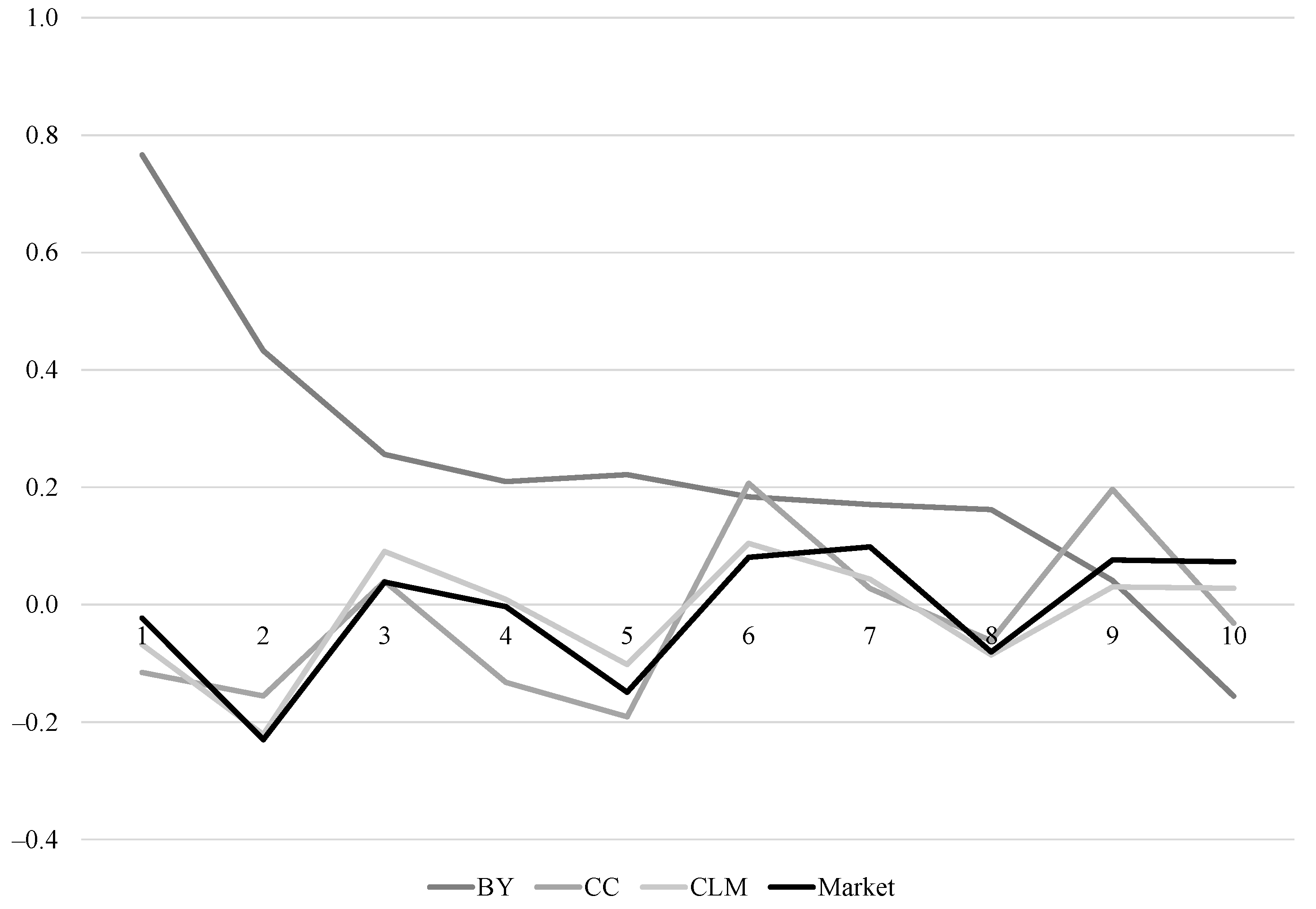
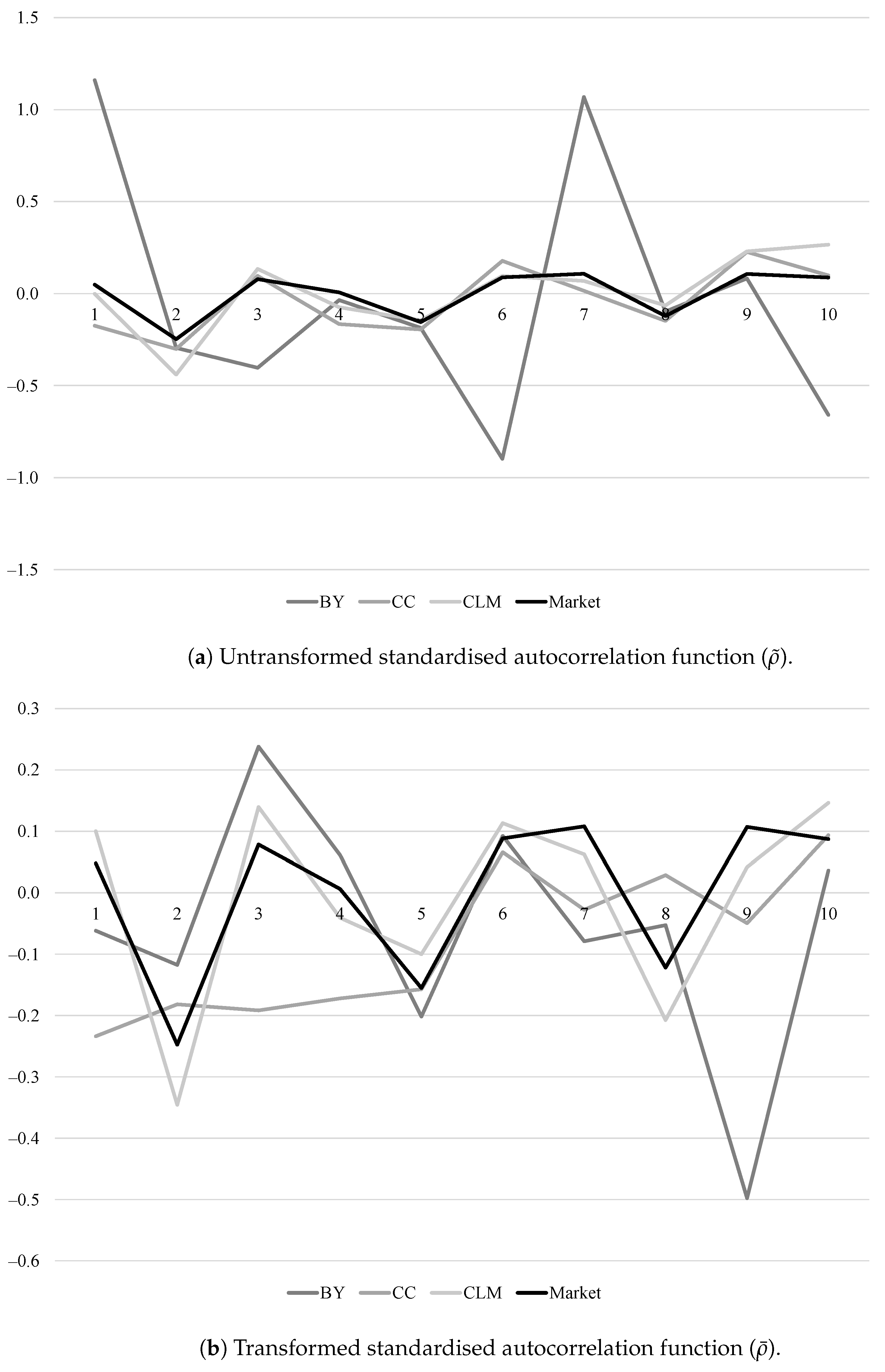
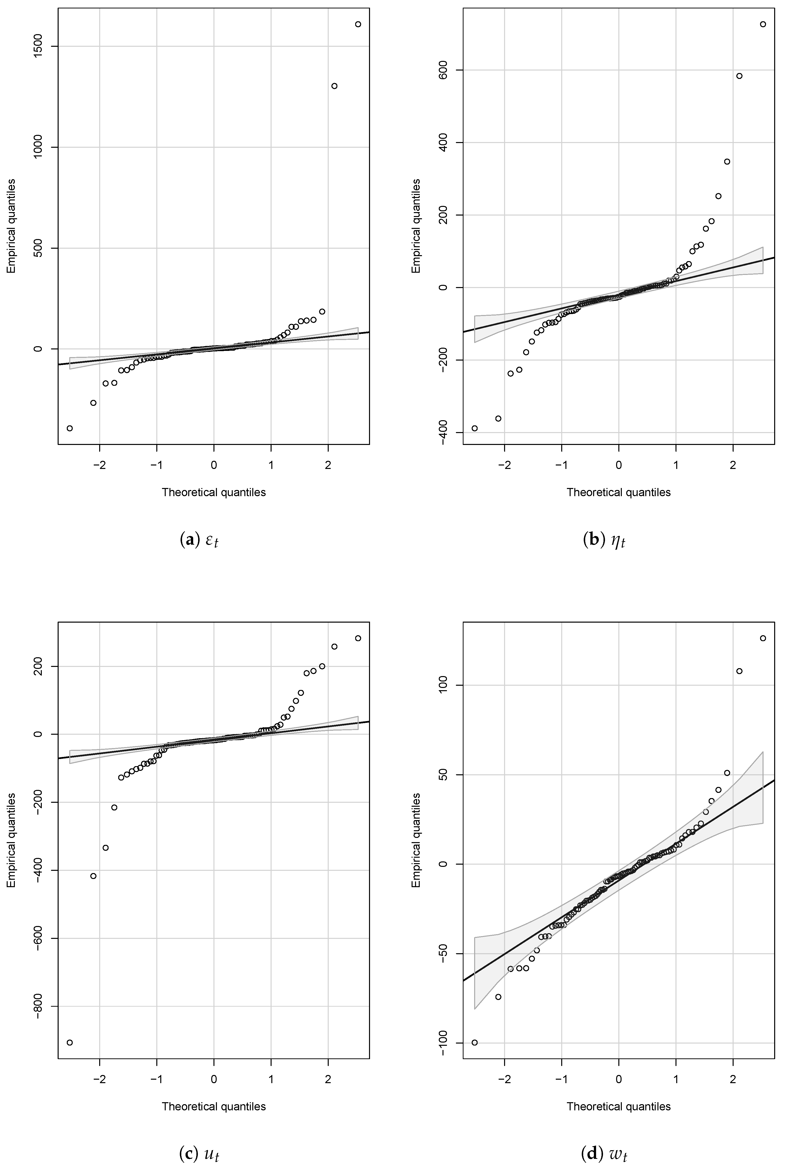
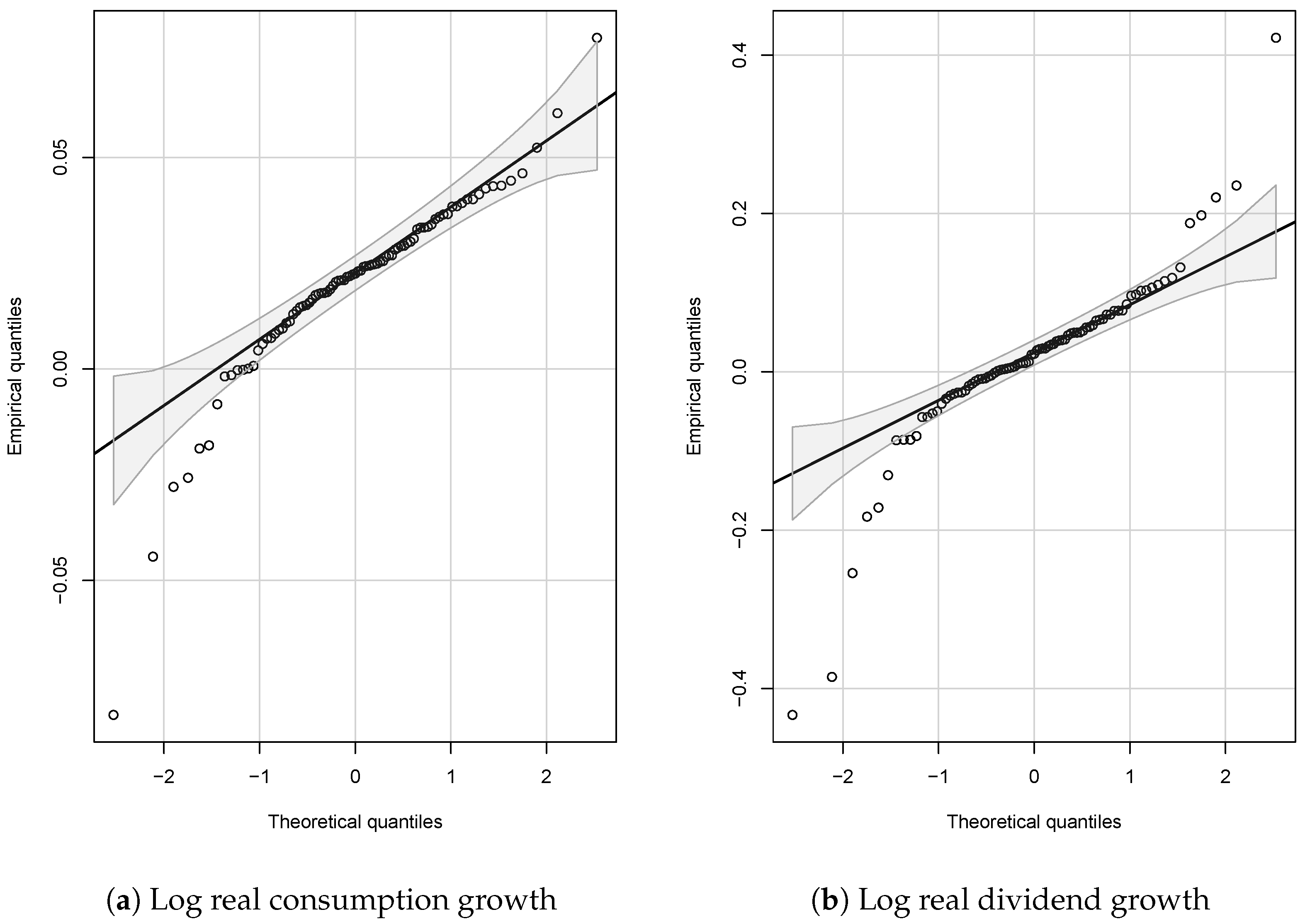
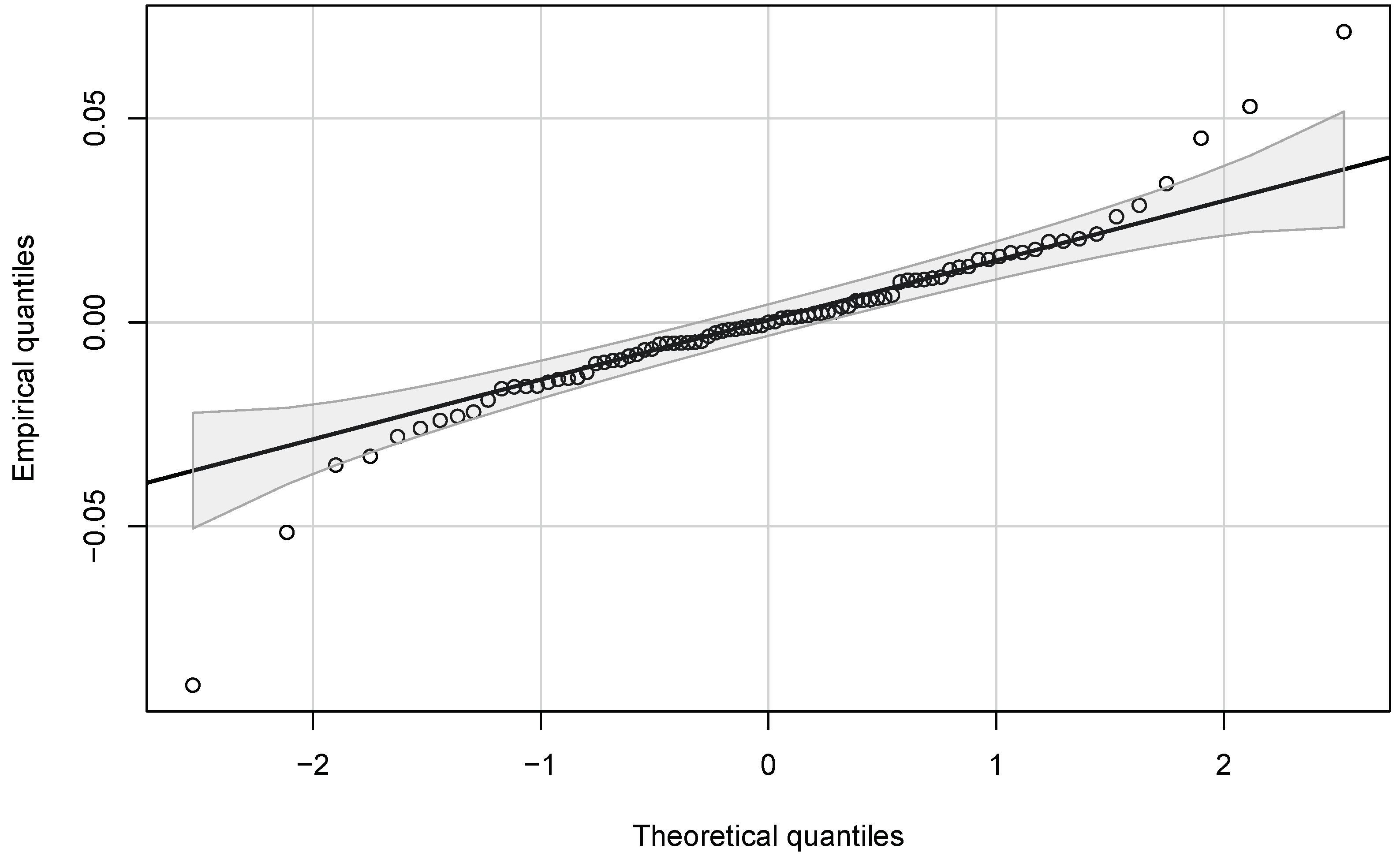
Table 1.
Data summary statistics.
| Mean | Median | Std Dev | ||
|---|---|---|---|---|
| 0.063 | 0.105 | 0.194 | −0.024 | |
| 0.005 | 0.008 | 0.037 | 0.762 | |
| 0.020 | 0.023 | 0.022 | 0.466 | |
| 0.017 | 0.023 | 0.111 | 0.192 | |
| 3.409 | 3.393 | 0.455 | 0.885 |
Descriptive statistics for our key variables at the annual frequency over the period of 1930–2016. denotes the log market return, the quarterly log risk-free rate (the rolled-over 1 month US T-bill), the log consumption growth, the log dividend growth and the log price–dividend ratio. “Std dev” denotes standard deviation and “” denotes estimated first-order serial correlation.
Table 2.
Bansal–Yaron model estimates.
| 0.016 | 0.014 | 4.004 | 5.778 | 0.802 | 0.846 | 0.011 | 0.258 | 0.000 | 0.988 | 2.072 | 7.924 |
| (0.003) | (0.013) | (0.757) | (3.661) | (0.343) | (1.214) | (0.004) | (10.17) | (0.011) | (0.208) | (40.22) | (25.41) |
| 0.000 | 0.274 | 0.000 | 0.115 | 0.020 | 0.486 | 0.009 | 0.980 | 0.997 | 0.000 | 0.959 | 0.755 |
| J-stat | 43.89 | p-value | 0.000 |
Estimates of the Bansal–Yaron model parameters using annual US data, 1930–2016. Point estimates are displayed in the first row, standard errors (in parentheses) in the second and p-values in the third. All p-values are asymptotic.
Table 3.
Properties of .
| Model | Mean | Median | Std Dev | |
|---|---|---|---|---|
| Bansal–Yaron | −0.066 | −0.097 | 0.444 | 0.589 |
| Campbell–Cochrane | 0.007 | −0.012 | 0.210 | −0.115 |
| Cecchetti–Lam–Mark | −0.017 | 0.014 | 0.191 | −0.080 |
Summary statistics for the model-implied ex ante residuals. “Std dev” denotes standard deviation and “” estimated first-order serial correlation. The models are estimated and residuals computed using annual US data over the period of 1930–2016.
Table 4.
Campbell–Cochrane model estimates.
| 0.021 | 0.012 | 0.001 | 0.424 | 0.879 | 0.929 | 0.043 | |
| (0.003) | () | (0.004) | (0.001) | (0.173) | (0.050) | (0.020) | (0.836) |
| 0.000 | 0.007 | 0.003 | 0.056 | 0.017 | 0.000 | 0.000 | 0.959 |
| J-stat | 0.089 | 0.783 | J-stat | 36.24 | |||
| p-value | 0.766 | p-value | 0.000 |
Estimates of the Campbell–Cochrane model parameters using annual US data, 1930–2016. Each panel (set of columns) refers to a separate estimation. The estimates of δ and γ, and the associated p-values, condition on the estimates in the first two panels. Point estimates are displayed in the first row, standard errors (in parentheses) in the second and p-values in the third. All p-values are asymptotic.
Table 5.
Cecchetti–Lam–Mark model estimates.
| (a) Consumption model | |||||
| p | q | ||||
| 0.023 | −0.016 | 0.956 | 0.876 | 0.012 | 0.040 |
| (b) Preference parameters | |||||
| 0.966 | 2.431 | ||||
| (0.290) | (15.38) | ||||
| 0.001 | 0.874 | ||||
| J-stat | 37.18 | ||||
| p-value | 0.000 | ||||
Estimates of the Cecchetti–Lam–Mark model parameters, estimated using annual US data, 1930–2016. Panel (a) presents point estimates only. In panel (b), point estimates are displayed in the first row, standard errors (in parentheses) in the second and p-values in the third. All p-values are asymptotic.
Table 6.
Bansal–Yaron model results.
| (a) Correlogram | |||||||||
| q | 2 | 3 | 4 | 5 | 6 | 7 | 8 | 9 | 10 |
| −0.015 | −0.083 | −0.039 | −0.013 | −0.032 | −0.048 | −0.095 | −0.083 | −0.157 | |
| (Std Err) | (0.054) | (0.080) | (0.101) | (0.118) | (0.133) | (0.147) | (0.159) | (0.171) | (0.182) |
| p-value | 0.783 | 0.303 | 0.702 | 0.914 | 0.808 | 0.745 | 0.551 | 0.628 | 0.390 |
| (b) Quantilogram | |||||||||
| ↓/q→ | 2 | 3 | 4 | 5 | 6 | 7 | 8 | 9 | 10 |
| 0.01 | −0.003 | −0.006 | −0.009 | −0.013 | −0.016 | −0.020 | −0.024 | −0.028 | −0.032 |
| 0.00 | 0.00 | 0.00 | 0.00 | 0.00 | 0.00 | 0.00 | 0.00 | 0.00 | |
| 0.05 | 0.219 | 0.277 | 0.335 | 0.456 | 0.584 | 0.667 | 0.724 | 0.763 | 0.788 |
| 0.81 | 0.38 | 0.31 | 0.27 | 0.23 | 0.23 | 0.21 | 0.19 | 0.14 | |
| 0.1 | 0.145 | 0.245 | 0.367 | 0.471 | 0.542 | 0.609 | 0.664 | 0.695 | 0.735 |
| 0.05 | 0.02 | 0.01 | 0.01 | 0.01 | 0.01 | 0.00 | 0.00 | 0.00 | |
| 0.25 | 0.208 | 0.337 | 0.485 | 0.635 | 0.741 | 0.829 | 0.910 | 0.967 | 1.009 |
| 0.00 | 0.00 | 0.00 | 0.00 | 0.00 | 0.00 | 0.00 | 0.00 | 0.00 | |
| 0.5 | 0.185 | 0.318 | 0.443 | 0.558 | 0.665 | 0.745 | 0.830 | 0.898 | 0.947 |
| 0.00 | 0.00 | 0.00 | 0.00 | 0.00 | 0.00 | 0.00 | 0.00 | 0.00 | |
| 0.75 | 0.224 | 0.412 | 0.562 | 0.707 | 0.817 | 0.902 | 0.972 | 1.030 | 1.084 |
| 0.00 | 0.00 | 0.00 | 0.00 | 0.00 | 0.00 | 0.00 | 0.00 | 0.00 | |
| 0.9 | 0.119 | 0.181 | 0.261 | 0.349 | 0.410 | 0.464 | 0.498 | 0.526 | 0.549 |
| 0.15 | 0.02 | 0.00 | 0.00 | 0.00 | 0.00 | 0.00 | 0.00 | 0.00 | |
| 0.95 | 0.157 | 0.236 | 0.328 | 0.376 | 0.403 | 0.416 | 0.421 | 0.421 | 0.417 |
| 0.63 | 0.30 | 0.14 | 0.08 | 0.04 | 0.03 | 0.02 | 0.01 | 0.01 | |
| 0.99 | 0.195 | 0.255 | 0.284 | 0.300 | 0.310 | 0.316 | 0.320 | 0.323 | 0.324 |
| 0.13 | 0.31 | 0.50 | 0.65 | 0.79 | 0.91 | 1.00 | 0.91 | 0.85 | |
| (c) Hong–Lee tests | |||||||||
| q | 2 | 3 | 4 | 5 | 6 | 7 | 8 | 9 | 10 |
| 1.476 | 1.482 | 1.489 | 1.496 | 1.503 | 1.510 | 1.517 | 1.524 | 1.531 | |
| p-value | 0.140 | 0.138 | 0.136 | 0.135 | 0.133 | 0.131 | 0.129 | 0.127 | 0.126 |
| (d) Mincer–Zarnowitz regression | |||||||||
| Constant | Expected return | MZ F-stat | |||||||
| Coefficient | 0.093 | 0.079 | 145.3 | ||||||
| (Std err) | (0.019) | (0.090) | |||||||
| p-value | 0.000 | 0.386 | 0.000 | ||||||
| (e) Rescaled range | |||||||||
| 1.566 | |||||||||
| p-value | 0.00 | ||||||||
| (f) Linear MIDAS test | |||||||||
| 2.593 | |||||||||
| p-value | 0.273 | ||||||||
| (g) SP MIDAS test | |||||||||
| −0.573 | |||||||||
| p-value | 0.190 | ||||||||
| (h) Maximal predictability | |||||||||
| q | 2 | 3 | 4 | 5 | 6 | 7 | 8 | 9 | 10 |
| 0.100 | 0.044 | 0.462 | 0.002 | 0.038 | 0.043 | 0.125 | 0.028 | 0.000 | |
| 21.68 | 0.122 | −12.29 | −59.18 | −0.725 | −2.738 | 1993 | 67.57 | 1.058 | |
| Wald stat | - | - | 42.19 | 54.06 | 50.13 | 5.156 | - | - | - |
| p-value | - | - | 0.000 | 0.000 | 0.000 | 0.023 | - | - | - |
denotes the estimated transformed weighted correlogram statistic, . Its standard error and asymptotic p-value are given underneath. In Panel (b), the estimated weighted quantilogram is given in larger font for the appropriate combination. Its bootstrapped p-value is given underneath in smaller font. denotes the Hong–Lee generalised spectral statistic. Its asymptotic p-value is given beneath. Panel (d) shows the Mincer–Zarnowitz regression estimates, with the relevant HAC standard errors (in parentheses) and p-values below, along with the HAC F-statistic testing the joint null that the constant is zero and the expected return coefficient is one. denotes the estimated rescaled range. Its bootstrapped p-value is given beneath. denotes the MIDAS Wald statistic, and its asymptotic p-value is given beneath. is the estimated Hsiao et al. (2007) consistent model specification statistic from the semi-parametric MIDAS model. Its bootstrapped p-value is given beneath. Panel (h) reports tests of the null that the market return is no more predictable than implied by Bansal–Yaron model state variables (i.e., ). The Wald statistic and its asymptotic p-value are reported.
Table 7.
Campbell–Cochrane model results.
| (a) Correlogram | |||||||||
| q | 2 | 3 | 4 | 5 | 6 | 7 | 8 | 9 | 10 |
| −0.117 | −0.170 | −0.196 | −0.239 | −0.304 | −0.341 | −0.430 | −0.442 | −0.452 | |
| (Std err) | (0.054) | (0.080) | (0.101) | (0.118) | (0.133) | (0.147) | (0.159) | (0.171) | (0.182) |
| p-value | 0.030 | 0.035 | 0.052 | 0.043 | 0.022 | 0.020 | 0.007 | 0.010 | 0.013 |
| (b) Quantilogram | |||||||||
| ↓/q→ | 2 | 3 | 4 | 5 | 6 | 7 | 8 | 9 | 10 |
| 0.01 | −0.003 | −0.014 | 0.017 | 0.026 | −0.006 | −0.059 | −0.064 | −0.030 | −0.009 |
| 0.06 | 0.61 | 0.57 | 0.78 | 0.69 | 0.70 | 0.89 | 0.77 | 0.06 | |
| 0.05 | −0.006 | −0.028 | −0.012 | −0.020 | −0.080 | −0.120 | −0.088 | 0.024 | −0.018 |
| 0.23 | 0.97 | 0.74 | 0.57 | 0.71 | 0.64 | 0.73 | 0.83 | 0.23 | |
| 0.1 | −0.009 | −0.043 | −0.052 | −0.086 | −0.114 | −0.132 | −0.129 | 0.038 | −0.026 |
| 0.56 | 0.98 | 0.82 | 0.71 | 0.76 | 0.79 | 0.80 | 0.83 | 0.25 | |
| 0.25 | −0.013 | −0.058 | −0.070 | −0.140 | −0.150 | −0.141 | −0.137 | 0.037 | −0.035 |
| 0.70 | 0.96 | 0.84 | 0.69 | 0.93 | 0.98 | 0.97 | 0.95 | 0.25 | |
| 0.5 | −0.016 | −0.073 | −0.101 | −0.183 | −0.179 | −0.157 | −0.163 | 0.029 | −0.044 |
| 0.86 | 0.92 | 0.96 | 0.83 | 0.99 | 0.90 | 0.80 | 0.92 | 0.25 | |
| 0.75 | −0.020 | −0.042 | −0.099 | −0.217 | −0.186 | −0.150 | −0.160 | 0.015 | −0.053 |
| 0.91 | 0.94 | 0.99 | 0.90 | 0.92 | 0.75 | 0.75 | 0.94 | 0.36 | |
| 0.9 | −0.024 | −0.001 | −0.092 | −0.234 | −0.190 | −0.141 | −0.173 | −0.001 | −0.062 |
| 1.00 | 0.94 | 0.96 | 0.97 | 0.88 | 0.66 | 0.70 | 1.00 | 0.38 | |
| 0.95 | −0.028 | 0.029 | −0.098 | −0.230 | −0.201 | −0.143 | −0.197 | −0.020 | −0.071 |
| 0.94 | 0.96 | 0.93 | 0.96 | 0.82 | 0.62 | 0.67 | 0.99 | 0.44 | |
| 0.99 | 0.004 | 0.052 | −0.113 | −0.212 | −0.198 | −0.142 | −0.222 | −0.040 | −0.080 |
| 0.99 | 0.86 | 0.81 | 0.85 | 0.62 | 0.52 | 0.48 | 0.61 | 0.38 | |
| (c) Hong–Lee tests | |||||||||
| q | 2 | 3 | 4 | 5 | 6 | 7 | 8 | 9 | 10 |
| 0.381 | 0.386 | 0.388 | 0.386 | 0.383 | 0.379 | 0.373 | 0.365 | 0.345 | |
| p-value | 0.703 | 0.699 | 0.698 | 0.699 | 0.702 | 0.705 | 0.709 | 0.715 | 0.730 |
| (d) Mincer–Zarnowitz regression | |||||||||
| Constant | Expected return | MZ F-stat | |||||||
| Coefficient | 0.080 | −0.287 | 1.342 | ||||||
| (Std err) | (0.050) | (1.070) | |||||||
| p-value | 0.117 | 0.790 | 0.273 | ||||||
| (e) Rescaled range | |||||||||
| 0.911 | |||||||||
| p-value | 0.28 | ||||||||
| (f) SP MIDAS test | |||||||||
| −0.466 | |||||||||
| p-value | 0.063 | ||||||||
| (g) Maximal predictability | |||||||||
| q | 2 | 3 | 4 | 5 | 6 | 7 | 8 | 9 | 10 |
| 0.057 | 0.022 | 0.012 | 0.029 | 0.035 | 0.039 | 0.020 | 0.002 | ||
| 0.127 | 0.001 | 0.067 | 0.010 | 0.045 | 0.012 | 0.025 | 0.030 | ||
| Wald stat | - | 16.91 | - | 0.185 | 7.920 | - | 4.618 | - | - |
| p-value | - | 0.000 | - | 0.667 | 0.005 | - | 0.032 | - | - |
denotes the estimated transformed weighted correlogram statistic, . Its standard error and asymptotic p-value are given underneath. In Panel (b), the estimated weighted quantilogram is given in larger font for the appropriate combination. Its bootstrapped p-value is given underneath in smaller font. denotes the Hong–Lee generalised spectral statistic. Its asymptotic p-value is given beneath. Panel (d) shows the Mincer–Zarnowitz regression estimates, with the relevant HAC standard errors (in parentheses) and p-values below, along with the HAC F-statistic testing the joint null that the constant is zero and the expected return coefficient is one. denotes the estimated rescaled range. Its bootstrapped p-value is given beneath. is the estimated Hsiao et al. (2007) consistent model specification statistic from the semi-parametric MIDAS model. Its bootstrapped p-value is given beneath. Panel (g) reports tests of the null that the market return is no more predictable than implied by the Campbell–Cochrane model state variables (i.e., ). The Wald statistic and its asymptotic p-value are reported.
Table 8.
Cecchetti–Lam–Mark model results.
| (a) Correlogram | |||||||||
| q | 2 | 3 | 4 | 5 | 6 | 7 | 8 | 9 | 10 |
| 0.043 | −0.087 | −0.201 | −0.275 | −0.342 | −0.361 | −0.428 | −0.455 | −0.526 | |
| (Std err) | (0.054) | (0.080) | (0.101) | (0.118) | (0.133) | (0.147) | (0.159) | (0.171) | (0.182) |
| p-value | 0.425 | 0.278 | 0.047 | 0.020 | 0.010 | 0.014 | 0.007 | 0.008 | 0.004 |
| (b) Quantilogram | |||||||||
| / | 2 | 3 | 4 | 5 | 6 | 7 | 8 | 9 | 10 |
| 0.01 | −0.009 | 0.018 | 0.080 | 0.165 | 0.262 | 0.359 | 0.448 | 0.526 | 0.587 |
| 0.39 | 0.77 | 0.98 | 0.78 | 0.74 | 0.67 | 0.67 | 0.66 | 0.71 | |
| 0.05 | −0.006 | −0.017 | −0.036 | −0.053 | −0.070 | −0.090 | −0.104 | −0.116 | −0.126 |
| 0.72 | 0.78 | 0.72 | 0.66 | 0.61 | 0.57 | 0.57 | 0.58 | 0.47 | |
| 0.1 | −0.004 | −0.014 | −0.030 | −0.047 | −0.063 | −0.084 | −0.099 | −0.116 | −0.132 |
| 0.76 | 0.67 | 0.62 | 0.60 | 0.53 | 0.51 | 0.47 | 0.45 | 0.39 | |
| 0.25 | 0.015 | 0.004 | −0.005 | −0.016 | −0.026 | −0.039 | −0.053 | −0.072 | −0.094 |
| 0.86 | 0.75 | 0.70 | 0.67 | 0.60 | 0.57 | 0.53 | 0.48 | 0.42 | |
| 0.5 | 0.031 | 0.028 | 0.032 | 0.035 | 0.029 | 0.016 | 0.000 | −0.021 | −0.045 |
| 0.99 | 0.95 | 0.87 | 0.85 | 0.78 | 0.73 | 0.72 | 0.70 | 0.59 | |
| 0.75 | 0.089 | 0.115 | 0.147 | 0.170 | 0.179 | 0.178 | 0.167 | 0.145 | 0.120 |
| 0.97 | 0.87 | 0.87 | 0.85 | 0.81 | 0.77 | 0.77 | 0.73 | 0.66 | |
| 0.9 | 0.069 | 0.081 | 0.082 | 0.082 | 0.076 | 0.063 | 0.049 | 0.030 | 0.009 |
| 0.98 | 0.92 | 0.88 | 0.86 | 0.86 | 0.80 | 0.76 | 0.73 | 0.60 | |
| 0.95 | 0.009 | 0.009 | −0.004 | −0.018 | −0.035 | −0.055 | −0.075 | −0.098 | −0.119 |
| 0.91 | 0.84 | 0.75 | 0.74 | 0.69 | 0.67 | 0.64 | 0.63 | 0.49 | |
| 0.99 | −0.009 | −0.025 | −0.051 | −0.100 | −0.170 | −0.259 | −0.367 | −0.495 | −0.650 |
| 0.41 | 0.45 | 0.47 | 0.49 | 0.52 | 0.51 | 0.52 | 0.53 | 0.48 | |
| (c) Hong–Lee tests | |||||||||
| q | 2 | 3 | 4 | 5 | 6 | 7 | 8 | 9 | 10 |
| 0.884 | 0.897 | 0.904 | 0.907 | 0.907 | 0.903 | 0.894 | 0.882 | 0.867 | |
| p-value | 0.377 | 0.370 | 0.366 | 0.364 | 0.364 | 0.367 | 0.371 | 0.378 | 0.386 |
| (d) Mincer–Zarnowitz regression | |||||||||
| Constant | Expected return | MZ F-stat | |||||||
| Coefficient | 0.079 | −0.154 | 0.763 | ||||||
| (Std err) | (0.072) | (0.940) | |||||||
| p-value | 0.278 | 0.871 | 0.473 | ||||||
| (e) Rescaled range | |||||||||
| 0.698 | |||||||||
| p-value | 0.02 | ||||||||
| (f) SP MIDAS test | |||||||||
| −0.725 | |||||||||
| p-value | 0.602 | ||||||||
| (g) Maximal predictability | |||||||||
| q | 2 | 3 | 4 | 5 | 6 | 7 | 8 | 9 | 10 |
| 0.057 | 0.022 | 0.012 | 0.000 | 0.029 | 0.035 | 0.039 | 0.020 | 0.002 | |
| 0.006 | 0.026 | 0.033 | 0.160 | 0.194 | 0.026 | 0.050 | 0.362 | 0.346 | |
| Wald stat | 134.1 | - | - | - | - | 0.189 | - | - | - |
| p-value | 0.000 | - | - | - | - | 0.664 | - | - | - |
denotes the estimated transformed weighted correlogram statistic, . Its standard error and asymptotic p-value are given underneath. In Panel (b), the estimated weighted quantilogram is given in larger font for the appropriate combination. Its bootstrapped p-value is given underneath in smaller font. denotes the Hong–Lee generalised spectral statistic. Its asymptotic p-value is given beneath. Panel (d) shows the Mincer–Zarnowitz regression estimates, with the relevant HAC standard errors (in parentheses) and p-values below, along with the HAC F-statistic testing the joint null that the constant is zero and the expected return coefficient is one. denotes the estimated rescaled range. Its bootstrapped p-value is given beneath. is the estimated Hsiao et al. (2007) consistent model specification statistic from the semi-parametric MIDAS model. Its bootstrapped p-value is given beneath. Panel (g) reports tests of the null that the market return is no more predictable than implied by the Cecchetti–Lam–Mark model state variables (i.e., ). The Wald statistic and its asymptotic p-value are reported.
Table 9.
Properties of —Identity matrix.
| Model | Mean | Median | Std Dev | |
|---|---|---|---|---|
| Campbell–Cochrane | −0.466 | −0.397 | 0.289 | 0.455 |
| Cecchetti–Lam–Mark | −0.038 | −0.040 | 0.191 | −0.088 |
Summary statistics for the model-implied ex ante residuals. “Std dev” denotes standard deviation and “” estimated first-order serial correlation. The models are estimated and residuals computed using annual US data over the period of 1930–2016.
Table 10.
Cecchetti–Lam–Mark model results—Identity matrix.
| (a) Correlogram | |||||||||
| q | 2 | 3 | 4 | 5 | 6 | 7 | 8 | 9 | 10 |
| 0.026 | −0.122 | −0.190 | −0.260 | −0.300 | −0.311 | −0.351 | −0.381 | −0.390 | |
| (Std err) | (0.054) | (0.080) | (0.101) | (0.118) | (0.133) | (0.147) | (0.159) | (0.171) | (0.182) |
| p-value | 0.633 | 0.129 | 0.059 | 0.028 | 0.025 | 0.034 | 0.028 | 0.026 | 0.032 |
| (b) Quantilogram | |||||||||
| / | 2 | 3 | 4 | 5 | 6 | 7 | 8 | 9 | 10 |
| 0.01 | −0.003 | −0.006 | −0.009 | −0.013 | −0.016 | −0.020 | −0.024 | −0.028 | 0.004 |
| 0.40 | 0.75 | 0.99 | 0.83 | 0.80 | 0.70 | 0.70 | 0.69 | 0.76 | |
| 0.05 | −0.014 | −0.028 | −0.043 | −0.058 | −0.073 | −0.042 | −0.022 | −0.007 | 0.004 |
| 0.74 | 0.80 | 0.78 | 0.70 | 0.69 | 0.65 | 0.61 | 0.59 | 0.47 | |
| 0.1 | 0.017 | 0.011 | −0.018 | −0.003 | 0.012 | 0.047 | 0.060 | 0.067 | 0.063 |
| 0.68 | 0.66 | 0.54 | 0.55 | 0.51 | 0.49 | 0.46 | 0.45 | 0.38 | |
| 0.25 | 0.026 | −0.053 | −0.111 | −0.111 | −0.136 | −0.157 | −0.154 | −0.146 | −0.147 |
| 0.74 | 0.70 | 0.60 | 0.54 | 0.53 | 0.49 | 0.47 | 0.41 | 0.37 | |
| 0.5 | −0.030 | −0.136 | −0.162 | −0.192 | −0.260 | −0.301 | −0.318 | −0.337 | −0.350 |
| 0.70 | 0.66 | 0.60 | 0.48 | 0.46 | 0.44 | 0.35 | 0.33 | 0.25 | |
| 0.75 | −0.059 | −0.100 | −0.140 | −0.134 | −0.140 | −0.119 | −0.126 | −0.130 | −0.137 |
| 0.64 | 0.62 | 0.56 | 0.50 | 0.46 | 0.47 | 0.44 | 0.39 | 0.30 | |
| 0.9 | −0.003 | 0.034 | 0.084 | 0.139 | 0.199 | 0.227 | 0.251 | 0.275 | 0.310 |
| 0.76 | 0.79 | 0.65 | 0.57 | 0.49 | 0.44 | 0.42 | 0.36 | 0.26 | |
| 0.95 | −0.030 | 0.024 | 0.070 | 0.137 | 0.197 | 0.234 | 0.258 | 0.272 | 0.280 |
| 0.79 | 0.68 | 0.58 | 0.56 | 0.49 | 0.45 | 0.40 | 0.38 | 0.33 | |
| 0.99 | −0.009 | −0.018 | −0.024 | −0.030 | −0.036 | −0.041 | −0.047 | −0.052 | −0.057 |
| 0.31 | 0.38 | 0.40 | 0.35 | 0.37 | 0.39 | 0.38 | 0.40 | 0.34 | |
| (c) Hong–Lee tests | |||||||||
| q | 2 | 3 | 4 | 5 | 6 | 7 | 8 | 9 | 10 |
| 0.782 | 0.795 | 0.801 | 0.803 | 0.803 | 0.800 | 0.793 | 0.783 | 0.770 | |
| p-value | 0.434 | 0.427 | 0.423 | 0.422 | 0.422 | 0.424 | 0.428 | 0.434 | 0.441 |
| (d) Mincer–Zarnowitz regression | |||||||||
| Constant | Expected return | MZ F-stat | |||||||
| Coefficient | 0.132 | −0.459 | 4.039 | ||||||
| (Std err) | (0.231) | (1.665) | |||||||
| p-value | 0.571 | 0.784 | 0.025 | ||||||
| (e) Rescaled range | |||||||||
| 0.694 | |||||||||
| p-value | 0.01 | ||||||||
denotes the estimated transformed weighted correlogram statistic, . Its standard error and asymptotic p-value are given underneath. In Panel (b), the estimated weighted quantilogram is given in larger font for the appropriate combination. Its bootstrapped p-value is given underneath in smaller font. denotes the Hong–Lee generalised spectral statistic. Its asymptotic p-value is given beneath. Panel (d) shows the Mincer–Zarnowitz regression estimates, with the relevant HAC standard errors (in parentheses) and p-values below, along with the HAC F-statistic testing the joint null that the constant is zero and the expected return coefficient is one. In Panel (e), denotes the estimated rescaled range. Its bootstrapped p-value is given beneath.
Table 11.
Properties of —Industry portfolios.
| Model | Mean | Median | Std Dev | |
|---|---|---|---|---|
| Optimal weight matrix | ||||
| Bansal–Yaron | - | - | - | - |
| Campbell–Cochrane | −0.250 | −0.279 | 0.232 | −0.045 |
| Cecchetti–Lam–Mark | −0.185 | −0.158 | 0.194 | −0.041 |
| Identity weight matrix | ||||
| Bansal–Yaron | −0.685 | −0.715 | 0.426 | 0.564 |
| Campbell–Cochrane | −0.115 | −0.130 | 0.257 | −0.126 |
| Cecchetti–Lam–Mark | −0.242 | −0.098 | 0.376 | 0.567 |
Summary statistics for the model-implied ex ante residuals. “Std dev” denotes standard deviation and “” estimated first-order serial correlation. The models are estimated and residuals computed using annual US data over the period of 1930–2016.
Table 12.
Campbell–Cochrane model results—Industry portfolios and identity matrix.
| (a) Correlogram | |||||||||
| q | 2 | 3 | 4 | 5 | 6 | 7 | 8 | 9 | 10 |
| −0.142 | −0.220 | 0.028 | −0.040 | 0.039 | −0.149 | 0.179 | 0.303 | 0.318 | |
| (Std err) | (0.054) | (0.080) | (0.101) | (0.118) | (0.133) | (0.147) | (0.159) | (0.171) | (0.182) |
| p-value | 0.009 | 0.006 | 0.782 | 0.733 | 0.768 | 0.310 | 0.261 | 0.076 | 0.080 |
| (b) Quantilogram | |||||||||
| / | 2 | 3 | 4 | 5 | 6 | 7 | 8 | 9 | 10 |
| 0.01 | −0.003 | −0.006 | −0.009 | −0.009 | −0.006 | −0.003 | 0.001 | 0.006 | 0.010 |
| 0.00 | 0.00 | 0.00 | 0.00 | 0.00 | 0.00 | 0.00 | 0.00 | 0.00 | |
| 0.05 | −0.014 | −0.028 | 0.078 | 0.138 | 0.176 | 0.224 | 0.259 | 0.285 | 0.305 |
| 0.00 | 0.00 | 0.00 | 0.00 | 0.00 | 0.00 | 0.00 | 0.00 | 0.00 | |
| 0.1 | 0.017 | 0.011 | 0.083 | 0.135 | 0.155 | 0.194 | 0.246 | 0.278 | 0.311 |
| 0.00 | 0.00 | 0.00 | 0.00 | 0.00 | 0.00 | 0.00 | 0.00 | 0.00 | |
| 0.25 | −0.022 | −0.037 | −0.027 | −0.058 | −0.082 | −0.069 | −0.065 | −0.057 | −0.064 |
| 0.00 | 0.00 | 0.00 | 0.00 | 0.00 | 0.00 | 0.00 | 0.00 | 0.00 | |
| 0.5 | −0.065 | −0.111 | −0.113 | −0.158 | −0.195 | −0.210 | −0.207 | −0.208 | −0.212 |
| 0.00 | 0.00 | 0.00 | 0.00 | 0.00 | 0.00 | 0.00 | 0.00 | 0.00 | |
| 0.75 | −0.029 | −0.090 | −0.121 | −0.151 | −0.154 | −0.133 | −0.113 | −0.115 | −0.116 |
| 0.00 | 0.00 | 0.00 | 0.00 | 0.00 | 0.00 | 0.00 | 0.00 | 0.00 | |
| 0.9 | −0.034 | −0.047 | −0.083 | −0.099 | −0.130 | −0.148 | −0.160 | −0.183 | −0.199 |
| 0.00 | 0.00 | 0.00 | 0.00 | 0.00 | 0.00 | 0.00 | 0.00 | 0.00 | |
| 0.95 | −0.030 | −0.059 | −0.086 | −0.080 | −0.083 | −0.092 | −0.106 | −0.121 | −0.139 |
| 0.02 | 0.00 | 0.00 | 0.00 | 0.00 | 0.00 | 0.00 | 0.00 | 0.00 | |
| 0.99 | −0.009 | −0.018 | −0.026 | −0.041 | −0.059 | −0.079 | −0.099 | −0.121 | −0.144 |
| 0.62 | 0.47 | 0.47 | 0.47 | 0.44 | 0.42 | 0.42 | 0.42 | 0.42 | |
| (c) Hong–Lee tests | |||||||||
| q | 2 | 3 | 4 | 5 | 6 | 7 | 8 | 9 | 10 |
| 0.491 | 0.511 | 0.527 | 0.539 | 0.548 | 0.556 | 0.562 | 0.568 | 0.575 | |
| p-value | 0.624 | 0.609 | 0.598 | 0.590 | 0.584 | 0.579 | 0.574 | 0.570 | 0.566 |
| (d) Mincer–Zarnowitz regression | |||||||||
| Constant | Expected return | MZ F-stat | |||||||
| Coefficient | 0.412 | −0.022 | 182,144 | ||||||
| (Std err) | (0.528) | (0.035) | |||||||
| p-value | 0.439 | 0.522 | 0.000 | ||||||
| (e) Rescaled range | |||||||||
| 0.946 | |||||||||
| p-value | 0.00 | ||||||||
denotes the estimated transformed weighted correlogram statistic, . Its standard error and asymptotic p-value are given underneath. In Panel (b), the estimated weighted quantilogram is given in larger font for the appropriate combination. Its bootstrapped p-value is given underneath in a smaller font. denotes the Hong–Lee generalised spectral statistic. Its asymptotic p-value is given beneath. Panel (d) shows the Mincer–Zarnowitz regression estimates, with the relevant HAC standard errors (in parentheses) and p-values below, along with the HAC F-statistic testing the joint null that the constant is zero and the expected return coefficient is one. In Panel (e), denotes the estimated rescaled range. Its bootstrapped p-value is given beneath.
Table 13.
Quarterly data summary statistics.
| Mean | Median | Std Dev | ||
|---|---|---|---|---|
| 0.018 | 0.029 | 0.081 | 0.077 | |
| 0.002 | 0.003 | 0.007 | 0.745 | |
| 0.005 | 0.006 | 0.005 | 0.279 | |
| 0.007 | 0.001 | 0.148 | 0.584 | |
| 4.871 | 4.851 | 0.426 | 0.937 |
Descriptive statistics for our key variables at the quarterly frequency over the period of 1947Q1–2017Q1. denotes the log market return, the quarterly log risk-free rate (the rolled-over 1 month US T-bill), the log consumption growth, the log dividend growth and the log price-dividend ratio. “Std dev” denotes standard deviation and “” first-order serial correlation.
Table 14.
Properties of —Quarterly.
| Model | Mean | Median | Std Dev | |
|---|---|---|---|---|
| Optimal weight matrix | ||||
| Bansal–Yaron | - | - | - | - |
| Campbell–Cochrane | −0.351 | −0.341 | 0.091 | 0.264 |
| Cecchetti–Lam–Mark | −0.389 | −0.886 | 0.726 | 0.871 |
| Identity weight matrix | ||||
| Bansal–Yaron | −9.166 | −9.172 | 0.231 | 0.791 |
| Campbell–Cochrane | −0.203 | −0.186 | 0.094 | 0.318 |
| Cecchetti–Lam–Mark | −0.008 | 0.003 | 0.081 | 0.074 |
Summary statistics for the model-implied ex ante residuals. “Std dev” denotes standard deviation and “” first-order serial correlation. The models are estimated and residuals computed using quarterly US data over the period of 1947Q1–2017Q1.
Table 15.
Cecchetti–Lam–Mark model—quarterly results with identity weight matrix.
| (a) Correlogram | |||||||||
| q | 8 | 12 | 16 | 20 | 24 | 28 | 32 | 36 | 40 |
| −0.029 | −0.095 | −0.068 | −0.007 | −0.017 | −0.073 | −0.038 | −0.040 | −0.055 | |
| (Std err) | (0.089) | (0.112) | (0.132) | (0.149) | (0.164) | (0.178) | (0.191) | (0.203) | (0.215) |
| p-value | 0.739 | 0.396 | 0.607 | 0.965 | 0.916 | 0.682 | 0.840 | 0.843 | 0.796 |
| (b) Quantilogram | |||||||||
| / | 8 | 12 | 16 | 20 | 24 | 28 | 32 | 36 | 40 |
| 0.01 | 0.007 | 0.003 | −0.003 | −0.008 | −0.014 | −0.020 | −0.025 | −0.030 | −0.036 |
| 0.57 | 0.78 | 0.85 | 0.95 | 0.78 | 0.66 | 0.48 | 0.39 | 0.35 | |
| 0.05 | 0.044 | 0.054 | 0.054 | 0.049 | 0.038 | 0.024 | 0.013 | 0.006 | 0.000 |
| 0.37 | 0.37 | 0.35 | 0.37 | 0.38 | 0.33 | 0.30 | 0.29 | 0.27 | |
| 0.1 | 0.054 | 0.061 | 0.059 | 0.054 | 0.041 | 0.023 | 0.010 | 0.001 | −0.006 |
| 0.46 | 0.40 | 0.33 | 0.33 | 0.36 | 0.36 | 0.35 | 0.35 | 0.32 | |
| 0.25 | 0.043 | 0.048 | 0.045 | 0.043 | 0.035 | 0.018 | 0.003 | −0.006 | −0.014 |
| 0.42 | 0.41 | 0.41 | 0.39 | 0.36 | 0.32 | 0.34 | 0.36 | 0.33 | |
| 0.5 | 0.008 | 0.009 | 0.005 | 0.001 | −0.004 | −0.008 | −0.014 | −0.020 | −0.025 |
| 0.62 | 0.56 | 0.59 | 0.60 | 0.51 | 0.48 | 0.45 | 0.41 | 0.38 | |
| 0.75 | 0.033 | 0.034 | 0.032 | 0.026 | 0.014 | −0.003 | −0.019 | −0.029 | −0.036 |
| 0.49 | 0.46 | 0.41 | 0.39 | 0.41 | 0.43 | 0.40 | 0.37 | 0.30 | |
| 0.9 | 0.042 | 0.041 | 0.034 | 0.024 | 0.009 | −0.011 | −0.028 | −0.041 | −0.052 |
| 0.43 | 0.45 | 0.44 | 0.46 | 0.53 | 0.53 | 0.55 | 0.49 | 0.43 | |
| 0.95 | 0.045 | 0.049 | 0.044 | 0.034 | 0.020 | 0.004 | −0.009 | −0.018 | −0.027 |
| 0.43 | 0.36 | 0.38 | 0.37 | 0.37 | 0.39 | 0.41 | 0.37 | 0.33 | |
| 0.99 | 0.007 | 0.007 | 0.004 | 0.000 | −0.008 | −0.018 | −0.025 | −0.030 | −0.035 |
| 0.77 | 0.99 | 0.90 | 0.73 | 0.66 | 0.62 | 0.53 | 0.46 | 0.39 | |
| (c) Hong–Lee tests | |||||||||
| q | 8 | 12 | 16 | 20 | 24 | 28 | 32 | 36 | 40 |
| 0.002 | −0.211 | −0.367 | −0.468 | −0.542 | −0.603 | −0.682 | −0.731 | −0.769 | |
| p-value | 0.998 | 0.833 | 0.714 | 0.640 | 0.588 | 0.547 | 0.495 | 0.465 | 0.442 |
| (d) Mincer–Zarnowitz regression | |||||||||
| Constant | Expected return | MZ F-stat | |||||||
| Coefficient | 0.004 | 0.055 | 1082 | ||||||
| (Std err) | (0.018) | (0.049) | |||||||
| p-value | 0.837 | 0.269 | 0.000 | ||||||
| (e) Rescaled range | |||||||||
| 1.076 | |||||||||
| p-value | 0.87 | ||||||||
| (f) SP MIDAS test | |||||||||
| −0.725 | |||||||||
| p-value | 0.602 | ||||||||
| (g) Maximal predictability | |||||||||
| q | 8 | 12 | 16 | 20 | 24 | 28 | 32 | 36 | 40 |
| 0.367 | 0.011 | 0.105 | 0.005 | 0.001 | 0.099 | 0.012 | 0.023 | 0.072 | |
| 1.298 | 0.347 | 0.411 | 3.858 | 0.499 | 3.071 | 3.196 | 0.861 | ||
| Wald stat | - | - | - | - | 10.95 | - | - | - | - |
| p-value | - | - | - | - | 0.001 | - | - | - | - |
denotes the estimated transformed weighted correlogram statistic, . Its standard error and asymptotic p-value are given underneath. In Panel (b), the estimated weighted quantilogram is given in larger font for the appropriate combination. Its bootstrapped p-value is given underneath in a smaller font. denotes the Hong–Lee generalised spectral statistic. Its asymptotic p-value is given beneath. Panel (d) shows the Mincer–Zarnowitz regression estimates, with the relevant HAC standard errors (in parentheses) and p-values below, along with the HAC F-statistic testing the joint null that the constant is zero and the expected return coefficient is one. denotes the estimated rescaled range. Its bootstrapped p-value is given beneath. is the estimated Hsiao et al. (2007) consistent model specification statistic from the semi-parametric MIDAS model. Its bootstrapped p-value is given beneath. Panel (e) reports tests of the null that the market return is no more predictable than implied by the Cecchetti–Lam–Mark model state variables (i.e., ). The Wald statistic and its asymptotic p-value are reported.
Table 16.
Cecchetti–Lam–Mark model quarterly sub-sample results using identity weight matrix.
| (a) Quantilogram—sub-sample 1: 1947Q1–1982Q1 | |||||||||
| / | 8 | 12 | 16 | 20 | 24 | 28 | 32 | 36 | 40 |
| 0.01 | 0.050 | 0.076 | 0.100 | 0.122 | 0.142 | 0.163 | 0.193 | 0.337 | 0.589 |
| 0.02 | 0.02 | 0.02 | 0.06 | 0.07 | 0.09 | 0.09 | 0.65 | 0.62 | |
| 0.05 | 0.092 | 0.093 | 0.075 | 0.076 | 0.065 | 0.042 | 0.010 | −0.009 | −0.036 |
| 0.82 | 0.97 | 0.86 | 0.75 | 0.62 | 0.48 | 0.33 | 0.24 | 0.19 | |
| 0.1 | 0.008 | −0.002 | −0.017 | 0.002 | 0.004 | −0.006 | −0.012 | −0.007 | −0.018 |
| 0.52 | 0.41 | 0.40 | 0.49 | 0.45 | 0.42 | 0.35 | 0.35 | 0.29 | |
| 0.25 | −0.095 | −0.147 | −0.181 | −0.189 | −0.198 | −0.212 | −0.226 | −0.239 | −0.244 |
| 0.06 | 0.04 | 0.03 | 0.03 | 0.03 | 0.03 | 0.02 | 0.02 | 0.01 | |
| 0.5 | −0.052 | −0.133 | −0.191 | −0.207 | −0.200 | −0.203 | −0.221 | −0.236 | −0.232 |
| 0.30 | 0.10 | 0.07 | 0.05 | 0.04 | 0.04 | 0.03 | 0.02 | 0.02 | |
| 0.75 | 0.036 | −0.049 | −0.111 | −0.136 | −0.161 | −0.195 | −0.227 | −0.234 | −0.225 |
| 0.84 | 0.26 | 0.10 | 0.07 | 0.04 | 0.03 | 0.01 | 0.01 | 0.01 | |
| 0.9 | 0.063 | 0.060 | 0.043 | 0.013 | −0.039 | −0.095 | −0.140 | −0.167 | −0.186 |
| 0.97 | 0.75 | 0.59 | 0.38 | 0.23 | 0.16 | 0.11 | 0.09 | 0.08 | |
| 0.95 | 0.008 | 0.011 | −0.002 | −0.025 | −0.066 | −0.107 | −0.142 | −0.166 | −0.183 |
| 0.57 | 0.49 | 0.41 | 0.33 | 0.22 | 0.19 | 0.17 | 0.12 | 0.09 | |
| 0.99 | −0.029 | −0.046 | −0.059 | −0.073 | −0.091 | −0.108 | −0.128 | −0.153 | −0.184 |
| 0.16 | 0.17 | 0.17 | 0.18 | 0.17 | 0.07 | 0.01 | 0.00 | 0.00 | |
| (b) Hong–Lee tests—sub-sample 2: 1982Q2–2017Q1 | |||||||||
| q | 8 | 12 | 16 | 20 | 24 | 28 | 32 | 36 | 40 |
| 20.29 | 19.83 | 19.52 | 19.30 | 19.08 | 18.78 | 18.46 | 18.15 | 17.87 | |
| p-value | 0.000 | 0.000 | 0.000 | 0.000 | 0.000 | 0.000 | 0.000 | 0.000 | 0.000 |
| (c) Correlogram—sub-sample 2: 1982Q2–2017Q1, accounting for look-ahead bias | |||||||||
| q | 8 | 12 | 16 | 20 | 24 | 28 | 32 | 36 | 40 |
| −3.548 | −11.02 | −26.13 | −35.71 | 196.3 | −39.16 | −38.37 | −13.32 | 21.03 | |
| (Std err) | 0.251 | 0.318 | 0.373 | 0.422 | 0.465 | 0.504 | 0.541 | 0.575 | 0.608 |
| p-value | 0.000 | 0.000 | 0.000 | 0.000 | 0.000 | 0.000 | 0.000 | 0.000 | 0.000 |
| (d) Maximal predictability | |||||||||
| q | 8 | 12 | 16 | 20 | 24 | 28 | 32 | 36 | 40 |
| Sub-sample 1: 1947Q1–1982Q1 | |||||||||
| 0.072 | 0.072 | 0.137 | 0.228 | 0.106 | 0.153 | 0.276 | 0.630 | 0.416 | |
| 0.467 | 0.107 | 1.658 | 0.666 | 0.009 | 0.044 | 0.136 | 14.81 | 2.064 | |
| Wald stat | - | - | - | - | 494.3 | 806.1 | 553.0 | - | - |
| p-value | - | - | - | - | 0.000 | 0.000 | 0.000 | - | - |
| Sub-sample 2: 1982Q2–2017Q1 | |||||||||
| 0.023 | 0.156 | 0.262 | 0.161 | 0.071 | 0.076 | 0.546 | 0.792 | 0.519 | |
| 0.084 | 0.126 | 0.002 | 0.010 | 0.409 | 0.009 | 17.462 | 2.665 | 0.204 | |
| Wald stat | - | 0.771 | 442.1 | 167.2 | - | 924.5 | - | - | 13078 |
| p-value | - | 0.380 | 0.000 | 0.000 | - | 0.000 | - | - | 0.000 |
Panel (a) reports the quantilogram tests of the MDS null for the Cecchetti–Lam–Mark model residuals estimated with the identity weight matrix over the first sub-sample, 1947Q1–1982Q1. The estimated weighted quantilogram is given in larger font for the appropriate combination. Its bootstrapped p-value is given underneath in a smaller font. Panel (b) offers the Hong–Lee tests for the residuals from second sub-sample 1982Q2–2017Q1. denotes the Hong–Lee generalised spectral statistic. Its asymptotic p-value is given beneath. Panel (c) reports the weighted correlogram tests for the second sub-sample where estimation uses the identity weight matrix but also accounts for possible look-ahead bias. denotes the estimated transformed weighted correlogram statistic, . Its standard error and asymptotic p-value are given underneath. Panel (d) reports tests of the null that the market return is no more predictable than implied by the Cecchetti–Lam–Mark model state variables (i.e., ) in each of the two sub-samples. The Wald statistic and its asymptotic p-value are reported.
Table 17.
Quarterly semi-parametric MIDAS results.
| Model | p-Value | |
|---|---|---|
| Bansal–Yaron | 1.471 | 0.048 |
| Campbell–Cochrane | ||
| Optimal weight matrix | 0.559 | 0.018 |
| Identity weight matrix | 0.851 | 0.018 |
is the estimated Hsiao et al. (2007) consistent model specification statistic from the semi-parametric MIDAS regression for the asset pricing model and estimation method specified. Its bootstrapped p-value is given in the final column. The Bansal–Yaron model is estimated using the identity weight matrix. Both models are estimated using quarterly data over the period of 1947Q1–2017Q1.
Table 18.
Quarterly maximal predictability results.
| q | 8 | 12 | 16 | 20 | 24 | 28 | 32 | 36 | 40 |
|---|---|---|---|---|---|---|---|---|---|
| Bansal–Yaron model | |||||||||
| 0.057 | 0.018 | 0.069 | 0.025 | 0.012 | 0.119 | 0.011 | 0.159 | ||
| −0.217 | −11.357 | 5.508 | −3.740 | −0.282 | 0.303 | −10.089 | −6.736 | 6.579 | |
| Wald stat | 216,041 | 148,018 | - | 267,587 | 416,715 | - | 593,143 | 1,307,207 | - |
| p-value | 0.000 | 0.000 | - | 0.000 | 0.000 | - | 0.000 | 0.000 | - |
| Campbell–Cochrane model—optimal weight matrix | |||||||||
| 0.029 | 0.041 | 0.059 | 0.001 | 0.005 | 0.006 | 0.082 | |||
| 0.003 | 0.018 | 0.421 | 0.039 | 0.006 | 0.556 | 0.352 | 1.505 | 0.689 | |
| Wald stat | 462.1 | 7.954 | - | - | - | - | - | - | - |
| p-value | 0.000 | 0.005 | - | - | - | - | - | - | - |
| Campbell–Cochrane model—identity weight matrix | |||||||||
| −30.42 | 0.022 | 0.034 | 0.445 | 0.082 | 0.085 | 1.5 | 0.025 | 1.000 | |
| 1225 | 0.622 | 0.300 | 0.903 | 0.831 | 0.335 | 9.772 | |||
| Wald stat | - | - | 25.26 | 8.190 | - | 197.0 | - | - | - |
| p-value | - | - | 0.004 | - | 0.000 | - | - | - | |
Tests of the null that the market return is no more predictable than implied by the Bansal–Yaron/Campbell–Cochrane model state variables (i.e., ), estimated over the period of 1947Q1–2017Q1. TheWald statistic and its asymptotic p-value are reported.
Disclaimer/Publisher’s Note: The statements, opinions and data contained in all publications are solely those of the individual author(s) and contributor(s) and not of MDPI and/or the editor(s). MDPI and/or the editor(s) disclaim responsibility for any injury to people or property resulting from any ideas, methods, instructions or products referred to in the content. |
© 2024 by the authors. Licensee MDPI, Basel, Switzerland. This article is an open access article distributed under the terms and conditions of the Creative Commons Attribution (CC BY) license (https://creativecommons.org/licenses/by/4.0/).
Share and Cite
MDPI and ACS Style
Ashby, M.W.; Linton, O.B. Do Consumption-Based Asset Pricing Models Explain the Dynamics of Stock Market Returns? J. Risk Financial Manag. 2024, 17, 71. https://doi.org/10.3390/jrfm17020071
AMA Style
Ashby MW, Linton OB. Do Consumption-Based Asset Pricing Models Explain the Dynamics of Stock Market Returns? Journal of Risk and Financial Management. 2024; 17(2):71. https://doi.org/10.3390/jrfm17020071
Chicago/Turabian StyleAshby, Michael William, and Oliver Bruce Linton. 2024. "Do Consumption-Based Asset Pricing Models Explain the Dynamics of Stock Market Returns?" Journal of Risk and Financial Management 17, no. 2: 71. https://doi.org/10.3390/jrfm17020071