Multi-Layer Perceptron-Based Classification with Application to Outlier Detection in Saudi Arabia Stock Returns

Abstract

We aim to detect outliers in the daily stock price indices from the Saudi Arabia stock exchange (Tadawul) with 2026 observations from October 2011 to December 2019 provided by the Saudi Authority for Statistics and the Saudi Central Bank. We apply the Multi-Layer Perceptron (MLP) algorithm for detecting outliers in stock returns. We select the inflation rate (Inflation), oil price (Loil), and repo rate (Repo) as input variables to the MLP architecture. The performance of the MLP is evaluated using standard metrics for binary classification, namely the false positive rate (FP rate), false negative rate (FN rate), F-measure, Matthews correlation coefficient (MCC), accuracy (ACC), and area under the ROC curve (AUC). The results demonstrate the efficiency and good performance of the MLP algorithm based on different criteria tests.

1. Introduction

The time series outlier detection problem has many applications, such as fraud detection, fault detection, cybersecurity attack detection, etc., see Kaastra and Boyd (1996). Outliers in time series data usually occur when some observed data differ significantly from the patterns and trends of the other values. Numerous models and methods have been proposed to detect and deal with outliers in different contexts and applications. Many common practices to detect outliers are based on the use of threshold values computed from the available dataset, as in the classical Tukey (1977) method. In contrast to the traditional approach, machine learning and Artificial Neural Network (ANN)-based methods have been successfully applied in time series forecasting and are promising in the field of anomaly detection, refer to Rosenblatt (1958), McClelland et al. (1986), Werbos (1989), Zurada (1992), Boughaci et al. (2021), Rashedi et al. (2021), Al-Saif et al. (2021), and Bakhshande et al. (2022). They offer several potential advantages with respect to alternative methods such as ARIMA models in that they are robust methods in tasks related to pattern classification and time series forecasting. They do not require formal specification of the model or assumptions about the form of the underlying probability distribution of the data.

Our aim in this paper is to explore ANN algorithms in detecting outliers in time series data. The learning algorithms are classified into two main categories: supervised and unsupervised. In the supervised learning models, each input data point in the training has a known output data point. This make it possible for the model to learn, and this is called training relative to the known outcomes. In the unsupervised learning models, the input data do not have known corresponding labelled output data, and in this case the algorithm self-discovers relationships within the data. In our research work, we only consider supervised variants of neural networks. The ANN is considered as one of the most successful tools in machine learning, and its success mostly depends on its architecture and learning procedure, see Riedmiller and Braun (1993) and Saha et al. (2021). Using the unsupervised approach, several research work have been conducted. For instance, Chen et al. (2017) introduced autoencoder ensembles using the unsupervised outlier detection scheme. They applied RandNet, which stands for Randomized Neural Network for Outlier Detection, in which they used randomly connected autoencoders where some of the connections were randomly dropped. They showed that their method was competitive with respect to other methods. Walaa Gouda et al. (2022) also proposed an unsupervised technique based on a deep Variational Auto-Encoder (VAE) to detect outliers in IoT data. Their model was evaluated using a Statlog (Landsat Satellite) dataset and achieved an outlier detection rate with accuracy of approximately 90%. Sathe and Aggarwal (2016) explored the Local Density Spectral Outlier Detection method (LODES), obtained by combining spectral techniques with local density-based methods, and demonstrated the ability of LODES to detect outliers in high-dimensional manifolds.

Despite the fact that various solutions have been proposed to deal with outliers, such as deep learning algorithms, it still remains a difficult task to develop an effective and appropriate model tailored to a specific domain of applications, and this constitutes a limitation of prior work that is relevant to this research work.

In this paper, we consider the MLP neural network, which is a form of the general Feed-Forward Neural Network (FFNN). For more details, we refer to Al-Saif et al. (2021), Saha et al. (2021), Agahian and Akan (2022), Bani-Salameh et al. (2021), and Hounmenou et al. (2021).

The MLP is one of the most widely implemented neural networks and consists of one or more hidden layers between the input and output layers of neurons. The neurons are such that each neuron of a layer is linked to all of the neurons of the next layer, and the output of a neuron of a layer is the input of a neuron of the next layer. The connections between the layers are associated with weights to control the effect of the related input on neurons. Each neuron in the MLP uses a nonlinear activation function to produce the output. This network is trained using the backpropagation algorithm, which enables the MLP to update all of its weights by minimizing the output error. Usually the weight parameters ($w_{ij})$ and the bias ($b_j)$ are estimated from a learning sample, and the estimation is obtained by minimizing a loss function with a gradient descent algorithm.

Using machine learning algorithms, the outlier detection problem in time series can be explored using supervised learning. Our focus here is applying the MLP without making any assumption about the data model. In this setting, we try to predict whether a data point is an outlier based on how close it is to previously observed data.

As far as we know, there is no research work that focuses on application of the MLP in detecting outliers in Tadawul returns. The Saudi stock market is considered as one of the largest financial market. However, the economy of the Kingdom of Saudi Arabia relies mostly on the production of oil as a major source of revenue, and the stock market volatility depends on oil price changes. In addition, Saudi Arabia is a part of the Twenty (G20) group, which is an international economic cooperation forum including representatives from 19 countries plus the European Union. Due to its position of being open to the world economy, it is exposed to sudden and abrupt changes in the financial world, and this causes the Saudi stock market to suffer from heavy volatility across different periods. Based on the Tadawul dataset, we selected three variables that have direct effects on Saudi stock market closed prices, namely the monthly inflation rate (Inflation), logarithm of oil price (Loil), and repo rate (Repo), as input variables to the MLP architecture.

This paper is structured as follows: in Section 2, we summarize the material and the methodology. The mathematical model of the MLP algorithm is described in Section 3. The results and discussion are presented in Section 4, and the conclusion is in Section 5.

2. Material and Methods

The research work in this paper is split into two stages. In the first stage, we seek to detect outlier values in the stock returns output variable. The classical Tukey method is used to select outlier values using the obtained upper and lower bounds of the interval [−0.01783, 0.01908], as discussed in Section 4.2. It should be noted here that the main focus is on the exploration of the MLP algorithm. We can use any other outlier detection method, and we choose a simple one, the Tukey method. In the second stage, we apply the MLP neural network where part of the detected outliers are fed into the network in the training dataset along with the input variables to train the MLP algorithm. The input variables to the algorithm are the economic variables, mainly Inflation, Repo, and Loil. The choice of these variables is justified by the Engle and Granger Cointegration test in Section 4.1.2, which shows evidence of correlations between these time series variables and the stock returns, and also confirmed with the multiple regression model, as given in Section 4.1.3. The MLP algorithm is expected to classify whether an output data point from the Saudi stock market returns is classified as an outlier or not. Then, the performance of the MLP is assessed utilizing established metrics for binary classification. These metrics include the FP rate, FN rate, F-measure, MCC, ACC, and ROC.

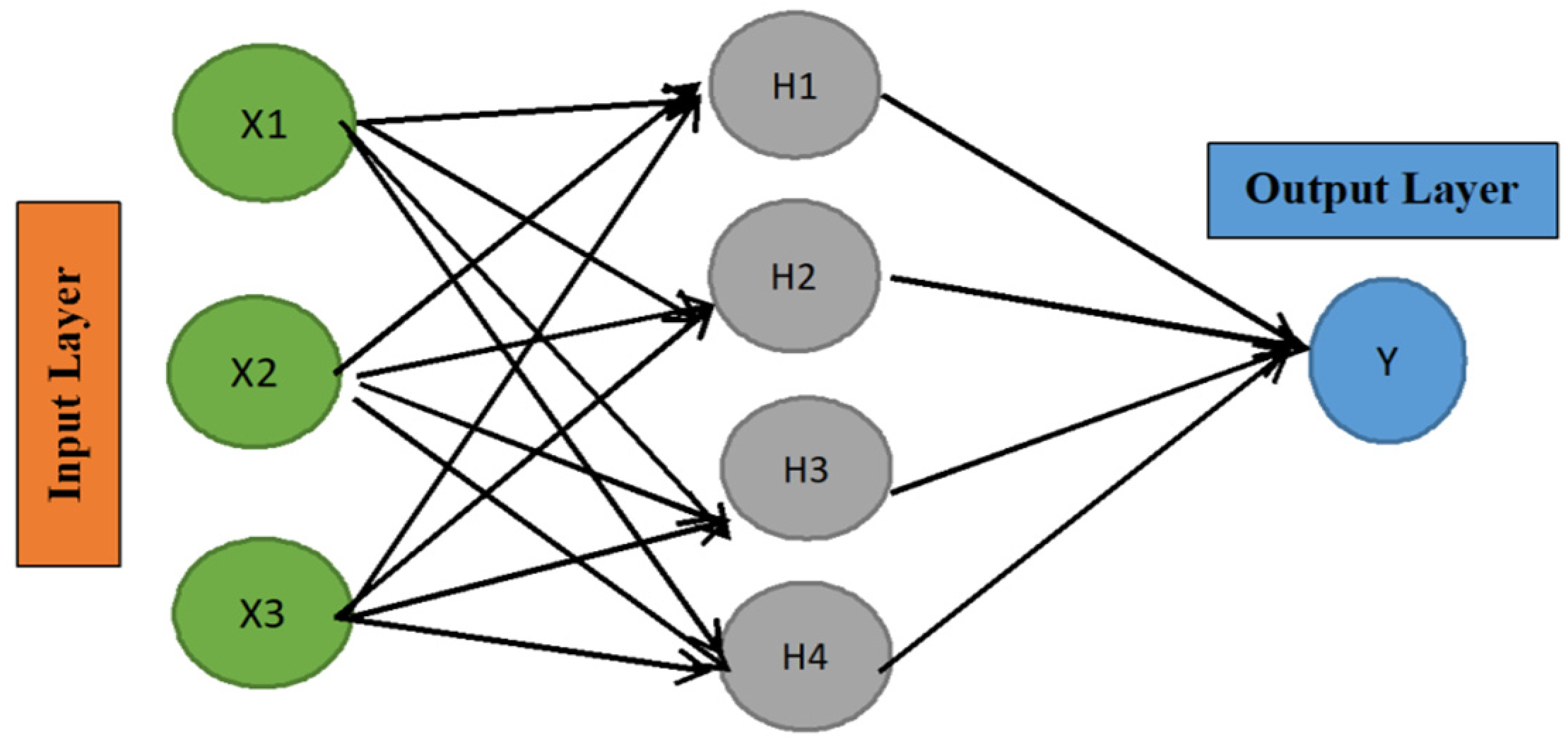
3. Multi-Layer Perceptron

The MLP is one of the widely used artificial neural networks and is applied in pattern recognition, classification, and prediction. It is classified as a Feed-Forward ANN that has the ability to map sets of input data to output data. The MLP network processes data unidirectionally throughout the network, where data points are first passed to the input layer, then processed by one or more hidden layers, and then returned through the output layer, as schematized in Figure 1. The data flow in the forward direction from input to output layer and the neurons are trained with the backpropagation learning algorithm. The required tasks, such as prediction and classification, are performed by the output layer. The neurons that process the data points in each layer, except for the input layer, receive all of the outputs from the previous layer, multiplying them by the corresponding weights, then sum all of the resulting values, and input this sum into an activation function to create the output of the neuron. The activation function, in each training iteration, will always progress forward and never revisit neurons they have encountered before, see Zell et al. (1998). Furthermore, by using feed forward neural networks, it is assumed that all input data instances are independent.

The MLP is composed of neurons called perceptions. The perceptron receives features as input ($X=\left(X_1,X_2,X_3\right))$, and each of these features is associated with a weight. Input features must be numeric and are passed as input to compute the weighted sum, as follows:

$$S\left(x\right)={\displaystyle \sum }_{\mathrm{i}=1}^{\mathrm{n}}{w}_{ij}{X}_i.$$

where $w_{ij}$ is the weight connecting neuron i to neuron j over two consecutive layers. The weighted summation is then passed as input to activation function $f$, which will produce the output of the perceptron. The activation function used in the hidden layer is the sigmoid/logistic function:

$$f\left(x\right)=\frac{1}{1+e^{-x}}$$

In the output layer, we use the softmax activation function as we have binary classification.

3.1. Learning Parameters

Connections among neurons are associated with a set of weights ($w_{ij})$ and network learning occurs by adjusting these weights in a specific manner. The backpropagation algorithm is the most commonly used learning algorithm, which consists of a forward pass and a backward pass. The backpropagation algorithm enables the MLP to update all of its weights by minimizing output error $E\left(w_{ij}\right)$in the chain rule, as given by Equation (2). In the backward pass, the error term is calculated by finding the difference between the actual response of the network and the desired response. The weights are adjusted by making the actual response of the network to be as close as possible to the desired response, and they are updated according to the general rule:

$$w_{ij}\left(t+1\right)=w_{ij}\left(t\right)-ϵ\frac{\partial E\left(w_{ij}\right)}{\partial w_{ij}}{|}_{w_{ij}=w_{ij}\left(t\right)}$$

(1)

$$\frac{\partial E\left(w_{ij}\right)}{\partial w_{ij}}=\frac{\partial E\left(w_{ij}\right)}{\partial {\mathrm{S}}_{\mathrm{i}}}.\frac{\partial {\mathrm{S}}_{\mathrm{i}}}{\partial {\mathrm{net}}_{\mathrm{i}}}.\frac{\partial {\mathrm{net}}_{\mathrm{i}}}{\partial w_{ij}}$$

(2)

where $w_{ij}$ is the weight from neuron $j$ to neuron $i$, ${\mathrm{S}}_{\mathrm{i}}$ is the output, ${\mathrm{net}}_{\mathrm{i}}$ is the weighted sum of the inputs of neuron $i$, and t is the iteration index. This can be achieved by the gradient descent algorithm, which make use of learning rate $ϵ$ to decide the step length toward the minimum for each iteration. A very small learning rate requires more training time, while a larger learning rate can produce larger weight changes on each epoch, which might cause the network to learn faster. But a larger learning rate can also lead to oscillations that prevent the error from reaching its minimum. Ideally, one would prefer to choose the largest possible learning rate without triggering oscillations. One method that has been proposed in the literature by Riedmiller and Braun (1993) is to slightly modify the backpropagation algorithm by introducing momentum term $\mu ,$ as given by Equation (4) in Agahian and Akan (2022):

$$\mathrm{\Delta }{w}_{ij}\left(t\right)=ϵ\frac{\partial E}{\partial w_{ij}}\left(t\right)+\mu \mathrm{\Delta }{w}_{ij}\left(t-1\right)$$

(3)

The momentum term decides how much the previous weight value affects the current weight update. The addition of the momentum term enables less oscillation in areas where the gradient values are similar in many directions. However, despite the fact that this parameter makes the learning process stable, in practice it has been shown that the optimal choice of this parameter is equally problem-dependent as the learning rate. Most neural network software programs provide default values for the learning rate and momentum that typically work well. Initial learning rates in the literature are found to vary widely from 0.1 to 0.9.

3.2. Resilient Propagation (Rprop)

In an attempt to find better learning parameters, appropriate adaptive weight updates have been proposed. One of the most efficient is the resilient backpropagation algorithm (Rprop) introduced as new learning scheme by Werbos (1989), which performs a direct adaptation of the weight step based on local gradient information. The Rprop was proposed to overcome the inherent disadvantages of pure gradient descent, and it is a direct adaptive method for faster backpropagation learning. The Rprop introduces an individual update value for each weight (${\mathrm{\Delta }}_{ij}),$ which increases or decreases at each iteration when multiplied by asymmetric factor ${\eta }^{+}$ or ${\eta }^{-}$ according to the sign of the gradient with respect to $w_{ij}$ between two iterations, as stated by the following learning rule:

$${\mathrm{\Delta }}_{ij}^{\left(t\right)}=\left\{\begin{array}{c}{\eta }^{+}\ast {\mathrm{\Delta }}_{ij}^{\left(t-1\right)} , if \frac{\partial E^{\left(t-1\right)}}{\partial {\omega }_{ij}}\ast \frac{\partial E^{\left(t\right)}}{\partial {\omega }_{ij}}>0\\ {\eta }^{-}\ast {\mathrm{\Delta }}_{ij}^{\left(t-1\right)} , if \frac{\partial E^{\left(t-1\right)}}{\partial {\omega }_{ij}}\ast \frac{\partial E^{\left(t\right)}}{\partial {\omega }_{ij}}<0\\ {\mathrm{\Delta }}_{ij}^{\left(t-1\right)}, else \end{array}\right\}$$

where $0<{\eta }^{-}<1<{\eta }^{+}$, $w_{ij}$ is the weight from neuron $\mathrm{j}$ to neuron $i$, and E^(t) is the t^th derivative of an arbitrary error function.

Hence, every time the partial derivative of error $E$ with respect to weight ${\omega }_{ij}$ changes it sign, this indicates that the last update was too big and the algorithm has jumped over a local minimum, and update value ${\mathrm{\Delta }}_{ij}$ is decreased by factor ${\eta }^{-}$. If the derivative retains its sign, the update value is slightly increased in order to accelerate convergence. A complete illustration of the Rprop algorithm is given by Riedmiller and Braun (1993).

3.3. Evaluation Measures

Choosing the right metric is crucial in evaluating neural network models. Various metrics are proposed in different applications. They are used to monitor and measure the performance of a model, and in our case, there are metrics available to evaluate our classification model. We use tenfold cross-validation, which is a standard way to measure the performance of the learning scheme on a particular dataset. The performance of the classifier is evaluated by using several metrics introduced and discussed in Metz (1978), Zell et al. (1998), Mas (2018), Powers (2020), and Bakhshande et al. (2022). They are labelled as follows, where (TP) indicates the number of true positives, (FP) is the number of false positives, (TN) is the number of true negatives, and (FN) is the number of false negatives. We also consider the following performance metrics as defined in McClelland et al. (1986), Metz (1978), and Powers (2020):

-

Recall, also called sensitivity, is the true positive rate (TP rate) or the probability of detection. This metric computes the proportion of actual positives that are correctly identified as such and is given by the formula:

$$\mathrm{Recall}=\frac{\mathrm{TP}}{\mathrm{TP}+\mathrm{FN}}$$

-

Specificity is also referred to as the true negative rate (TN rate). It computes the proportion of actual negatives that are correctly identified as such, as given in the formula:

$$\mathrm{Specificity}=\frac{\mathrm{TN}}{\mathrm{TN}+\mathrm{FP}}$$

-

Precision is the positive predictive value, computed by the formula:

$$\mathrm{Precision}=\frac{\mathrm{TP}}{\mathrm{TP}+\mathrm{FP}}$$

-

False positive rate (FPrate), also referred to as type I error, is given in the formula:

$$\mathrm{FPrate}=\frac{\mathrm{FP}}{\mathrm{FP}+\mathrm{TN}}=1-\mathrm{TNrate}$$

-

False negative rate (FNrate), also referred to as type II error, is given in the formula:

$$\mathrm{FNrate}=\frac{\mathrm{FN}}{\mathrm{FN}+\mathrm{TP}}=1-\mathrm{TPrate}$$

-

The F-measure, also called the F-score, is the harmonic mean of precision and sensitivity and is given by the formula:

$$\mathrm{F}-\mathrm{measure}=2\ast \frac{\mathrm{Precision}\ast \mathrm{Sensitivity}}{\mathrm{Precision}+\mathrm{Sensitivity}}$$

with the worst value = 0 and the best value = 1.

-

Matthews correlation coefficient (MCC) is a measure of the quality of the binary classification and is given by the formula:

$$\mathrm{MCC}=\frac{\mathrm{TP}\ast \mathrm{TN}-\mathrm{FP}\ast \mathrm{FN}}{\sqrt{\left(\mathrm{TP}+\mathrm{FP}\right)\left(\mathrm{TP}+\mathrm{FN}\right)}\left(\mathrm{TN}+\mathrm{FP}\right)\left(\mathrm{TN}+\mathrm{FN}\right)}$$

It ranges between −1 and +1, and it reaches −1 for perfect misclassification and +1 for perfect classification.

-

Accuracy (ACC) is the measure of the proportion of correct predictions among the total number of cases examined, as shown in the formula:

$$\mathrm{ACC}=\frac{\mathrm{TP}+\mathrm{TN}}{\mathrm{P}+\mathrm{N}}=\frac{\mathrm{TP}+\mathrm{TN}}{\mathrm{TP}+\mathrm{TN}+\mathrm{FP}+\mathrm{FN}}$$

where P and N are the total cases labeled as positive and negative, respectively.

-

The area under the ROC curve (AUC). The ROC is a popular graphical performance measure for binary classifiers. The ROC curve is plotted with TPrate against FPrate, where TPrate is on the y-axis and FPrate is on the x-axis. The higher the AUC, the better the model is at predicting 0 classes as 0 and 1 classes as 1.

-

The kappa-like statistic is discussed in Zell et al. (1998). In the traditional 2 × 2 confusion matrix employed in machine learning to evaluate the accuracy of binary classifications, the Cohen’s Kappa formula can be written as follows:

$$\mathrm{k}=\frac{2\ast \left(\mathrm{TP}\ast \mathrm{TN}-\mathrm{FN}\ast \mathrm{FP}\right)}{\left(\mathrm{TP}+\mathrm{FP}\right)\ast \left(\mathrm{FP}+\mathrm{TN}\right)+\left(\mathrm{TP}+\mathrm{FN}\right)\ast \left(\mathrm{FN}+\mathrm{TN}\right)}$$

If the original values show great similarity with the expected values, then $\mathrm{k}=1$. If there is no similarity, then $\mathrm{k}=$ 0.

4. Results

4.1. Data Description

The dataset is made up of four time series variables all of the same size (2026 observations) collected from the stock market (Tadawul) in Saudi Arabia. The data frequency was daily over the period Oct 2011 to Dec 2019. The observations were collected on a daily basis and no data were collected on Saudi bank holidays, see Rashedi et al. (2021).

Table 1. Descriptive statistics of the dataset from the Saudi stock market.

Measurements	Stock Prices	Inflation	Repo	Loil
Size	2026	2026	2026	2026
Mean	7736.387	0.016	0.696	4.299
Std. dev.	1156.632	0.02	0.28	0.354
Minimum	5416.47	−0.032	0.127	3.328
Maximum	11149.36	0.053	4.549	4.838

gives the descriptive statistics of this dataset. We believe that the macroeconomic variables Inflation, Repo, and Loil are nonstationary time series that have strong effects on the stock returns.

4.1.1. Correlations

Table 2. The correlations between the independent and dependent variables.

Variables	Closed Prices	Inflation	Repo	Loil
Closed prices	1
Inflation	−0.732	1
Repo	−0.251	0.061	1
Loil	−0.556	0.501	0.327	1

gives the correlations between these variables, which is a measure of the degree of mutual association between two or more variables. The values in Table 2 show that the closed prices are correlated with all other variables and they move together over time, which raises a question about their long-run relationship. In order to test this long-run relationship, we use the cointegration test to check for the existence of such a relationship.

4.1.2. Engle and Granger Cointegration Test

The Engle Granger test is a test for cointegration used to find a possible correlation between two or more nonstationary time series in the long term. The test is based on the idea that if variables are cointegrated, then the residual of the cointegrating regression should be stationary. The test compares the null hypothesis of no cointegration against the alternative of cointegration using static regression. Without going into more details, we use this test to analyze the relationship between the closed prices and all of the other variables. In the first step of the test, we make use of the residuals and check for the existence of unit roots. If the time series are cointegrated, the residuals would be almost stationary. In the second step, the Error Correction Model is estimated assuming the following data and equation, see Engle and Granger (1987):

$$\mathrm{\Delta }{Y}_t=c+{{\displaystyle \sum }}_{i=1}{\beta }_i\ast \mathrm{\Delta }{Y}_{t-i}+{{\displaystyle \sum }}_{i=1}{\alpha }_i\ast \mathrm{\Delta }{X}_{t-i}+\varphi \ast EC{T}_{t-1}+{\epsilon }_t$$

(4)

where $Y_t$ is the dependent variable (stock close price), $X_t$ is an independent variable, $\mathrm{\Delta }{Y}_t=Y_t-Y_{t-1}$, $\mathrm{ECT}$ is the Error Correction, and ${\epsilon }_t$ is the error term assumed to be the standard Gaussian distribution. ${\beta }_i$ and ${\alpha }_i$ are the regression parameters; and $\varphi$ is the adjustment coefficient, which must be negative. For illustration, by setting $Y_t=\mathrm{Stock}\mathrm{Price}$ and $X_t=\mathrm{Inflation}$, we obtain the corresponding Equation (4):

$$\mathrm{\Delta }{\mathrm{StockPrice}}_t=c+{\displaystyle \sum }_{i=1}{\mathsf{\beta }}_{\mathrm{i}}\ast \mathrm{\Delta }{\mathrm{StockPrice}}_{t-i}+{\displaystyle \sum }_{i=1}{\alpha }_i\ast \mathrm{\Delta }{\mathrm{Inflation}}_{t-i}+\mathrm{\varphi }{\ast \mathrm{ECT}}_{t-1}+{\epsilon }_t$$

Rejection of the null hypothesis would mean that the independent variables are causing the dependent variable.

Table 3. Engle and Granger Causality test.

Variables	Estimate	Std.Error	t-Stat (ϕ)	p-Value	R-Squared	Causality Detection
Inflation	−0.88575	0.02925	−30.286	<2 × 10−16	0.4331	Causality
Repo	−0.89178	0.02930	−30.436	<2.2 × 10−16	0.4348	Causality
Loil	−0.88806	0.02927	−30.343	<2 × 10−16	0.4338	Causality

summarizes the output of the Engle and Granger test, which indicates that, at a significance level of 5%, the independent variables are cointegrated with the dependent variable. This supports the evidence that the dependent variable closed prices is strongly affected by the movement of the independent variables Inflation, Repo, and Loil. Therefore, these variables must be included in the study.

4.1.3. Multiple Regression Model

Another statistical method that can be used to analyze the relationship between the closed prices and the other independent variables is multiple regression. The aim of this analysis is to use the independent variables to predict the value of the dependent variable. The weights or parameters are the relative contribution of each independent variable to the overall prediction, as defined by the following equation:

$$Y_i=\alpha +{{\displaystyle \sum }}_{i=1}^n{\beta }_i{X}_i+{\epsilon }_i$$

(5)

where $Y_i$ is the $i$-th observation of the logarithm of the dependent variable closed prices, and $X_i, i=1,2,\dots ,n$ are the independent variables. $\alpha$ and ${\beta }_i,i=1,2,\dots ,n$ are the regression parameters, and ${\mathsf{\epsilon }}_{\mathrm{i}}$ is an unobserved error variable.

Table 4. Regression parameter estimates of model (4) using the OLS.

Dependent Variable	Independent Variables	OLS
		Estimate	Std.Error	T-Stat
	Intercept	9.5017	0.0278	341.4130 ***
Ln(Closed prices)	Inflation	−4.4809	0.1185	−37.8010 ***
	Repo	−0.0683	0.0077	−8.8990 ***
	Loil	−0.1020	0.0070	−14.5850 ***
	R-square/Adjusted R-square	0.6203/0.6197
	F-stat.	1102 ***

Signif. codes: *** 0.01, ** 0.05, * 0.1.

shows the effect of the independent variables on the logarithm of the closed prices using the Ordinary Least Square method (OLS). The results show that the independent variables have significant negative effects on the closed prices at a significance level less than 1%.

The R-square and adjusted R-square values are 62.03% and 61.97%, respectively. Hence, the multiple regression model once again supports our claim that the variables Inflation, Repo, and Loil have direct causal effects on the closed prices.

4.2. Outlier Detection

4.2.1. Tukey Method

In this study, we use the Tukey method as the simple traditional method to provide input to the MLP algorithm. We use the upper and lower fences that are built on the Interquartile Range (IQR), which is the difference between the third quartile (Q3) and the first quartile (Q1), thus IQR = Q3 − Q1. Outliers are defined as observations that lie outside the interval [Q1 − 3IQR, Q3 + 3IQR], whereas observations that fall 1.5 times the interquartile range away from the first and third quartiles, [Q1 − 1.5IQR, Q3 + 1.5IQR] are regarded as suspected outliers.

The outliers are first detected in the return data using the Tukey method based on the upper and lower fences. These computed values are respectively 0.01908 and −0.01783, and they are shown in Figure 2. Any return value that is outside the band delineated by the dashed lines is regarded as an outlier.

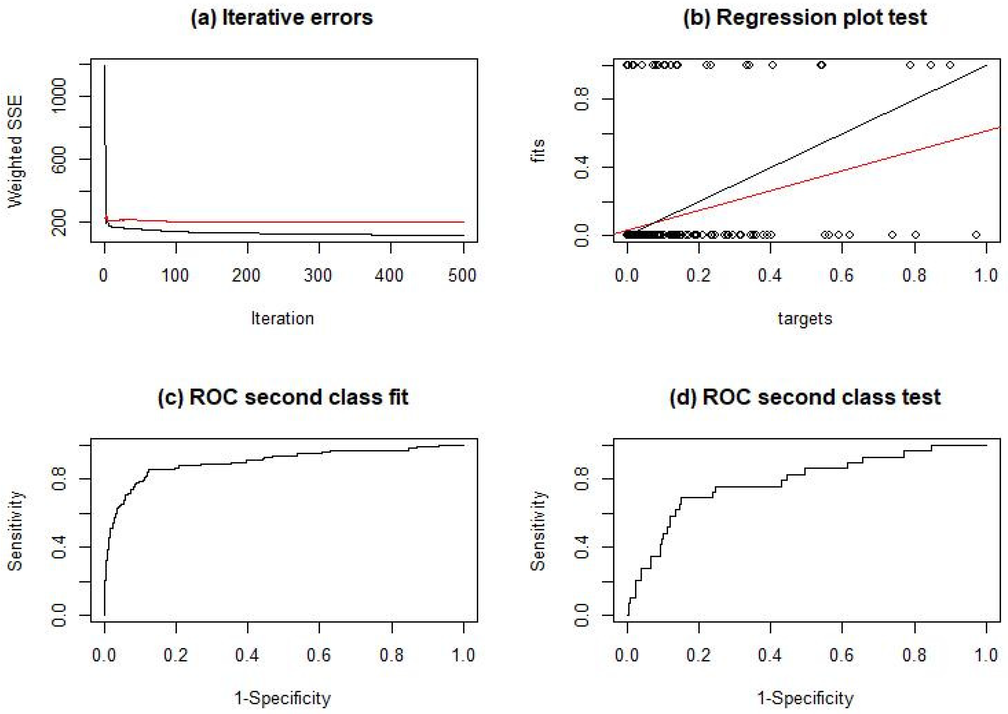
4.2.2. MLP Evaluation

In order to classify whether a data point from the return series is an outlier, we run the MLP algorithm. The package used for creating the actual MLP in R is called RSNNS, which is an R-wrapper for the Stuttgart Neural Network Simulator (SNNS), refer to Bergmeir and Benítez Sánchez (2012). We split our dataset into 80% training (1622 observations) and 20% testing (405 observations). As input to the MLP network, we use three input neurons, 50 hidden neurons, and set the learning function to Rprop with 0.001 for the learning function parameter. The input neurons accept the values of the three variables Inflation, Repo, and Loil, while the expected value of the output neuron is either 0 or 1. In the running of the MLP model, we used the Rprop algorithm with the iterations n = 500, 1000, and 1500.

Table 5. Performance measure of the MLP model using different metrics.

Iterations	Sample	Matrix			TP Rate	TN Rate	FP Rate	FN Rate
			No Outliers	Outliers
n = 500	Train (80%)	No outliers	1511	93	0.9420	0.7222	0.2778	0.0580
		Outliers	5	13
	Test (20%)	No outliers	378	20	0.9497	0.2857	0.7143	0.0503
		Outliers	5	2
n = 1000	Train (80%)	No outliers	1510	76	0.9521	0.8571	0.1429	0.0479
		Outliers	5	30
	Test (20%)	No outliers	378	19	0.9521	0.3750	0.6250	0.0479
		Outliers	5	3
n = 1500	Train (80%)	No outliers	1511	76	0.9521	0.8571	0.1429	0.0479
		Outliers	5	30
	Test (20%)	No outliers	376	19	0.9519	0.3000	0.7000	0.0481
		Outliers	7	3

and

Table 6. Some statistical criteria for detecting outliers.

Iterations	Sample	ACC	ROC Area	MCC	Precision	F-Score	Cohen’s Kappa
n = 500	Train (80%)	0.9396	0.8321	0.2816	0.9967	0.9686	0.1944
	Test (20%)	0.9383	0.6177	0.1354	0.9869	0.9680	0.1147
n = 1000	Train (80%)	0.9500	0.9046	0.4758	0.9967	0.9739	0.4063
	Test (20%)	0.9407	0.5617	0.2008	0.9869	0.9692	0.1761
n = 1500	Train (80%)	0.9501	0.9046	0.4758	0.9967	0.9739	0.4063
	Test (20%)	0.9358	0.5590	0.1725	0.9817	0.9666	0.1589

show the different evaluation measures, as defined in Section 3.3, to measure the MLP performance in classifying the input data. Table 5 shows that in the 80% training data, the TP rate increases from 94.2% with n = 500 to 95.21% with n = 1500, and the TN rate increases from 72.22% with n = 500 to 85.71% with n = 1500. At the same time, the FP rate decreases from 27.78% with n = 500 to 14.29% with n = 1500, and the FN rate decreases from 5.80% with n = 500 to 4.79% with n = 1500. Table 5 also shows these numbers for the 20% data test sample. In the test data, the TP rate is around 95% for all iterations, while the TN rate fluctuates between 28.57% and 37.50% from n = 500 to n = 1500. The FP rate decreases from 70.0% to 62.5%, then back to 70% for n = 500, 1000, and 1500, and the FN rate shows a slight decrease from 5.03% with n = 500 to 4.81% with n = 1500.

Table 6 summarizes the other criteria that measure the performance of the MLP. In the 80% training sample, the performance measure criteria ACC remains slightly over 93%. The ROC area increases from 83.21% with n = 500 to 90.46% with n = 1500, the MCC increases from 28.16 to 47.58%, and similarly, the F-score and Cohen’s Kappa increase when the number of iterations increases from n = 500 to n = 1500. Table 6 also shows the results of these measures in the 20% data test sample. In this test sample, the ACC fluctuates around 93.0% and the ROC area shifts up to 61% and down to 55.9%. On the other hand, the Precision and F-score remain nearly unchanged and their values are respectively around 98% and 96%. Finally, the MCC and Cohen’s Kappa respectively shift up and down between 13.5% and 20% and between 11.5% and17.6%.

Figure 3, plot (a) shows the weighted sum square error (SSE), with the iterative fit error as the black line and the iterative test error as the red line. As can be seen, both lines strongly decrease over the first few iterations, then their values stay steady around 200, demonstrating that the algorithm quickly converges. After properly training the model, we make predictions and plot the regression errors in (b), where the target values are on the x-axis and the predicted values are on the y-axis. In the optimal fit, we would have a line through zero with a gradient of one. This optimal line is shown in black and the linear fit to the actual data is shown in red.

To further evaluate the network performance, we plot the ROC curves for both phases, showing the training set in (c) and test set in (d). The ROC is a metric used to check the quality of classifiers. For each class of a classifier, the ROC applies threshold values across the interval [0, 1] to the outputs. The ROC curve is a plot of the TPrate against the FPrate, where the FPrate is on the x-axis and the TPrate is on the y-axis. A perfect test would show points in the upper-left corner, with 100 percent sensitivity and 100 percent specificity. The more we have a top left side ROC curve, the better is the classifier and the better is the network performance.

5. Conclusions

The main purpose of this research work was to explore the MLP neural network algorithm in detecting outlier values in the daily returns of the Saudi Stock Market (Tadawul). The dataset under study comprised four times series variables, including the closed prices, inflation rate, repo rate, and oil prices. In Section 4.1.1 and Section 4.1.2, we showed that the closed prices were correlated with the other variables, and the Engle Granger test for cointegration was carried out and confirmed the long-run relationship that existed between these variables. This claim was again confirmed in Section 4.1.3, using multiple linear regression fit, where the logarithm of the closed prices was the dependent variable. This finding showed that the closed prices were strongly and directly affected by the remaining variables. This suggested the need to consider all of the independent variables when searching for outliers in the closed prices. Because we wanted to apply the MLP model to detect outliers, we first needed to run a simple method, like the traditional Tukey method, to find these outliers and then input them when running the MLP algorithm. In an attempt to achieve our goal, we proposed a novel MLP model to detect and classify outlier values based on independent variables without referring to stock return data. The performance of our MLP based procedure was evaluated using various test criteria, such as the false positive rate (FPrate), false negative rate (FNrate), F-measure, Matthews correlation coefficient (MCC), accuracy (ACC), and ROC curves. The obtained results over the training sample showed that the performance of the MLP was efficient based on these criteria and under different iteration numbers: n = 500, 1000, and 1500. In addition, this study showed that running the MLP with the Rprop over the test sample was capable of detecting and classifying future outlier values in Tadawul. This study shows and demonstrates the usefulness of the MLP neural network in detecting outliers in a multivariate dataset. It is important to note a crucial difference between the Tukey method and the MLP method. The Tukey procedure was only applied on the univariate data, which were the returns, while the MLP-based method operated on the multivariate data made up of the three variables.

We should point out that although our methodology was demonstrated on the Tadawul dataset, it can be applied to other similar datasets within the context of binary classification. However, this study has several limitations that should be acknowledged. Firstly, the analysis focused on a limited set of input variables, namely inflation, repo rate, and oil prices, for outlier detection in stock returns. There are other factors that could be taken into account, such as economic indicators and market sentiment or global events, which could also influence stock returns. Secondly, the dataset used in this study was limited to a specific timeframe, potentially limiting the generalization of the findings. This issue could be addressed in future studies when the dataset is updated. Additionally, while the study focused on the Multi-Layer Perceptron (MLP) algorithm, comparing the performance of other outlier detection models, such as support vector machine, random forest, or deep learning models, would provide a more comprehensive understanding of their effectiveness in detecting stock return outliers.

References

1. Agahian, Saeid, and Taymaz Akan. 2022. Battle royale optimizer for training multi-layer perceptron. Evolving Systems 13: 563–75. [Google Scholar] [CrossRef]
2. Al-Saif, Adel M., Mahmoud Abdel-Sattar, Abdulwahed M. Aboukarima, and Dalia H. Eshra. 2021. Application of a multilayer perceptron artificial neural network for identification of peach cultivars based on physical characteristics. PeerJ 9: e11529. [Google Scholar] [CrossRef]
3. Bakhshande, Fateme, Daniel Adofo Ameyaw, Neelu Madan, and Dirk Söffker. 2022. New Metric for Evaluation of Deep Neural Network Applied in Vision-Based Systems. Applied Sciences 12: 3251. [Google Scholar] [CrossRef]
4. Bani-Salameh, Hani, Shadi M. Alkhatib, Moawyiah Abdalla, Mo’taz Al-Hami, Ruaa Banat, Hala Zyod, and Ahed J. Alkhatib. 2021. Prediction of diabetes and hypertension using multi-layer perceptron neural networks. International Journal of Modeling, Simulation, Scientific Computing 12: 2150012. [Google Scholar] [CrossRef]
5. Bergmeir, Christoph Norbert, and José Manuel Benítez Sánchez. 2012. Neural networks in R using the Stuttgart neural network simulator: RSNNS. Journal of Statistical Software 46. [Google Scholar] [CrossRef]
6. Boughaci, Dalila, Abdullah A. K. Alkhawaldeh, Jamil J. Jaber, and Nawaf Hamadneh. 2021. Classification with segmentation for credit scoring and bankruptcy prediction. Empirical Economics 61: 1281–309. [Google Scholar] [CrossRef]
7. Chen, Jinghui, Saket Sathe, Charu Aggarwal, and Deepak Turaga. 2017. Outlier detection with autoencoder ensembles. Paper presented at SIAM International Conference on Data Mining, Houston, TX, USA, April 27–29; pp. 90–98. [Google Scholar]
8. Engle, Robert F., and Clive W. J. Granger. 1987. Co-integration and error correction: Representation, estimation, and testing. Econometrica: Journal of the Econometric Society 55: 251–76. [Google Scholar] [CrossRef]
9. Gouda, Walaa, Sidra Tahir, Saad Alanazi, Maram Almufareh, and Ghadah Alwakid. 2022. Unsupervised Outlier Detection in IOT Using Deep VAE. Sensors 22: 6617. [Google Scholar] [CrossRef] [PubMed]
10. Hounmenou, Castro Gbememali, Kossi Essona Gneyou, and Romain Lucas Glele Kakaï. 2021. A Formalism of the General Mathematical Expression of Multilayer Perceptron Neural Networks. Preprints, 2021050412. [Google Scholar] [CrossRef]
11. Kaastra, Iebeling, and Milton J. Boyd. 1996. Designing a neural network for forecasting financial and economic time series. Neurocomputing 10: 215–36. [Google Scholar] [CrossRef]
12. Mas, Jean-François. 2018. Receiver operating characteristic (ROC) analysis. In Geomatic Approaches for Modeling Land Change Scenarios. Cham: Springer, pp. 465–67. [Google Scholar]
13. McClelland, James L., David E. Rumelhart, and Geoffrey E. Hinton. 1986. The Appeal of Parallel Distributed Processing. Cambridge: MIT Press, Volume 3, p. 44. [Google Scholar]
14. Metz, Charles E. 1978. Basic principles of ROC analysis. Seminars in Nuclear Medicine 8: 283–98. [Google Scholar] [CrossRef] [PubMed]
15. Powers, David M. W. 2020. Evaluation: From precision, recall and F-measure to ROC, informedness, markedness and correlation. arXiv arXiv:2010.16061. [Google Scholar] [CrossRef]
16. Rashedi, Khudhayr A., Mohd Tahir Ismail, Nawaf N. Hamadneh, S. Al Wadi, Jamil J. Jaber, and Muhammad Tahir. 2021. Application of radial basis function neural network coupling particle swarm optimization algorithm to classification of Saudi Arabia stock returns. Journal of Mathematics 2021: 5593705. [Google Scholar] [CrossRef]
17. Riedmiller, Martin, and Heinrich Braun. 1993. A direct adaptive method for faster backpropagation learning: The RPROP algorithm. Paper presented at IEEE International Conference on Neural Networks, San Francisco, CA, USA, March 28–April 1; pp. 586–91. [Google Scholar]
18. Rosenblatt, Frank. 1958. The perceptron: A probabilistic model for information storage and organization in the brain. Psychological Review 65: 386. [Google Scholar] [CrossRef] [PubMed]
19. Saha, Sunil, Gopal Chandra Paul, Biswajeet Pradhan, Khairul Nizam Abdul Maulud, and Abdullah M Alamri. 2021. Integrating multilayer perceptron neural nets with hybrid ensemble classifiers for deforestation probability assessment in Eastern India. Geomatics, Natural Hazards Risk 12: 29–62. [Google Scholar] [CrossRef]
20. Sathe, Saket, and Charu Aggarwal. 2016. LODES: Local Density Meets Spectral Outlier Detection. Paper presented at 2016 SIAM International Conference on Data Mining (SDM), Miami, Florida, USA, May 5–7. [Google Scholar]
21. Tukey, John W. 1977. Exploratory Data Analysis. Volume 2, pp. 131–60. [Google Scholar]
22. Werbos, P. 1989. Back-propagation and neurocontrol: A review and prospectus. In Paper presented at IEEE Proceedings of the International Joint Conference on Neural Networks (IJCNN’89); pp. 209–16. [Google Scholar]
23. Zell, A., G. Mamier, M. Vogt, N. Mache, R. Hübner, S. Döring, K. Herrmann, T. Soyez, M. Schmalzl, and T. Sommer. 1998. SNNS: Stuttgart Neural Network Simulator. User Manual, Version 4.2. Technical Report (6/95). Institute for Parallel Distributed High Performance Systems. [Google Scholar]
24. Zurada, Jacek. 1992. Introduction to Artificial Neural Systems. St Paul: West Publishing Co. [Google Scholar]
Figure 1. Simple Multi-Layer Perceptron ANN. All nodes of the input layer are connected to nodes in the hidden layer. The output layer takes input from the last hidden layer to produce prediction based on the model learning.
Jrfm 17 00069 g001
Figure 2. Blue line is the ordered return, and values outside of the upper and lower fences (dash line) are considered as outliers.
Jrfm 17 00069 g002
Figure 3. (a) Plot of the iterative fit error (black) and the iterative test error (red). (b) The regression plot for the test data. For an ideal classification, only the points (0, 0) and (1, 1) would be populated. (c) ROC plot for the second class against all other classes in the training set. (d) same as (c), but for the test data.
Jrfm 17 00069 g003