
Abstract
Deep Neural Networks (DNN) have made significant advances in various fields including speech recognition and image processing. Typically, modern DNNs are both compute and memory intensive, therefore their deployment in low-end devices is a challenging task. A well-known technique to address this problem is Low-Rank Factorization (LRF), where a weight tensor is approximated by one or more lower-rank tensors, reducing both the memory size and the number of executed tensor operations. However, the employment of LRF is a multi-parametric optimization process involving a huge design space where different design points represent different solutions trading-off the number of FLOPs, the memory size, and the prediction accuracy of the DNN models. As a result, extracting an efficient solution is a complex and time-consuming process. In this work, a new methodology is presented that formulates the LRF problem as a (FLOPs vs. memory vs. prediction accuracy) Design Space Exploration (DSE) problem. Then, the DSE space is drastically pruned by removing inefficient solutions. Our experimental results prove that the design space can be efficiently pruned, therefore extract only a limited set of solutions with improved accuracy, memory, and FLOPs compared to the original (non-factorized) model. Our methodology has been developed as a stand-alone, parameterized module integrated into T3F library of TensorFlow 2.X.
1 Introduction
In recent years, the world has witnessed the revolution of Artificial Intelligence (AI), especially in the fields of Machine Learning (ML) and Deep Learning (DL), attracting the attention of many researchers in various application fields [1]. Such an example is the Internet-of-Things (IoT) ML-based applications, where DNNs are employed on edge devices that are characterized by limited compute and memory capabilities [2].
State-of-the-art DNN models consist of a vast number of parameters (hundreds of billions) and require trillions of computational operations not only during the training, but also at the inference phase [3]. Therefore, executing these models on Resource-Constrained Devices (RCD), e.g., edge and IoT devices, is a challenging task. The problem becomes even more challenging when the target applications are characterized by specific real-time constraints [4]. To address this problem, many techniques have been recently proposed to compress and accelerate DNN models [5, 6]. DNN compression methods reduce both the number of arithmetical tensor operations and the memory size of the model, without significantly impacting its accuracy. In general, DNN compression techniques are classified into five main categories [6]: pruning [7], quantization [8], compact convolutional filters [9], knowledge distillation [10], and low-rank factorization [11].
Pruning techniques reduce the complexity of DNN models by removing unnecessary elements [7], e.g., neurons or filters [12,13,14]. Quantization is a well-studied technique targeting to transform the 32-bit Floating-Point (FP32) weights and/or activations into less-accurate data types, e.g., Integer8 (INT8) or FP16 [8]. In the compact convolutional filter techniques, special structural convolutional filters are designed to reduce the size of the convolution filters and therefore reduce both the number of tensor operations and the memory size [9]. Finally, knowledge distillation is the process of transferring the knowledge from a large model to a smaller one by following a student-teacher learning model [15]. The two latter techniques can be applied only to the convolutional layers [6]. On the contrary, Low-Rank Factorization (LRF) can be used to reduce both the number of Floating-Point Operations (FLOPs) as well as the memory size in both convolutional and Fully Connected (FC) layers by transforming the original tensors into smaller ones [11]. However, employing LRF in a neural network model is not a straightforward process: it includes a huge design space and different solutions provide different trade-offs among FLOPs, memory size, and prediction accuracy; therefore, finding an efficient solution is not a trivial task.
In this work, we provide a methodology to orchestrate the deployment of LRF in the FC layers of typical DNN models. We target the FC memory arrays because they typically account for the largest percentage of overall memory size of DNN models. As Fig. 1 indicates, the FC memory size ranges from 49% up to 100% of the total DNN memory size for the seven studied models.

Memory and FLOPs percentages of FC and non-FC layers for the seven studied models. The memory occupied by the FC layers is from 49% up to 100%
The steps of the proposed methodology are as follows. First, all the FC layer parameters are extracted from a given DNN model. Second, all possible LRF solutions are generated using the T3F library [16]. Then, the vast design space is pruned in two phases and a (limited) set of solutions is selected for re-evaluation/calibration according to specific target metrics (FLOPs, memory size, and accuracy) that are provided as inputs to our methodology.
The main contributions of this work are:
-
A new method that formulates the LRF problem as a (FLOPs, memory size, and accuracy) DSE problem
-
A step by step methodology that effectively prunes the design space
-
A fully parameterized and stand-alone DSE tool integrated into T3F library (part of TensorFlow 2.X [17])
-
A thorough experimental evaluation using seven popular DNN models and various datasets
This work is an extended version of our previous work presented in [18].
The rest of this paper is organized as follows: In Sect. 2, we put this work in the context of related works and present the relevant background information. The proposed methodology is presented in a step-by-step basis in Sect. 3, while the experimental results are discussed in Sect. 4. Finally, Sect. 5 is dedicated to conclusions and future work.
2 Background and Related Works
2.1 Low-Rank Factorization
LRF refers to the process of approximating and decomposing a matrix or a tensor by using smaller matrices or tensors [19]. Suppose \(M \in \mathbb {R}^{m\times n}\) is a matrix with m rows and n columns. Given a rank r, M can be approximated by \(M^{\prime} \in \mathbb {R}^{m\times n}\); \(M^{\prime}\) has a lower rank k and it can be presented by the product of two (or more) thinner matrices \(U \in \mathbb {R}^{m\times k}\) and \(V \in \mathbb {R}^{k\times n}\) with m rows/k columns and k rows/n columns, respectively (as shown in Fig. 2). The element (i, j) from M is retrieved by multiplying the i-th row of U by the j-th column of V. The original matrix M needs to store \(m\times n\) elements, while the approximated matrix \(M^{\prime}\) (using two thinner matrices U and V) needs to store \((m\times k)+(k\times n)\) elements [19].

Basic Low-Rank Factorization (LRF) in 2D matrices
To decompose the input matrices, different methods exist, such as Singular Value Decomposition (SVD) [20,21,22], QR decomposition [23, 24], interpolative decomposition [25], and non-negative factorization [26]. Given that tensors are multidimensional generalizations of matrices, they need different methods to be decomposed, e.g., Tucker Decomposition [27, 28], Canonical Polyadic Decomposition (CPD) [29, 30], and Tensor Train (TT) Decomposition [31]. Another way to decompose tensors is to transform the input tensor into a two-dimensional (2D) matrix and then perform the decomposition process using one of the above mentioned matrix decomposition techniques [32, 33].
2.2 Tensor Train Format and T3F Library
A popular method to decompose the multidimensional tensors is the TT format, proposed in [31]. It is a stable method that does not suffer from the curse of dimensionality [31]; furthermore, the number of parameters needed is similar to that in CPD [31]. A tensor \(A(j_1, j_2,\ldots, j_d)\) with d dimensions can be represented in TT format if for each element with index \(j_k = 1, 2,\ldots, n_k\) and each dimension \(k = 1, 2,\ldots, d\) there is a collection of matrices \(G_k[j_k]\) such that all the elements of A can be computed by the following product [34]:
All matrices \(G_k[j_k]\) related to the same dimension k are restricted to be of the same size \(r_{k-1}\times r_k\). The values \(r_0\) and \(r_d\) are equal to 1 in order to keep the matrix product (Eq. 1) of size \(1\times 1\).
As noted, the proposed DSE methodology is built on top of TensorFlow 2.X and integrated into T3F library as a fully parameterized, stand-alone module. T3F is a library [16] for TT-Decomposition and currently is only available for FC layers. In the current version, our target is the FC layers, because as depicted in Fig. 1, the FC layers occupy the largest memory size in typical DNN architectures. The main primitive of T3F library is TT-Matrix, a generalization of the Kronecker product [35]. By using the TT-format, T3F library compresses the 2D array of a FC layer into multiple smaller size 4D tensors by using a small set of parameters.
The inputs to the modified T3F module are: (i) the weight matrix of the original FC layer (2D array), ii) the max-tt-rank value which is the maximum rank and it defines the density of the compression; small max-tt-rank values offer higher compression rate, and (iii) a set of tensor configuration parameters. The latter set of parameters is related to the shape of the output tensors that the input 2D array is compressed; if these tensors are multiplied by each other, then the original 2D matrix can be approximated. As an example, the following set of parameters [[7, 4, 7, 4], [5, 5, 5, 5]] approximates a matrix of size \(784\times 625\). In other words, by multiplying the first set of numbers (\(7\times 4\times 7\times 4=784\)), the first dimension of the weight matrix (784) is produced and by multiplying the second set of numbers (\(5\times 5\times 5\times 5=625\)), the second dimension of the weight matrix (625) is generated.
After the decomposition is done, T3F library outputs a set of 4D tensors (called cores) with the following shapes/parameters:
where \(s_1, s_2,\ldots , s_{n-1}, s_n\) and \(o_1, o_2,\ldots , o_{n-1}, o_n\) are the aforementioned tensor configuration parameters and r is equal to the max-tt-rank parameter. In the above-mentioned example, then the generated cores become (assume that \(r=2\)):
-
Core #1 dim: (1, 7, 5, 2)
-
Core #2 dim: (2, 4, 5, 2)
-
Core #3 dim: (2, 7, 5, 2)
-
Core #4 dim: (2, 4, 5, 1).
As noted, if the above tensors are multiplied by each other, the original 2D matrix is approximated.
Finally, the number of parameters (of all cores) can be provided by:
2.3 Motivation
One of the main challenges in employing LRF for a specific DNN model is to select a suitable rank parameter [32]. Given a predefined rank value, the process of extracting the decomposed matrices or tensors is a well-defined and straightforward process. For example, the SVD algorithm [36] can used to generate the output low-rank matrix with the minimal or a pre-defined approximation error, given an input matrix and a rank value.
While many researchers devised techniques targeting to find the best rank value [32, 37,38,39], it has been proven that this is an NP-hard problem [32]. For example, assuming a max rank value of 10 in LeNet5 model [40] (LeNet5 consists of three FC layers with dimensions \(400\times 120\), \(120\times 84\), and \(84\times 10\), respectively), the entire design space contains about 252 million possible solutions to configure the decomposed matrices. Given that a model calibration phase (typically for more than three epochs) must be employed for each extracted solution, this means that \(252M\times 3\times 1\) seconds (approximately 8750 days assuming that each epoch takes about 1 second) are needed to cover the whole design space. To the best of our knowledge there is no similar work that formulates the LRF problem as a DSE problem.
3 Methodology
To address the above problem, a DSE methodology and a fully parameterized tool are proposed in this work. The target is to ease and guide the LRF process in FC layers. The main steps of the proposed methodology are shown in Fig. 3. In the rest of this section, a detailed description of each step in Fig. 3 is provided.

The proposed DSE methodology
-
1.
Extract the FC layers from the model architecture and exclude the small layers: As noted, the first step of our approach is to extract and analyze all FC layers of a given DNN model. Among all the extracted FC layers, the layers with small memory sizes with respect to the overall memory footprint of the model (based on a threshold) are discarded. The aim of LRF is to reduce the required memory size and computations, thus applying LRF to layers with meager sizes does not provide significant memory/FLOP gains. As part of this work, a threshold with a value equal to 10% (experimentally derived) is used.
-
2.
Generate all possible LRF solutions: In this step, all different LRF solutions are generated using the T3F library. The 2D input weight matrices are converted into tensors of smaller size according to TT format. Each different tensor shape represents a unique solution. Note that in the current step, each solution is extracted as a set of configuration parameters (that includes the maximum rank and the shape of the tensors) and all possible solutions are extracted for each layer individually.
Let us give an example by using a small-in-size layer from LeNet5 model and a larger layer from the well-known AlexNet model [41]. The FC layer in AlexNet has a shape equal to \(4096\times 4096\) and the shape of the FC layer in LeNet5 is equal to \(120\times 84\). In these layers, all possible rank values are considered. Figure 4 depicts all different solutions for both layers (the graph in Fig. 4a corresponds to AlexNet, while the one in the right to LeNet5). The vertical axis shows the number of FLOPs and the horizontal axis the number of parameters. Both axes are in log-scale. As it is obvious from Fig. 4 the underlying design space is huge: 7759741 different solutions for AlexNet layer and 18799 different solutions for LeNet5 layer. Finally, the black circle in each graph represents the FLOPs-memory design point of the non-factorized layer.

All possible solutions based on T3F library for a layer of size/shape equal to (a) \(4096\times 4096\) in AlexNet and (b) \(120\times 84\) in LeNet5. The black circle corresponds to the non-factorized layer
-
3.
Calculate the number of FLOPs and memory size for each solution: The mathematical expressions to calculate the required memory and FLOPs for each solution are given by Eqs. (3) and (4), respectively. In particular, assuming a FC layer with shape [X, Y], the memory size is given by the following formula:
$$\begin{aligned} Memory = \left( \left( \sum _{i=1}^{L}\prod _{j=1}^{4}c_{i,j}\right) + Y\right) \times Bytes, \end{aligned}$$(3)where L is the number of cores (length of combination), \(c_{i,j}\) is j-th element in the i-th core, and Y is the length of bias vector. As noted, LRF takes as input a 2D array and generates a number of 4D tensors (called cores). To calculate the memory size required for a layer, we need first to calculate and sum up the number of parameters for each core. Then, the bias must be added to the calculated value. Finally, to find the required memory, the number of parameters is multiplied by the size of the data type (e.g., 4 bytes for FP32). Following up the example in the previous section and based on Eq. (3), the size of the factorized layer is equal to 3820 bytes (\(((1\times 7\times 5\times 2) + (2\times 4\times 5\times 2) + (2\times 7\times 5\times 2) + (2\times 4\times 5\times 1) + 625)\times 4\)), while the size of the original (non-factorized layer) is equal to 1962500 bytes.
The number of FLOPs is given by the following formula:
$$\begin{aligned} FLOPs = \left( \sum _{i=1}^{L}\left( cl_i\times cr_i\times inr_i + \left( \prod _{j=1}^{4}c_{i,j} + cr_i\times inr_i\right) \right) \right) + Y, \end{aligned}$$(4)where \(inr_i = \prod _{j=1}^{L-1}x_j\), \(cr_i = c_{i,2}\times c_{i,4}\) (multiplication of second and last element of current core that are related to the input combination element and rank value, respectively), \(cl_i = c_{i,1}\times c_{i,3}\) (multiplication of first and third element of current core that are related to the output combination element and rank value, respectively) and \(x_j\) is j-th element in the input combination. Similarly, for the above-mentioned example, the number of calculated FLOPs is 73475 instead of 980000 FLOPs in the non-factorized case (in the first iteration, \(i=1, cr_1=14, cl_1=5,\) and \(\prod _{j=1}^{4}c_{1,j}=70\) so we have \((5\times 14\times 196 + (70 + (14\times 196)))\). In the second iteration, \(i=2, cr_2=8, cl_2=10,\) and \(\prod _{j=1}^{4}c_{2,j}=80\) so we have \((10\times 8\times 196 + (80 + (8\times 196)))\). In the third iteration, \(i=3, cr_3=14, cl_3=10,\) and \(\prod _{j=1}^{4}c_{3,j}=140\) so we have \((10\times 14\times 196 + (140 + (14\times 196)))\). In the fourth iteration, \(i=4, cr_4=4, cl_4=10,\) and \(\prod _{j=1}^{4}c_{4,j}=400\) so we have \((10\times 4\times 196 + (400 + (4\times 196)))\). Finally all the values are summed with 625);
-
4.
Prune the design space—Phase A (Discard all inefficient solutions of each FC layer): As noted, the underlying design space is vast, therefore fine-tuning or calibrating the model for all the possible solutions is not feasible. To address this problem, the FLOPs vs. memory design space (illustrated in Fig. 5) is divided into four distinct areas. The top-right part (red part in Fig. 5) is excluded for the remaining steps, since it contains solutions that require more memory and more FLOPs compared to the non-factorized (initial) solution. Note that the blue dot in the center of the graph corresponds to the memory/FLOPs of the non-factorized solution. The top-left and bottom-right parts (yellow parts in Fig. 5) are also excluded. Although the latter two parts can contain acceptable solutions, we have excluded them as the solutions in these parts require more FLOPs (top left) or more memory (bottom right) compared to the initial model. The bottom left part (green part in Fig. 5) includes solutions that exhibit less memory and less FLOPs with respect to the initial layer. As part of this work, we consider only the solutions in the green box i.e., these solutions will be forwarded to the remaining steps of our methodology.
-
5.
Prune the design space—Phase B (Formulate the baseline mapping and tiling strategy): In this step, the 2D design space (green part in Fig. 5) of each layer is further broken down into smaller rectangles (tiles) of predefined size. As a first approach [18], an \(8\times 8\) grid is considered i.e., each green rectangle in Fig. 5 is broken down into 64 tiles. In other words, the whole design space now consists of 64 tiles and each tile contains multiple solutions (note: a tile might contain no solutions). The next step is to extract one or more solutions from each tile. A straightforward way is to extract the following four solutions [18]:
-
Point 1: Min_Memory_Min_FLOPs
-
Point 2: Min_Memory_Max_FLOPs
-
Point 3: Max_Memory_Min_FLOPs
-
Point 4: Max_Memory_Max_FLOPs
-

The design space is illustrated as a (FLOPs vs. memory) pareto curve and partitioned into rectangles. The red part and yellow parts are pruned (excluded), because they contain solutions with more memory and/or more FLOPs compared to the original (non-factorized) layer (Color figure online)
Obviously, the four above mentioned solutions cover the best and worst cases in terms of FLOPs and/or memory requirements per tile. Given that there are 64 tiles, a maximum number of \(4\times 64\) solutions are extracted for each FC layer and the remaining solutions are discarded. Although this is an effective approach [18], our evaluation results reveal the following pathological issue. In many cases (tiles), the four above-mentioned solutions can coincide with each other and as a result the number of the per-tile extracted solutions is less than four (typically one or two). Figure 6 quantifies this problem for the FC layers of all studied models (horizontal axis). The vertical axis of Fig. 6 shows the percentage of tiles in which four (gray bar segments), three (red), two (blue), one (green) or zero (black) solutions are extracted from each tile. On average (rightmost bar), four solutions are selected in only 2% of the cases, while two distinct solutions are selected in 40% of the tiles. Obviously, this reported coverage can reduce the effectiveness of our methodology, since multiple "good" solutions might be omitted.

Coverage of the initial mapping strategy. The gray/red/blue/green/black bar segments correspond to the percentage of tiles in which 4/3/2/1/0 solutions are extracted
To further illustrate this problem, let us consider a tile with a set of solutions as extracted by the fourth step of the proposed methodology. The mapping strategy described so far (called Min-Max-Mapping-Strategy or MMMS hereafter) is depicted in Fig. 7a. It is obvious from Fig. 7a) that both Max_Memory_Min_FLOPs and Max_Memory_Max_FLOPs solutions will end-up to the same design point (annotated by the dark blue point). To tackle this issue, more effective mapping strategies are proposed and evaluated in the next subsection.
-
6.
Prune the design space—Phase C (Increase the per-tile coverage): The MMMS method explained in the previous section is enhanced so as more unique solutions (ideally four) are extracted for each tile. The new proposed mapping strategy, called Nearest-to-Corner-Mapping-Strategy (N2CMS), is depicted in Fig. 7b.
In N2CMS, the four solutions closest to the four corners (annotated by the four red arrows in Fig. 7b) in each tile are considered. However, N2CMS might fail as a victim of the following situation: a specific point might have exactly the same distance from two corners. For example, the yellow point in Fig. 7c has the same distance (\(L_1 = L_2\)) from the bottom right and the top right corners. The result in this case is that three (and not four) solutions are selected in the specific tile. Note that the maximum number of solutions that can be disregarded due to this behavior is two.

The three different per-tile mapping strategies: (i) the Min-Max-Mapping-Strategy (MMMS) described in step 5, (ii) the Nearest-to-Corner-Mapping-Strategy (N2CMS), and (iii) the enhanced-N2CMS or eN2CMS. In eN2CMS, additional solutions are randomly selected when N2CMS ends-up with less than four solutions in a tile (Color figure online)
To address this problem, a third mapping strategy is proposed, called enhanced N2CMS or eN2CMS. In eN2CMS, if the equal distance case happens, an additional random point from the specific tile is finally selected. Therefore, it is guaranteed that four different solutions in each tile are opted at all times (obviously this is the case when the tile contains at least four solutions).
Figure 8a shows the average number of selected solutions (across all studied models) for each tile for the MMMS (leftmost bar), N2CMS (bar in the middle), and eN2CMS (rightmost bar) strategies. As it is evident from Fig. 8a, the two new mapping strategies manage to significantly increase the tile coverage. More specifically, the number of tiles with four distinct solutions (black bar segments) ramps up from 2% in MMMS strategy to 18% in N2CMS and up to 41% in eN2CMS.
The last step of our methodology is to further increase the reported coverage by devising alternative methods to formulate the tiles (called tiling strategy hereafter). In particular, the memory and FLOPs axes can be either split in a linear or logarithmic basis. In this way, it is possible to formulate smaller tiles closer to the bottom-left part of the graphs in Fig. 4. This is motivated by the fact that as shown in Fig. 8a, the percentage of empty tiles is 41% in all cases. Moreover, the area around the bottom-left part of the graph contains the majority of the extracted solutions (as shown in Fig. 4). In Fig. 8b, the Non-Empty tiles of the four possible tiling strategies (linear-linear, linear-log, log-linear, and log-log) is reported as averaged values across all studied DNN models. As Fig. 8b indicates, the number of Non-Empty tiles is minimized when the log (memory)/linear (FLOPs) tiling strategy is opted. Therefore, the latter tiling strategy will be considered in the next steps of our methodology.

a Average coverage of the three mapping strategies across all studied models and b Non-Empty tiles for the four different tiling strategies according to which the memory/FLOPs axes are divided in a linear and/or logarithmic way, respectively
-
7.
Combine multiple FC layers and fine-tune the final set of solutions: Up to now, each layer is considered separately. As the next step, we need to take into consideration all the FC layers of the input DNN model in a unified way. After the design space is pruned at a layer level, the next step is to combine multiple FC layers together. In that direction, the approach illustrated in Fig. 9 is followed. The main problem that we need to tackle at this point is that different layers might include tiles of different scales and consequently diverse memory and FLOPs requirements. To address this problem, each layer is organized as a separate grid in order to take into account the different scales (i.e., the size of each layer) as depicted in Fig. 9. Note that in the case of multiple FC layers (more than two), the corresponding grid cells must be selected for all layers. By selecting the corresponding tiles in each layer (tiles with almost the same scale), we actually end up with pairs of tiles that have different sizes.. The proposed approach is illustrated in Fig. 9 based on LeNet5 model that has two layers with shapes \(400\times 120\) and \(120\times 84\). It is clear that for each grid cell in the first layer (left part in Fig. 9), there is an unique corresponding grid cell in the second layer (right part in Fig. 9). In the special case in which no solution exists in a corresponding grid tile (in one or more layers), the following two approaches are considered in our approach: (i) the nearest grid tile (to the empty tile) is found and solutions from that tile are selected and (ii) the grid tiles that have at least one layer with no solution are skipped (excluded) and we only consider the grid tiles where all the layers contain at least one solution.
After selecting different solutions from each tile, the next step is to calibrate (i.e., re-train) the model for the extracted solutions and for a limited number of epochs (e.g., three to five epochs). The output of the latter step is to accommodate each extracted solution with the following points: FLOPs, memory, and accuracy loss.
-
8.
Extracting the final set of solutions based on high level criteria: The final step in the proposed methodology is to go through the derived solutions and produce the final output based on specific high-level criteria. This means that after the step 7 is completed (calculation of loss and accuracy for the final set of solutions), we can enforce specific constrains (set by the user or the application) in terms of memory footprint reduction, FLOPs reduction, and/or accuracy loss. Note that our approach is fully parameterized and any kind of high-level criteria can be employed, e.g., in this paper, we exclude the solutions that have \(> 1\%\) accuracy drop). Table 1 shows in detail the initial number of LRF solutions and the solutions that are pruned in each step of our approach for the models that we consider in this work. After this step, there is a set of more efficient solutions (compared to the non-factorized case) that the user can select one or more, based on the target objective function, e.g., lowest memory, lowest FLOPs, highest accuracy, or a combination of these.
Fig. 9 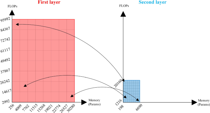
An \(8\times 8\) grid corresponding to the LeNet5 model. Two FC layers have been selected for factorization. The left part of the figure depicts the first layer with shape \(400\times 120\) (48,120 parameters) and the right part shows the second layer with shape \(120\times 84\) (10,164 parameters). For each grid tile in the first layer, there is a corresponding unique grid tile cell in the second layer

4 Experimental Results
Our evaluation is based on seven DNN models: LeNet5 (on MNIST and Fashion-MNIST datasets), LeNet300 (on MNIST dataset), AlexNet (on CIFAR10 and CIFAR100 datasets), VGG16 (on CIFAR10 and CIFAR100 datasets), VGG19 (on CIFAR10 and CIFAR100 datasets), VoxNet (on ModelNet10 and ModelNet40 datasets); and a Clock Detection (CD) model (trained with self-generated dataset). In all cases, we compare our experimental results to the baseline (non-factorized) model. All experiments are initialized from reference models trained for 100 epochs. For each compressed model, the obtained validation accuracy, the model size (number of parameters), and FLOPs are reported. The calculation of FLOPs is based on the assumption that each multiplication or addition is considered as one FLOP. For example, in a forward pass through a FC layer with a weight matrix of \(m\times n\) and a bias of \(n\times 1\), the considered FLOPs are \(2\times m\times n\). Finally, an \(8\times 8\) grid is used in all the cases following the log (memory)/linear (FLOPs) tiling strategy.

3D graphs showcasing the final sets of solutions for the MMMS strategy
The obtained results for the MMMS strategy are shown in Fig. 10 as 3D graphs (memory, FLOPs, and accuracy) for each studied model and dataset. In each graph in Fig. 10, the green circles correspond to the non-factorized model, the blue circles to the extracted solutions with accuracy drop less than 1% with respect to the initial model, and the red triangles to the solutions with accuracy drop more than 1%. In addition, the solution with the lowest memory footprint in each case is annotated with the black arrow.
As it is evident from Fig. 10, the proposed methodology is able to extract a set of solutions with a maximum accuracy drop of less than 1% in all cases. In particular, the number of blue circles ranges from 100 in LeNet300 model on MNIST dataset (Fig. 10c) to 196 in LeNet5 model on MNIST dataset (Fig. 10a). On average, the number of solutions annotated with the blue circles is 144 across all studied models. Moreover, among the latter set of extracted solutions, the majority of them exhibit a significant reduction in memory and FLOPs requirements. For example, the gathered results on CIFAR10 dataset show that our approach achieves a 99.7% memory reduction in the VGG16 and VGG19 models (Fig. 10d and f respectively) and 93.9% memory reduction in AlexNet model (Fig. 10h). Most significantly, this memory-FLOPs reductions are combined with an increase in the prediction accuracy (1.4%, 0.19%, and 1.4%, respectively). Similar results can be seen in the other studied models as well.
To further analyze the characteristics of the output solutions, Table 2 depicts three specific example cases for all the models considered in this work assuming that the MMMS mapping strategy is employed. The three cases correspond to the solutions with: highest reported accuracy (HA), lowest memory (LM), and lowest FLOPs (LF). When two datasets have been used for a specific model, the corresponding table entry shows the results for both datasets.
As Table 2 indicates, our methodology is able to extract LRF solutions exhibiting a reduction in memory footprint from 35.2% (in AlexNet) up to 99.8% (in VoxNet) and a reduction in the number of FLOPs from 5.7% (in AlexNet) up to 92.3% (in AlexNet). If we concentrate in the HA cases, in six out of seven studied models, a noticeable increase in model accuracy is observed (from 0.02% up to 5.3%). The only exception is the LeNet300 model in which an meager accuracy drop of 0.25% is reported. However, even in this case, the HA solution is associated with a 58.1% and 37.1% reduction in memory and FLOPs requirements, respectively.
Finally, Fig. 11 compares the two main tile mapping strategies proposed in this work. While all results presented so far refer to the (baseline) MMMS strategy, Fig. 11 showcases the additive benefits when the eN2CMS mapping strategy is employed. As mentioned, the last step in our methodology is to go through the derived solutions and apply specific high-level criteria. These criteria can enforce targeted constrains in terms of memory footprint reduction, and/or FLOPs reduction, and/or accuracy loss enforsed either by the user or the application. While different high level constrains can be applied, the statistics depicted in Fig. 11 assume two different scenarios: 75_75_1.5 (dark blue bar segments) means that the output solutions should exhibit at least 75% memory and FLOPs reduction, and maximum 1.5% accuracy drop compared to the initial model. Similarly, 50_50_1.5 (light blue bar segments) implies at least 50% memory and FLOPs reduction, and maximum 1.5% accuracy drop. The results in Fig. 11 are presented as stacked bars and show the absolute number of extracted solutions for each studied model and associated dataset.

Output solutions (absolute numbers) for the MMMS and eN2CMS strategies based on two different sets of high level criteria. The X_Y_Z notation means at least X% memory reduction, Y% FLOPs reduction, and maximum Z% accuracy drop
As it is evident from Fig. 11, the eN2CMS strategy manages to significantly increase the number of solutions with both criteria. However, this comes with a cost: more solutions should go through the re-evaluation (calibration) phase. On the other hand, the MMMS strategy is always able to identify and output solutions in both cases (employed criteria) although the number of solutions is lower. For example, in VGG16 on CIFAR100, the MMMS strategy elicits five solutions, while 13 solutions are derived by eN2CMS when the 75_75_1.5 case is used. The difference between the two strategies becomes more pronounced in the 50_50_1.5 case: 30 solutions in MMMS and 68 solutions in eN2CMS for VGG16 model on CIFAR10 dataset. In any case, both strategies exhibits different trade-offs in terms of quality of extracted solutions (in terms of memory, FLOPs, and accuracy) versus time needed for the re-evaluation/calibration phases. Further analysing this behavior by formulating more targeted tiling and mapping strategies is part of our future work.
5 Conclusions and Future Work
This paper presents a practical methodology that formulates the compression problem in DNN models using LRF as a DSE problem. The proposed methodology is able to extract a suitable set of LFR configurations in a reasonable time. Our experimental findings using seven different DNN models reveal that the proposed approach can offer a wide range of solutions that are able to compress the input DNN models up to 99.8% with minimal impact in prediction accuracy.
In our future work, we are planning to investigate additional techniques to further prune the design space. Furthermore, we also plan to extent and customize our methodology to NN models belonging to different application areas, such as object detection, image segmentation, and text and video processing.
References
Hussain, F., Hussain, R., Hassan, S.A., Hossain, E.: Machine learning in IoT security: current solutions and future challenges. IEEE Commun. Surv. Tutor. 22(3), 1686–1721 (2020). https://doi.org/10.1109/COMST.2020.2986444
Saraswat, S., Gupta, H.P., Dutta, T.: A writing activities monitoring system for preschoolers using a layered computing infrastructure. IEEE Sens. J. 20, 3871–3878 (2020). https://doi.org/10.1109/JSEN.2019.2960701
Mishra, A., Latorre, J.A., Pool, J., Stosic, D., Stosic, D., Venkatesh, G., Yu, C., Micikevicius, P.: Accelerating sparse deep neural networks. arXiv:2104.08378 (2021)
Akmandor, A.O., YIN, H., Jha, N.K.: Smart, secure, yet energy-efficient, internet-of-things sensors. IEEE Trans. Multi-Scale Comput. Syst. 4, 914–930 (2018). https://doi.org/10.1109/TMSCS.2018.2864297
Long, X., Ben, Z., Liu, Y.: A survey of related research on compression and acceleration of deep neural networks. J. Phys. Conf. Ser. 1213, 052003 (2019). https://doi.org/10.1088/1742-6596/1213/5/052003
Cheng, Y., Wang, D., Zhou, P., Zhang, T.: A survey of model compression and acceleration for deep neural networks. arXiv:1710.09282 (2017)
Pasandi, M.M., Hajabdollahi, M., Karimi, N., Samavi, S.: Modeling of pruning techniques for deep neural networks simplification. arXiv:2001.04062 (2020)
Song, Z., Fu, B., Wu, F., Jiang, Z., Jiang, L., Jing, N., Liang, X.: DRQ: dynamic region-based quantization for deep neural network acceleration. In: ACM/IEEE 47th Annual International Symposium on Computer Architecture (ISCA), 29 May–3 June 2020 (2020)
Huang, F., Zhang, L., Yang, Y., Zhou, X.: Probability weighted compact feature for domain adaptive retrieval. In: Proceedings of the IEEE/CVF Conference on Computer Vision and Pattern Recognition (CVPR), 14–19 June 2020 (2020)
Blakeney, C., Li, X., Yan, Y., Zong, Z.: Parallel Blockwise knowledge distillation for deep neural network compression. IEEE Trans. Parallel Distrib. Syst. 32, 1765–1776 (2021). https://doi.org/10.1109/TPDS.2020.3047003
Phan, A.-H., Sobolev, K., Sozykin, K., Ermilov, D., Gusak, J., Tichavskỳ, P., Glukhov, V., Oseledets, I., Cichocki, A.: Stable low-rank tensor decomposition for compression of convolutional neural network. In: European Conference on Computer Vision, 23–28 August 2020 (2020)
He, Y., Kang, G., Dong, X., Fu, Y., Yang, Y.: Soft filter pruning for accelerating deep convolutional neural networks. arXiv:1808.06866 (2018)
He, Y., Kang, G., Dong, X., Fu, Y., Yang, Y.: Channel pruning for accelerating very deep neural networks. In: Proceedings of the IEEE International Conference on Computer Vision (ICCV), 22–29 October 2017 (2017)
Han, S., Pool, J., Tran, J., Dally, W.: Learning both weights and connections for efficient neural network. In: Advances in Neural Information Processing Systems, 7–12 December 2017 (2015)
Gou, J., Yu, B., Maybank, S.J.: Knowledge distillation: a survey. Int. J. Comput. Vis. 129, 1789–1819 (2021). https://doi.org/10.1007/s11263-021-01453-z
Novikov, A., Izmailov, P., Khrulkov, V., Figurnov, M., Oseledets, I.V.: Tensor train decomposition on tensorflow (t3f). J. Mach. Learn. Res. 21(30), 1–7 (2020)
Abadi, M., Barham, P., Chen, J., Chen, Z., Davis, A., Dean, J., Devin, M., Ghemawat, S., Irving, G., Isard, M., others.: TensorFlow: a system for Large-Scale machine learning. In: 12th USENIX Symposium on Operating Systems Design and Implementation (OSDI 16), 2–4 November 2016 (2016)
Kokhazadeh, M., Keramidas, G., Kelefouras, V., Stamoulis, I.: A Design space exploration methodology for enabling tensor train decomposition in edge devices. In: International Conference on Embedded Computer Systems: Architectures, Modeling, and Simulation (SAMOS XXII), 3–7 July 2022 (2022)
Sainath, T.N., Kingsbury, B., Sindhwani, V., Arisoy, E., Ramabhadran, B.: Low-rank matrix factorization for deep neural network training with high-dimensional output targets. In: IEEE International Conference on Acoustics, Speech and Signal Processing, 26–31 May 2013 (2013)
Zhang, J., Lei, Q., Dhillon, I.: Stabilizing gradients for deep neural networks via efficient SVD parameterization. In: Proceedings of the 35th International Conference on Machine Learning, 10–15 Jul 2018 (2018)
Bejani, M.M., Ghatee, M.: Theory of adaptive SVD regularization for deep neural networks. Neural Netw. 128, 33–46 (2020). https://doi.org/10.1016/j.neunet.2020.04.021
Swaminathan, S., Garg, D., Kannan, R., Andres, F.: Sparse low rank factorization for deep neural network compression. Neurocomputing 398, 185–196 (2020). https://doi.org/10.1016/j.neucom.2020.02.035
Chorti, A., Picard, D.: Rate analysis and deep neural network detectors for SEFDM FTN systems. arXiv:2103.02306 (2021)
Ganev, I., van Laarhoven, T., Walters, R.: Universal approximation and model compression for radial neural networks. arXiv:2107.02550 (2021)
Chee, J., Renz, M., Damle, A., De Sa, C.: Pruning neural networks with interpolative decompositions. arXiv:2108.00065 (2021)
Chan, T.K., Chin, C.S., Li, Y.: Non-negative matrix factorization-convolutional neural network (NMF-CNN) for sound event detection. arXiv:2001.07874 (2020)
Li, D., Wang, X., Kong, D.: Deeprebirth: Accelerating deep neural network execution on mobile devices. In: Proceedings of the AAAI Conference on Artificial Intelligence, 2–7 February 2018 (2018)
Bai, Z., Li, Y., Woźniak, M., Zhou, M., Li, D.: Decomvqanet: decomposing visual question answering deep network via tensor decomposition and regression. Pattern Recognit. 110, 107538 (2021). https://doi.org/10.1016/j.patcog.2020.107538
Frusque, G., Michau, G., Fink, O.: Canonical Polyadic Decomposition and Deep Learning for Machine Fault Detection. arXiv:2107.09519 (2021)
Ma, R., Lou, J., Li, P., Gao, J.: Reconstruction of generative adversarial networks in cross modal image generation with canonical polyadic decomposition. Wireless Commun. Mobile Comput. 2021, 1747–1756 (2021). https://doi.org/10.1016/j.patcog.2020.107538
Kolda, T.G., Bader, B.W.: Tensor decompositions and applications. SIAM Rev. 51, 455–500 (2009). https://doi.org/10.1137/07070111X
Idelbayev, Y., Carreira-Perpinan, M.A.: Low-rank compression of neural nets: learning the rank of each layer. In: Proceedings of the IEEE/CVF Conference on Computer Vision and Pattern Recognition, 14–19 June 2020 (2020)
Oseledets, I.V.: Tensor-train decomposition. SIAM J. Sci. Comput. 33, 2295–2317 (2011). https://doi.org/10.1137/090752286
Novikov, A., Podoprikhin, D., Osokin, A., Vetrov, D.P.: Tensorizing neural networks. In: Advances in Neural Information Processing Systems, Vol. 28 (2015)
Pollock, D.S.G.: Multidimensional arrays, indices and Kronecker products. Econometrics 9, 18–33 (2021). https://doi.org/10.3390/econometrics9020018
Golub, G.H., Van Loan, C.F.: Matrix Computations. JHU Press, Baltimore (2013)
Hawkins, C., Liu, X., Zhang, Z.: Towards compact neural networks via end-to-end training: A Bayesian tensor approach with automatic rank determination. SIAM J. Math. Data Sci. 4, 46–71 (2022). https://doi.org/10.1137/21M1391444
Cheng, Z., Li, B., Fan, Y., Bao, Y.: A novel rank selection scheme in tensor ring decomposition based on reinforcement learning for deep neural networks. In: IEEE International Conference on Acoustics, Speech and Signal Processing (ICASSP), 4–8 May 2020 (2020)
Kim, T., Lee, J., Choe, Y.: Bayesian optimization-based global optimal rank selection for compression of convolutional neural networks. IEEE Access 8, 17605–17618 (2020). https://doi.org/10.1109/ACCESS.2020.2968357
LeCun, Y., others.: Lenet-5, convolutional neural networks. 20(5), 14 (2015). http://yann.lecun.com/exdb/lenet
Krizhevsky, A., Sutskever, I., Hinton, G.E.: Imagenet classification with deep convolutional neural networks. In: Advances in neural information processing systems, vol. 25 (2012)
Acknowledgements
The authors would like to thank anonymous reviewers of the SAMOS XXII conference for their valuable remarks on the content of the paper.
Funding
Open access funding provided by HEAL-Link Greece. This research has been supported by the H2020 Framework Program of the European Union through the Affordable5G Project (Grant Agreement 957317) and by a sponsored research agreement between Applied Materials, Inc. and Aristotle University of Thessaloniki, Greece (Grant Agreement 72714).
Author information
Authors and Affiliations
Contributions
The authors confirm contribution to the paper as follows: study conception and design: MK, GK, VK, and IS; data collection: MK; analysis and interpretation of results: MK, GK, and VK; draft manuscript preparation: MK, GK, and VK. All authors reviewed the results and approved the final version of the manuscript.
Corresponding authors
Ethics declarations
Conflicts of interest
All authors declare that they have no conflicts of interest.
Additional information
Publisher's Note
Springer Nature remains neutral with regard to jurisdictional claims in published maps and institutional affiliations.
Rights and permissions
Open Access This article is licensed under a Creative Commons Attribution 4.0 International License, which permits use, sharing, adaptation, distribution and reproduction in any medium or format, as long as you give appropriate credit to the original author(s) and the source, provide a link to the Creative Commons licence, and indicate if changes were made. The images or other third party material in this article are included in the article's Creative Commons licence, unless indicated otherwise in a credit line to the material. If material is not included in the article's Creative Commons licence and your intended use is not permitted by statutory regulation or exceeds the permitted use, you will need to obtain permission directly from the copyright holder. To view a copy of this licence, visit http://creativecommons.org/licenses/by/4.0/.
About this article

Cite this article
Kokhazadeh, M., Keramidas, G., Kelefouras, V. et al. A Practical Approach for Employing Tensor Train Decomposition in Edge Devices. Int J Parallel Prog 52, 20–39 (2024). https://doi.org/10.1007/s10766-024-00762-3
Received:
Accepted:
Published:
Issue Date:
DOI: https://doi.org/10.1007/s10766-024-00762-3