Analyzing Size of Loss Frequency Distribution Patterns: Uncovering the Impact of the COVID-19 Pandemic

Abstract

This study delves into a critical examination of the Size of Loss distribution patterns in the context of auto insurance during pre- and post-pandemics, emphasizing their profound influence on insurance pricing and regulatory frameworks. Through a comprehensive analysis of the historical Size of Loss data, insurers and regulators gain essential insights into the probabilities and magnitudes of insurance claims, informing the determination of precise insurance premiums and the management of case reserving. This approach aids in fostering fair competition, ensuring equitable premium rates, and preventing discriminatory pricing practices, thereby promoting a balanced insurance landscape. The research further investigates the impact of the COVID-19 pandemic on these Size of Loss patterns, given the substantial shifts in driving behaviours and risk landscapes. Also, the research contributes to the literature by addressing the need for more studies focusing on the implications of the COVID-19 pandemic on pre- and post-pandemic auto insurance loss patterns, thus offering a holistic perspective encompassing both insurance pricing and regulatory dimensions.

1. Introduction

The study of Size of Loss distributions in auto insurance is essential for insurance pricing, and it also has significant implications for auto insurance rate regulation (Lee et al. 2022; Mohamed 2022). Insurance companies and regulators can effectively evaluate the risks linked to specific groups of claim amounts by looking into the historical Size of Loss distributions across different coverages or territories. This analysis aids in estimating both the probabilities and magnitudes of incurred claims so that the overall premium level can be better determined. Moreover, insurers utilize this historical data to ascertain suitable premiums for reinsurance contracts (Kelly et al. 2020; Mert and Selcuk-Kestel 2021) by further looking into the large loss distribution based on the Size of Loss distribution. These insurance contracts are often called stop-loss insurance (Denuit and Robert 2021). A profound comprehension of the Size of Loss empowers insurers to make well-informed decisions regarding the acceptance or rejection of reinsurance contracts and the establishment of suitable terms and conditions for coverage. Moreover, as insurance companies must allocate funds to cover possible claims and incurred losses that have yet to be paid, a comprehensive study of the Size of Loss distribution enables them to efficiently manage case reserves, ensuring the availability of adequate funds for claim payouts in the future. Understanding typical loss sizes helps establish appropriate reserve levels, which are often determined via modern machine learning approaches (Blier-Wong et al. 2020; De Felice and Moriconi 2019).

Shifting the attention away from examining the impact of the Size of Loss distribution on insurance pricing, it is crucial to uncover the underlying patterns within the Size of Loss distribution for different major coverages, regions and across different accident years. This critical focus is important for auto insurance regulators as they evaluate and authorize rate changes in the auto insurance sector. It ensures insurers apply precise and equitable premium rates, avoiding excessive charges. The study of the Size of Loss data empowers regulators to foster healthy competition and pre-empt market disruptions that might otherwise have adverse effects on policyholders. In this aspect, regulators need to study the historical Size of Loss data to evaluate the normal level loss distribution and large loss distributions. By considering the Size of Loss patterns, regulators can ensure that insurance rates remain fair and accurately reflect the risk associated with different insurance coverages or presented by various groups of drivers from other territories. This practice actively combats discriminatory pricing strategies, promoting equitable insurance for all drivers (Kelly and Kleffner 2003) and making insurance regulation more effective (Li et al. 2010).

Investigating the impact of the COVID-19 pandemic on auto insurance loss patterns is important as it has led to significant shifts in driving behaviours, which may lead to completely different loss patterns before and after the COVID-19 pandemic (Dong et al. 2022; Katrakazas et al. 2020; Stavrinos et al. 2020). By comprehensively understanding these changes, insurers can adjust their risk assessments and future policies to accurately reflect the new norms and behaviours exhibited by drivers both during and after the pandemic. With the considerable changes in travel patterns and work-from-home arrangements, the risk landscape for auto insurance has fundamentally transformed. This necessitates a thorough investigation of the COVID-19 pandemic impact on the Size of Loss patterns, enabling insurers to evaluate the revised risk levels associated with driving during and post-pandemic (Ciuffini et al. 2023). Based on this evaluation, insurers can then make informed decisions regarding premium adjustments for policyholders.

Furthermore, the impact of the COVID-19 pandemic on auto insurance loss patterns calls for necessary adjustments in underwriting practices. Insurers must consider various factors, including changes in commuting distances, usage frequency, and the types of road users during the pandemic (Gupta et al. 2021; Katrakazas et al. 2021; Sutherland et al. 2020) to refine their underwriting processes accurately. This understanding of the evolving risk profiles of drivers and vehicles is imperative for maintaining the financial sustainability of insurance companies. With precise insights into the shifting risk landscape, insurers can effectively manage their case reserves and pricing strategies, thereby ensuring their financial stability and ability to provide coverages and pay out claims as required.

Understanding the pandemic’s impact on auto insurance loss patterns also empowers insurance companies to tailor their policies to meet the evolving needs of their policyholders. By grasping the changes in risk exposure, insurers can develop more pertinent and responsive insurance products and services that effectively address the current and future demands of policyholders. Thoroughly investigating the COVID-19 pandemic’s impact on auto insurance loss patterns thus equips insurers to make informed decisions, adapt their strategies, and secure the long-term sustainability of their operations amidst changing circumstances.

In this research, we developed statistical models using the Size of Loss data corresponding to different accident years, aiming to assess the impact of the COVID-19 pandemic. These statistical models were constructed based on different coverages, regions (Urban and Rural), and statistical territories. This consideration arose from the observation that auto insurance loss patterns often exhibit distinct variations across different coverages and regions. The novelty of this study lies in its examination of the COVID-19 impact from both insurance pricing and regulation perspectives, a facet that has yet to be explored in existing literature focusing on pre- and post-pandemic loss patterns.

The remainder of the paper is organized as follows: Section 2 reviews the current state of the art, drawing parallels to our study. In Section 3, we delve into the data used, statistical models employed to analyze the Size of Loss data. Section 4 presents the findings and analysis. Finally, Section 6 reports the key findings and offers concluding remarks.

2. Literature Review

The COVID-19 pandemic has had far-reaching consequences, affecting various aspects of society, including finance, risk management, insurance and economic modelling. This literature review provides an overview of recent research papers that shed light on the impact of COVID-19 on these domains. Particularly, we focus on the study of the impact of COVID-19 on financial market dynamics. This aspect of literature analysis is related to loss distributions and helps us better understand the direct and indirect influence on auto insurance pricing and market dynamics. Azimli (2020) investigates how COVID-19 has affected the dependence and structure of the risk-return relationship in US financial markets using quantile regression. The results indicate a left-tailed asymmetric dependence structure of sectoral returns with a market portfolio. That is, increased investor attention towards coronavirus, measured as GSIC (Google Search Index for Coronavirus), has negative and higher effects on industries in the lower tail of distribution but positive and lower effects on industries in the upper tail of distribution. This observation is similar to the effect of COVID-19 on the Size of Loss distributions by major coverage, which impacted the lower tails distribution more. Ji et al. (2020) examine the impact of a safe-haven asset in a simple mean-variance portfolio and whether it can be used to offset a tail change in the equity index during the COVID-19 pandemic. In particular, they introduce a sequential monitoring procedure to detect changes in the left-quantiles of asset returns. Again, studying the tail behaviour of return distribution and its COVID-19 pandemic effect could provide insights into how the insurance investment portfolio should satisfy the requirement of return on equality in auto insurance rate regulation.

The reliability and accuracy of the case reserving in auto insurance depends on the investment outcomes in both domestic and international financial markets. The dynamics of major financial indexes provide an overall big picture of how they are related, particularly for periods before and during the COVID-19 pandemic. Ghorbe et al. (2022) analyzes the risk spillover between China and G7 stock markets before and during COVID-19 pandemic. They found that downside and upside risk spillovers were significantly larger before the COVID-19 pandemic in all cases except between CAC 40/DAX and S&P/SSE pairs. They also find a significant and asymmetrical two-way risk transmission between the majority of pair markets. The degree of asymmetry is highly sensitive to the choice of the entire cumulative distributions or distribution tails. The study of the financial market dynamics can go from traditional financial indexes to cryptocurrency markets, which are much more volatile. Such a study is also crucial when addressing market uncertainty during the COVID-19 crisis. The techniques or focuses used to uncover the financial dynamics may include extreme value regressions or tail distributions, or others. Thazhungal (2022) delves into the application of extreme value theory to cryptocurrency markets in the context of COVID-19. In particular, it finds that after including the technical trading indicators as control variables in the extreme value regressions, the predictive power significantly improved during the COVID-19 crisis. This may indicate the market dynamics are heavily affected by a major global health crisis. Nehrebecka (2023) tracks the evolution of tail risk in banks’ non-performing loan portfolios before and during the COVID-19 pandemic and evaluates the impact of sector concentration risk on economic capital. Using a multi-factor structural model, the study identifies increased tail risk during 2015–2017, followed by a decline. As auto insurance reserving highly depends on investment returns, insurance companies may have to consider this when investing their income from insurance premiums. These studies contribute to a more nuanced understanding of the factors influencing investment returns in the auto insurance industry amid the COVID-19 pandemic. By considering the sectoral impacts, identifying safe-haven assets, managing global risk spillover, diversifying across asset classes, and assessing tail risk in financial institutions, insurers can make more informed investment decisions to optimize returns in a challenging economic environment.

The insurance loss pattern may be significantly changed due to the changes in claim frequency and severity, and various research work has been devoted to the study of the COVID-19 pandemic’s impact on insurance losses. This impact caused by the COVID-19 pandemic may further affect the changes in the insurance underwriting process. Qiu (2020) examines the insured losses incurred due to COVID-19 and their impact on the insurance industry. It further assesses the current modelling capabilities for pandemic risk and how the insurance industry utilizes these models. The paper recommends enhancing these models in the future and leveraging them for effective pandemic risk insurance, which may provide insights into the effect on auto insurance due to future global health crises. Also, the risk associated with the pandemic may lead to new types of insurance, and the study of the insurability of pandemic risk becomes fundamental. Richter and Wilson (2020) examines how the insurability of pandemic risk can be improved by establishing resilience upfront and planning contingency actions for crisis scenarios if underwriting policies and scenario analysis are appropriately employed. They conclude that business interruption is not an insurable risk if it is caused by containment activities to manage a global pandemic, and insurers need to improve policy wording, focusing on increased harmonization, transparency, and enforceability. On the other hand, it is highly desirable to have consistency between insurance price and the underlying loss distribution. This means that accurate pricing can be done only when the characteristics of loss distribution are properly captured. Grundl et al. (2021) delves into the private market’s capacity for pandemic insurance, introducing a theoretical framework that explicates how the equilibrium price of pandemic insurance is influenced by accumulation risk, covariance with other claims, and covariance with stock market performance. They estimate the relationship between insurance price markup and the tail characteristics of loss distribution using the natural catastrophe (NatCat) insurance market data. It shows the process of calibrating the loss distribution of a hypothetical insurance contract designed to mitigate the pandemic’s impact on small businesses.

3. Materials and Methods

3.1. Data

This research focuses on analyzing regulatory Size of Loss data sourced from the General Insurance Statistical Agency of Canada, which can be accessed at the following URL: https://www.gisa.ca (accessed on 3 July 2023). To initiate our investigation, the first crucial step involves data preprocessing, ensuring the data is sanitized, uniform, and prepared for comprehensive analysis. The main objective is to consolidate claim counts and loss amounts, taking into account various factors, including rural-urban indicators, statistical territories, accident years, and major coverage types, including Accident Benefit (AB), Third Part Liability (TPL), and Collision (CL). AB, CL, and TPL coverages are integral components of auto insurance, each serving a specific purpose in providing financial protection to policyholders and third parties involved in car accidents. Analyzing regulatory insurance claims data separated by coverage types is essential for insurers to effectively manage risks, underwrite policies accurately, set appropriate pricing, and develop innovative insurance solutions that meet the evolving needs of their customers.

One particular characteristic of the Size of Loss data is the irregular length of the interval. Since the Size of Loss distribution is a grouped frequency distribution, and the theoretical range of claim amount is zero to ∞, it is practically necessary to have an increasing interval length with a dramatic change at the right tail. To evaluate the COVID-19 pandemic effect, we undertake a comparative study of the Size of Loss distributions before and during the pandemic. The years 2017, 2018, and 2019 represent the pre-pandemic period, while the subsequent years will signify the period during the pandemic. This comparative analysis through a predictive modelling using Generalize Linear Models (GLM) seeks to identify any significant alterations or trends in the Size of Loss distributions, particularly in response to the unprecedented events brought about by the pandemic.

3.2. Generalized Linear Model

GLM is a statistical modeling technique employed to investigate relationships between a dependent variable and one or more independent variables. This approach enhances the flexibility of linear regression by allowing the modeling of a wide range of data distributions, surpassing the limitations associated with the conventional normal distribution. The main elements of a GLM are as follows:

• Link function: GLMs integrate a link function that establishes a connection between the linear predictor (a weighted sum of the independent variables) and the mean of the dependent variable. This link function aims to capture the mathematical relationship between the response variable and predictors and it can be a linear or non-linear function. Often the canonical link function is chosen based on the distribution of the response variable and is defined such that it relates the linear predictor to the mean of the response variable in a natural way according to that distribution. Choosing the canonical link ensures that the GLM estimation procedure is efficient and that the resulting model is mathematically well-defined. The canonical link function for a Gaussian distribution is the identity function, the logarithmic function is the canonical link or a Poisson distribution, and the logit function is for a binomial distribution.
• Error distribution: GLMs have the capacity to model a broad spectrum of probability distributions for the response variable, such as Gaussian (normal), Poisson, binomial, gamma, and others. The selection of the distribution relies on the characteristics of the data and its variability.
• Linear predictor: The linear predictor of a GLM combines independent variables using their respective coefficients. The link function transforms this linear combination to ensure that the predicted values align with the appropriate scale for the chosen distribution.

GLMs employ deviance as a metric to assess the model’s alignment with the data. Deviance serves as a measure of the difference between observed data and model predictions, where lower values signify a superior model fitting. The estimation of model parameters can be accomplished through diverse techniques, including Maximum Likelihood Estimation (MLE) or Iteratively Reweighted Least Squares (IRLS), depending on the selected error distribution. Employing the GLM model in this study offers the advantage of capturing the linear effects induced by each level of the predictor, facilitating the interpretation of the model’s results.

GLM stands out as a good choice for investigating the impact of the COVID-19 pandemic on the Size of Loss distribution of auto insurance due to its versatile nature. Offering flexibility in error probability distribution, GLMs can accommodate a wide range of response variable types. This adaptability is crucial when exploring the diverse outcomes associated with events. The incorporation of a link function enables the modelling of relationships between explanatory variables and the response, allowing for a nuanced representation of the event’s impact. Moreover, the capacity to capture non-linear relationships is valuable when dealing with complex insurance system dynamics. The model’s ability to incorporate categorical predictors is essential when characterizing events with categorical factors. Statistical inference within the GLM framework supports the assessment of event significance and parameter estimation uncertainty. Additionally, the interpretability of GLM facilitates a clear understanding of how specific events influence the system, making it a powerful tool for drawing meaningful conclusions and informing decisions across various domains, including complex insurance systems.

3.3. Predictive Modelling of Size of Loss Distributions

In our modelling phase, using GLM, we explore how claim frequency is affected by the Size of Loss interval and other factors, including different accident years that will reflect the COVID-19 pandemic effect. The choice of error distribution family and link function is crucial and depends on the nature of the response variable and the research objectives. To model the claim counts, which is a numerical variable representing the number of claims, we considered two different GLM configurations:

• Gaussian distribution with identity link function: We opted for the Gaussian distribution with identity link function when modelling the data. This combination assumes that the response variable follows a normal distribution, making it suitable for modelling continuous numerical variables. In this case, we used it to capture some models where the distribution of the response variable resembled a normal distribution.
• Poisson distribution with log link function: We have used the Poisson distribution with a log link function. The choice of Poisson distribution is particularly appropriate when dealing with count data, such as the number of claims. The Poisson distribution is well suited to modelling rare events whose variance is roughly equal to the mean. The logarithmic link function ensures that predicted values remain non-negative, essential in the context of count data. Using the Poisson distribution as the error distribution in GLMs offers a flexible and interpretable framework for modeling count data, with implications for the ease of interpretation of coefficients.

However, after the comparative study, the Gaussian distribution has been selected as the primary modeling framework for characterizing the variability in claim frequencies within each interval (i.e., Size of Loss) across various accident years. This choice is rooted in its capacity to yield results that are readily interpretable, thereby facilitating a clearer understanding of the obtained insights. Moreover, given the repeated nature of the data, with multiple measurements taken over time, the Gaussian distribution emerges as a particularly fitting choice. Utilizing the Gaussian distribution enables us to effectively capture the uncertainty inherent in observations spanning different major insurance coverages, geographical regions, and statistical territories. By leveraging this distribution, we aim to provide a robust framework for analyzing and interpreting the complexities of the data, thereby enhancing the reliability and validity of our findings. Unfortunately, the Poisson distribution with a log link does not lead to better results when compared with the Gaussian distribution case. This may be because Gaussian distribution is a natural choice for capturing the measurement errors as our data is the repeated measures across different accident years.

3.4. Modelling Claim Frequency by Region and Major Coverage

The following predictive model is proposed to model claim frequency of Size of Loss:

$$\begin{array}{c}\hfill TotalClaimCoun{t}_{kl}^{\left(ij\right)}={\gamma }_0^{\left(ij\right)}+{\gamma }_{1k}^{\left(ij\right)}\times SizeOfLossRang{e}_k^{\left(ij\right)}+{\gamma }_{2l}^{\left(ij\right)}\times AccidentYea{r}_l+{\epsilon }_{kl}^{\left(ij\right)},\end{array}$$

(1)

where, ${\gamma }_0^{\left(ij\right)}$ represents the model intercept, ${\gamma }_{1k}^{\left(ij\right)}$ captures the impact of the kth size of the loss range, and ${\gamma }_{2l}^{\left(ij\right)}$ accounts for the effect of the lth accident year. The superscript $ij$ indicates ith region and jth coverage. There are two regions: Urban and Rural, and three major coverages: AB, CL, and TPL. The error term ${\epsilon }_{kl}^{\left(ij\right)}$ represents the unexplained variability associated with the model for the ith region and jth major coverage. These models allowed us to quantify the relationships between the predictor variables, $SizeOfLossRange$ and $AccidentYear,$ and the response variable, $TotalClaimCount$. The $SizeOfLossRange$ consists of a set of irregular, consecutive intervals, and for the ease of presenting these intervals, we only give the upper limit in the reported results. For instance, Upper Limit 2000 denotes interval [1000, 2000), and Upper Limit 2,000,000 in the reported results means interval [1,000,000, 2,000,000). The resulting coefficients provide insights into the magnitude and direction of these relationships, shedding light on how changes in these predictors are associated with changes in claim counts.

3.5. Model with COVID-19 Indicator

In Model (1), the covariate $AccidentYear$ serves to estimate the effects attributed to various accident years. This estimation helps discern the impact of the COVID-19 pandemic, specifically in relation to the accident years 2020 and 2021. Nonetheless, the use of Model (1) for estimation entails the consideration of combined effects stemming from both the accident year and the influence of COVID-19. Consequently, we redefine the levels of $AccidentYear$ in an effort to potentially mitigate the influence stemming from the accident year itself. We transform the covariate $AccidentYear$ into $covidindicator$. Below are two strategies we employ to tackle this issue by restructuring the accident years.

• COVID-19 Single Level Effect:

  –

  Each of the accident years 2017, 2018, and 2019 is assigned a COVID indicator of 0.

  –

  Each of the accident years 2020 and 2021 is assigned a COVID indicator of 1.

• COVID-19 Two Levels Effect:

  –

  Each of the accident years 2017, 2018, and 2019 is assigned a COVID indicator of 0.

  –

  The accident year 2020 is assigned a COVID indicator of 1.

  –

  The accident year 2021 is assigned a COVID indicator of 2.

The covariate $AccidentYear$ in Model (1) is replaced by $covidindicator$, and the new equation is re-written with new coefficient parameters, which is given as follows

$$\begin{array}{c}\hfill TotalClaimCoun{t}_{kl}^{\left(ij\right)}={\alpha }_0^{\left(ij\right)}+{\alpha }_{1k}^{\left(ij\right)}\times SizeOfLossRang{e}_k^{\left(ij\right)}+{\alpha }_{2l}^{\left(ij\right)}\times covidindicato{r}_l+{\epsilon }_{kl}^{\left(ij\right)},\end{array}$$

(2)

3.6. Model with Statistical Territory and Major Coverage

In Ontario of Canada, the concept of ’statistical territories’ holds significant importance within the insurance industry, particularly for the assessment of auto insurance pricing and risk evaluation performed by auto insurance regulators. These territories represent defined geographical areas within the province, utilized by insurance companies to effectively calculate insurance premiums. The demarcation of these territories relies on multiple factors, including fundamental infrastructures, traffic patterns, population density, and other pertinent statistics. Insurance firms leverage statistical territories to evaluate the risks associated with insuring vehicles across different regions. Typically, areas with a history of higher accident rates, frequent thefts, or increased exposure to risk factors tend to warrant higher insurance premiums. Conversely, regions with lower risk profiles often attract comparatively lower premiums. In fact, the initial definitions of these statistical territories were not intended for insurance purposes; instead, their primary purpose is to assess the socio-economic status of the respective regions. However, these territories play a crucial role in the actuarial pricing to establish insurance rates for their policyholders. In this work, the introduction of statistical territories replaces the concept of ’region’ while maintaining the same model structure as Model (1).

4. Results

4.1. Results Based on Dot-Plots of Size of Loss

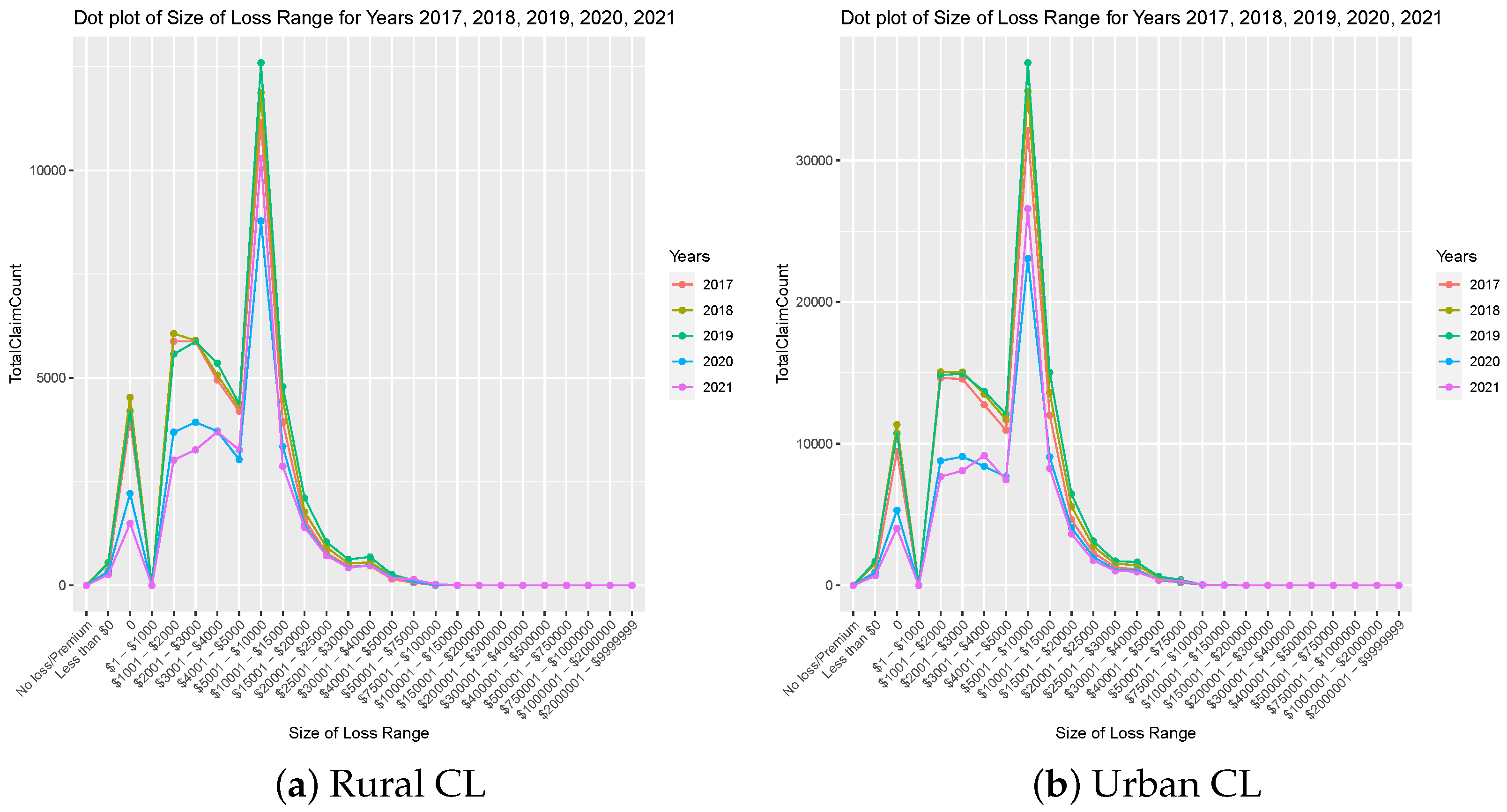
This section presents the findings obtained from the dot plots of the Size of Loss distribution, considering the aggregation of claim counts based on key factors such as rural-urban indicators, accident years, and main coverage types. Figure 1 displays the breakdown of the Size of Loss concerning the number of claim counts across the years 2017 to 2021, with a specific focus on distinguishing between rural and urban areas under AB coverage. Upon close examination, a distinct trend emerges, showing remarkable consistency in data from the pre-pandemic years (2017, 2018, and 2019). However, an observable shift becomes apparent in the years impacted by the COVID-19 pandemic (2020 and 2021), suggesting a notable influence of the pandemic on claim numbers. Similar observations are made for TPL coverage, as demonstrated in Figure 2, where a significant change in the pattern during 2020 and 2021 closely mirrors the trends observed in the context of AB coverage. Notably, this change is most pronounced in the claim size range of $1001 to $5000, possibly attributed to pandemic-induced shifts in driving behaviour, accident frequency, or other factors specific to liability claims within this range. The striking resemblance in the results for both CL (see Figure 3) and TPL coverage implies a shared response to external factors, reflecting their exposure to diverse risks. The parallel shift in patterns during 2020 and 2021, compared to earlier years, strongly indicates a pandemic-related effect, influenced by various factors such as the pandemic’s economic impact, changes in driving behaviour, potential delays in seeking medical care, and insurers’ adaptability to the evolving risk landscape. Thus, while claim counts associated with CL and TPL coverages may differ in specific accident years, their consistent response to the pandemic underscores the significant role of external events and changing circumstances in shaping insurance claims.

4.2. Results on Predictive Modelling of Size of Loss

Table 1. Model coefficients, sampling error of the estimates and goodness of fit measures for model with response associated with AB coverage, separated by Urban and Rural. Values are rounded to integers.

	Dependent Variable:
	TotalClaimCount (U)		TotalClaimCount (R)
	Normal	Poisson (Log Link)	Normal	Poisson (Log Link)
Upper Limit 2000	−9780 *** (1443)	−0 *** (0)	−3281 *** (387)	−1 *** (0)
Upper Limit 3000	−11,383 *** (1443)	−1 *** (0)	−4445 *** (387)	−1 *** (0)
Upper Limit 4000	−8953 *** (1443)	−0 *** (0)	−4435 *** (387)	−1 *** (0)
Upper Limit 5000	−19,138 *** (1443)	−1 *** (0)	−6138 *** (387)	−2 *** (0)
Upper Limit 10,000	−8215 *** (1443)	−0 *** (0)	−3906 *** (387)	−1 *** (0)
Upper Limit 15,000	−16,937 *** (1443)	−1 *** (0)	−5944 *** (387)	−1 *** (0)
Upper Limit 20,000	−18,941 *** (1443)	−1 *** (0)	−6276 *** (387)	−2 *** (0)
Upper Limit 25,000	−20,972 *** (1443)	−2 *** (0)	−6712 *** (387)	−2 *** (0)
Upper Limit 30,000	−22,183 *** (1443)	−2 *** (0)	−6993 *** (387)	−2 *** (0)
Upper Limit 40,000	−20,567 *** (1443)	−2 *** (0)	−6646 *** (387)	−2 *** (0)
Upper Limit 50,000	−22,456 *** (1443)	−2 *** (0)	−6976 *** (387)	−2 *** (0)
Upper Limit 75,000	−21,721 *** (1443)	−2 *** (0)	−6768 *** (387)	−2 *** (0)
Upper Limit 100,000	−24,146 *** (1443)	−3 *** (0)	−7289 *** (387)	−3 *** (0)
Upper Limit 150,000	−24,458 *** (1443)	−3 *** (0)	−7347 *** (387)	−3 *** (0)
Upper Limit 200,000	−25,343 *** (1443)	−4 *** (0)	−7585 *** (387)	−4 *** (0)
Upper Limit 300,000	−25,354 *** (1443)	−4 *** (0)	−7562 *** (387)	−4 *** (0)
Upper Limit 400,000	−25,606 *** (1443)	−4 *** (0)	−7664 *** (387)	−4 *** (0)
Upper Limit 500,000	−25,741 *** (1443)	−5 *** (0)	−7707 *** (387)	−5 *** (0)
Upper Limit 750,000	−25,726 *** (1443)	−5 *** (0)	−7702 *** (387)	−5 *** (0)
Upper Limit 1,000,000	−25,841 *** (1443)	−6 *** (0)	−7741 *** (387)	−5 *** (0)
Upper Limit 2,000,000	−25,806 *** (1443)	−5 *** (0)	−7727 *** (387)	−5 *** (0)
Upper Limit Inf	−25,916 *** (1443)	−8 *** (0)	−7773 *** (387)	−8 *** (0)
AccidentYear2018	105 (673)	0 *** (0)	42 (180)	0 *** (0)
AccidentYear2019	212 673)	0 *** (0)	8 (180)	0 (0)
AccidentYear2020	−2585 *** (673)	−0 *** (0)	−431 ** (180)	−0 *** (0)
AccidentYear2021	−2079 *** (673)	−0 *** (0)	−222 (180)	−0 *** (0)
Constant	26,791 *** (1105)	10 *** (0)	7896 *** (296)	9 *** (0)
Observations	115	115	115	115
Log Likelihood	−1038	−11,979	−887	−4125
Akaike Inf. Crit.	2130	24,012	1827	8305

Note: * $p<$ 0.1; ** $p<$ 0.05; *** $p<$ 0.01.

,

Table 2. Model coefficients, sampling error and goodness of fit measures for model with response associated with CL coverage, separated by Urban and Rural.

	Dependent Variable:
	TotalClaimCount (U)		TotalClaimCount (R)
	Normal	Poisson (Log Link)	Normal	Poisson (Log Link)
Upper Limit 2000	12,206 *** (1030)	25 (564)	4846 *** (320)	25 (935)
Upper Limit 3000	12,348 *** (1030)	25 (564)	4970 *** (320)	25 (935)
Upper Limit 4000	11,499 *** (1030)	25 (564)	4556 *** (320)	25 (935)
Upper Limit 5000	9970 *** (1030)	24 (564)	3832 *** (320)	25 (935)
Upper Limit 10,000	30,706 *** (1030)	26 (564)	10,937 *** (320)	26 (935)
Upper Limit 15,000	11,597 *** (1030)	25 (564)	3882 *** (320)	25 (935)
Upper Limit 20,000	4873 *** (1030)	24 (564)	1664 *** (320)	24 (935)
Upper Limit 25,000	2396 ** (1030)	23 (564)	839 ** (320)	23 (935)
Upper Limit 30,000	1336 (1030)	22 (564)	499 (320)	23 (935)
Upper Limit 40,000	1243 (1030)	22 (564)	538 * (320)	23 (935)
Upper Limit 50,000	458 (1030)	21 (564)	212 (320)	22 (935)
Upper Limit 75,000	302 (1030)	21 (564)	106 (320)	21 (935)
Upper Limit 100,000	48 (1030)	19 (564)	12 (320)	19 (935)
Upper Limit 150,000	20 (1030)	18 (564)	2 (320)	17 (935)
Upper Limit 200,000	3 (1030)	16 (564)	0 (320)	15 (935)
Upper Limit 300,000	3 (1030)	16 (564)	0 (320)	−0 (1322)
Upper Limit 400,000	0 (1030)	14 (564)	0 (320)	−0 (1322)
Upper Limit 500,000	0 (1030)	14 (564)	0 (320)	−0 (1322)
Upper Limit 750,000	0 (1030)	0 (798)	0 (320)	−0 (1322)
Upper Limit 1,000,000	0 (1030)	0 (798)	0 (320)	−0 (1322)
Upper Limit 2,000,000	0 (1030)	0 (798)	0 (320)	−0 (1322)
Upper Limit Inf	0 (1030)	0 (798)	0 (320)	−0 (1322)
AccidentYear2018	391 (480)	0 *** (0)	99 (149)	0 *** (0)
AccidentYear2019	631 (480)	0 *** (0)	169 (149)	0 *** (0)
AccidentYear2020	−1392 *** (480)	−0 *** (0)	−418 *** (149)	−0 *** (0)
AccidentYear2021	−1375 *** (480)	−0 *** (0)	−423 *** (149)	−0 *** (0)
Constant	349 (789)	−15 (564)	115 (245)	−16 (935)
Observations	115	115	115	115
Log Likelihood	−999	−1359	−865	−920
Akaike Inf. Crit.	2053	2773	1784	1893

Note: * $p<$ 0.1; ** $p<$ 0.05; *** $p<$ 0.01.

and

Table 3. Model coefficients, sampling error and goodness of fit measures for model with response associated with TPL coverage, separated by Urban and Rural.

	Dependent Variable:
	TotalClaimCount (U)		TotalClaimCount (R)
	Normal	Poisson (Log Link)	Normal	Poisson (Log Link)
Upper Limit 2000	46,611 *** (4057)	2 *** (0)	13,389 *** (991)	2 *** (0)
Upper Limit 3000	41,798 *** (4057)	2 *** (0)	12,801 *** (991)	2 *** (0)
Upper Limit 4000	33,905 *** (4057)	1 *** (0)	10,457 *** (991)	1 *** (0)
Upper Limit 5000	23,648 *** (4057)	1 *** (0)	6942 *** (991)	1 *** (0)
Upper Limit 10,000	84,365 *** (4057)	2 *** (0)	22,389 *** (991)	2 *** (0)
Upper Limit 15,000	20,537 *** (4057)	1 *** (0)	4844 *** (991)	1 *** (0)
Upper Limit 20,000	1681 (4057)	0 *** (0)	−6 (991)	−0 (0)
Upper Limit 25,000	−4694 (4057)	−1 *** (0)	−1559 (991)	−1 *** (0)
Upper Limit 30,000	−7296 * (4057)	−1 *** (0)	−2242 ** (991)	−1 *** (0)
Upper Limit 40,000	−5897 (4057)	−1 *** (0)	−1813 * (991)	−1 *** (0)
Upper Limit 50,000	−8302 ** (4057)	−1 *** (0)	−2531 ** (991)	−1 *** (0)
Upper Limit 75,000	−7981 * (4057)	−1 *** (0)	−2511 ** (991)	−1 *** (0)
Upper Limit 100,000	−9836 ** (4057)	−2 *** (0)	−2927 *** (991)	−2 *** (0)
Upper Limit 150,000	−9959 ** (4057)	−2 *** (0)	−2924 *** (991)	−2 *** (0)
Upper Limit 200,000	−10,721 *** (4057)	−3 *** (0)	−3082 *** (991)	−3 *** (0)
Upper Limit 300,000	−10,704 *** (4057)	−3 *** (0)	−3054 *** (991)	−3 *** (0)
Upper Limit 400,000	−11,100 *** (4057)	−4 *** (0)	−3189 *** (991)	−3 *** (0)
Upper Limit 500,000	−11,220 *** (4057)	−4 *** (0)	−3245 *** (991)	−4 *** (0)
Upper Limit 750,000	−11,196 *** (4057)	−4 *** (0)	−3231 *** (991)	−4 *** (0)
Upper Limit 1,000,000	−11,304 *** (4057)	−5 *** (0)	−3280 *** (991)	−4 *** (0)
Upper Limit 2,000,000	−11,262 *** (4057)	−4 *** (0)	−3265 *** (991)	−4 *** (0)
Upper Limit Inf	−11,380 *** (4057)	−7 *** (0)	−3316 *** (991)	−6 *** (0)
AccidentYear2018	775 (1892)	0 *** (0)	177 (462)	0 *** (0)
AccidentYear2019	1504 (1892)	0 *** (0)	383 (462)	0 *** (0)
AccidentYear2020	−6886 *** (1892)	−0 *** (0)	−1452 *** (462)	−0 *** (0)
AccidentYear2021	−6713 *** (1892)	−0 *** (0)	−1491 *** (462)	−0 *** (0)
Constant	13,656 *** (3109)	9 *** (0)	3800 *** (759)	8 *** (0)
Observations	115	115	115	115
Log Likelihood	−1157	−7070	−995	−3081
Akaike Inf. Crit.	2368	14,195	2044	6216

Note: * $p<$ 0.1; ** $p<$ 0.05; *** $p<$ 0.01.

present a comprehensive overview of the model fitting outputs derived from our implementation of GLMs employing both Poisson and Gaussian families as error distribution functions. The results are categorized by Urban and Rural areas, and separated by different major coverages, namely AB, CL and TPL. Upon examination of the Akaike Information Criterion (AIC) values, it is evident that modelling the discrete structure of claim counts, particularly concerning various levels of loss size, using a normal distribution yields more favourable outcomes than utilizing a Poisson distribution. This preference for a normal distribution may be attributed to the aggregate nature of claim counts, suggesting that the modelling focus is on the overall sum of claims rather than the frequency of claims associated with individual risk exposures. Because of this, the further modelling in terms of selection of error distribution, we use the Gaussian distribution as a family for GLM. Table 1, Table 2 and Table 3 also reveal a noteworthy observation regarding the statistical significance of the effects attributed to the accident years 2020 and 2021. These results strongly indicate a substantial impact of the COVID-19 pandemic on the distribution of loss sizes. Across both Urban and Rural settings, the claim counts exhibit a significant decrease compared to the reference level, corresponding to the accident year 2017. This reduction in claim counts is plausibly linked to the implementation of stay-at-home policies during the pandemic, resulting in a considerable decline in driving frequency for motorists. The data thus suggests a direct correlation between the pandemic-related restrictions and a notable decrease in the incidence of claims across both urban and rural areas. In Table 1, Table 2 and Table 3, as well as subsequent tables, standard deviation estimates are provided for each level. These estimates are derived from the overall estimates associated with the factor. Our approach involves estimating the standard deviation of each level by extrapolating from the results obtained for the factor. This method is necessary because we possess summary data for each size of loss rather than individual observations within each interval.

Table 4. Model coefficients, sampling error and goodness of fit measures for model with response associated with Urban, separated by AB, TPL and CL coverages, respectively, and two Levels of Accident Years.

	Dependent Variable:
	TotalClaimCount (U)
	AB	TPL	CL
Upper Limit 2000	−9780 *** (1424)	46,611 *** (4004)	12,206 *** (1023)
Upper Limit 3000	−11,383 *** (1424)	41,798 *** (4004)	12,348 *** (1023)
Upper Limit 4000	−8953 *** (1424)	33,905 *** (4004)	11,499 *** (1023)
Upper Limit 5000	−19,138 *** (1424)	23,648 *** (4004)	9970 *** (1023)
Upper Limit 10,000	−8215 *** (1424)	84,365 *** (4004)	30,706 *** (1023)
Upper Limit 15,000	−16,937 *** (1424)	20,537 *** (4004)	11,597 *** (1023)
Upper Limit 20,000	−18,941 *** (1424)	1681 (4004)	4873 *** (1023)
Upper Limit 25,000	−20,972 *** (1424)	−4694 (4004)	2396 ** (1023)
Upper Limit 30,000	−22,183 *** (1424)	−7296 * (4004)	1336 (1023)
Upper Limit 40,000	−20,567 *** (1424)	−5897 (4004)	1243 (1023)
Upper Limit 50,000	−22,456 *** (1424)	−8302 ** (4004)	458 (1023)
Upper Limit 75,000	−21,721 *** (1424)	−7981 ** (4004)	302 (1023)
Upper Limit 100,000	−24,146 *** (1424)	−9836 ** (4004)	48 (1023)
Upper Limit 150,000	−24,458 *** (1424)	−9959 ** (4004)	20 (1023)
Upper Limit 200,000	−25,343 *** (1424)	−10,721 *** (4004)	3 (1023)
Upper Limit 300,000	−25,354 *** (1424)	−10,704 *** (4004)	3 (1023)
Upper Limit 400,000	−25,606 *** (1424)	−11,100 *** (4004)	0 (1023)
Upper Limit 500,000	−25,741 *** (1424)	−11,220 *** (4004)	0 (1023)
Upper Limit 750,000	−25,726 *** (1424)	−11,196 *** (4004)	0 (1023)
Upper Limit 1,000,000	−25,841 *** (1424)	−11,304 *** (4004)	0 (1023)
Upper Limit 2,000,000	−25,806 *** (1424)	−11,262 *** (4004)	0 (1023)
Upper Limit Inf	−25,916 *** (1424)	−11,380 *** (4004)	0 (1023)
as.factor(covidindicator)1	−2438 *** (429)	−7559 *** (1205)	−1724 *** (308)
Constant	26,897 *** (1022)	14,415 *** (2872)	690 (734)
Observations	115	115	115
Log Likelihood	−1038	−1157	−1000
Akaike Inf. Crit.	2125	2363	2049

Note: * $p<$ 0.1; ** $p<$ 0.05; *** $p<$ 0.01.

and

Table 5. Model coefficients, sampling error and goodness of fit measures for model with response associated with Rural, separated by AB, TPL and CL coverages, respectively, and two Levels of Accident Years.

	Dependent Variable:
	TotalClaimCount (R)
	AB	TPL	CL
Upper Limit 2000	−3281 *** (383)	13,389 *** (978)	4846 *** (317)
Upper Limit 3000	−4445 *** (383)	12,801 *** (978)	4970 *** (317)
Upper Limit 4000	−4435 *** (383)	10,457 *** (978)	4556 *** (317)
Upper Limit 5000	−6138 *** (383)	6942 *** (978)	3832 *** (317)
Upper Limit 10,000	−3906 *** (383)	22,389 *** (978)	10,937 *** (317)
Upper Limit 15,000	−5944 *** (383)	4844 *** (978)	3882 *** (317)
Upper Limit 20,000	−6276 *** (383)	−6 (978)	1664 *** (317)
Upper Limit 25,000	−6712 *** (383)	−1559 (978)	839 *** (317)
Upper Limit 30,000	−6993 *** (383)	−2242 ** (978)	499 (317)
Upper Limit 40,000	−6646 *** (383)	−1813 * (978)	538 * (317)
Upper Limit 50,000	−6976 *** (383)	−2531 ** (978)	212 (317)
Upper Limit 75,000	−6768 *** (383)	−2511 ** (978)	106 (317)
Upper Limit 100,000	−7289 *** (383)	−2927 *** (978)	12 (317)
Upper Limit 150,000	−7347 *** (383)	−2924 *** (978)	2 (317)
Upper Limit 200,000	−7585 *** (383)	−3082 *** (978)	0 (317)
Upper Limit 300,000	−7562 *** (383)	−3054 *** (978)	0 (317)
Upper Limit 400,000	−7664 *** (383)	−3189 *** (978)	0 (317)
Upper Limit 500,000	−7707 *** (383)	−3245 *** (978)	0 (317)
Upper Limit 750,000	−7702 *** (383)	−3231 *** (978)	0 (317)
Upper Limit 1,000,000	−7741 *** (383)	−3280 *** (978)	0 (317)
Upper Limit 2,000,000	−7727 *** (383)	−3265 *** (978)	0 (317)
Upper Limit Inf	−7773 *** (383)	−3316 *** (978)	0 (317)
as.factor(covidindicator)1	−343 *** (115)	−1658 *** (294)	−510 *** (95)
Constant	7912 *** (275)	3987 *** (702)	204 (227)
Observations	115	115	115
Log Likelihood	−887	−995	−866
Akaike Inf. Crit.	1823	2039	1779

Note: * $p<$ 0.1; ** $p<$ 0.05; *** $p<$ 0.01.

showcase the outcomes of the model considering a single-level COVID-19 effect, categorized as pre-pandemic and during the pandemic. Notably, a substantial decrease in claim counts is evident across all major coverages and in both Urban and Rural contexts, with a pronounced impact on TPL coverage. Moreover, our analysis extends to a model incorporating a two-level COVID-19 effect, distinguishing between the during-pandemic period (2020 accident year) and the post-pandemic phase (2021 accident year). The obtained results are presented in

Table 6. Model coefficients, sampling error and goodness of fit measures for model with response associated with Urban separated by AB, TPL and CL coverages, respectively, and three levels of Accident Years.

	Dependent Variable:
	TotalClaimCount (U)
	AB	TPL	CL
Upper Limit 2000	−9780 *** (1428)	46,611 *** (4026)	12,206 *** (1029)
Upper Limit 3000	−11,383 *** (1428)	41,798 *** (4026)	12,348 *** (1029)
Upper Limit 4000	−8953 *** (1428)	33,905 *** (4026)	11,499 *** (1029)
Upper Limit 5000	−19,138 *** (1428)	23,648 *** (4026)	9970 *** (1029)
Upper Limit 10,000	−8215 *** (1428)	84,365 *** (4026)	30,706 *** (1029)
Upper Limit 15,000	−16,937 *** (1428)	20,537 *** (4026)	11,597 *** (1029)
Upper Limit 20,000	−18,941 *** (1428)	1681 (4026)	4873 *** (1029)
Upper Limit 25,000	−20,972 *** (1428)	−4694 (4026)	2396 ** (1029)
Upper Limit 30,000	−22,183 *** (1428)	−7296 * (4026)	1336 (1029)
Upper Limit 40,000	−20,567 *** (1428)	−5897 (4026)	1243 (1029)
Upper Limit 50,000	−22,456 *** (1428)	−8302 ** (4026)	458 (1029)
Upper Limit 75,000	−21,721 *** (1428)	−7981 * (4026)	302 (1029)
Upper Limit 100,000	−24,146 *** (1428)	−9836 ** (4026)	48 (1029)
Upper Limit 150,000	−24,458 *** (1428)	−9959 ** (4026)	20 (1029)
Upper Limit 200,000	−25,343 *** (1428)	−10,721 *** (4026)	3 (1029)
Upper Limit 300,000	−25,354 *** (1428)	−10,704 *** (4026)	3 (1029)
Upper Limit 400,000	−25,606 *** (1428)	−11,100 *** (4026)	0 (1029)
Upper Limit 500,000	−25,741 *** (1428)	−11,220 *** (4026)	0 (1029)
Upper Limit 750,000	−25,726 *** (1428)	−11,196 *** (4026)	0 (1029)
Upper Limit 1,000,000	−25,841 *** (1428)	−11,304 *** (4026)	0 (1029)
Upper Limit 2,000,000	−25,806 *** (1428)	−11,262 *** (4026)	0 (1029)
Upper Limit Inf	−25,916 *** (1428)	−11,380 *** (4026)	0 (1029)
as.factor(covidindicator)1	−2691 *** (543)	−7646 *** (1,533)	−1732 *** (392)
as.factor(covidindicator)2	−2185 *** (543)	−7472 *** (1,533)	−1716 *** (392)
Constant	26,897 *** (1024)	14,415 *** (2888)	690 (738)
Observations	115	115	115
Log Likelihood	−1038	−1157	−1000
Akaike Inf. Crit.	2126	2365	2051

Note: * $p<$ 0.1; ** $p<$ 0.05; *** $p<$ 0.01.

. Interestingly, no statistically significant difference is observed between these two levels. This suggests a persistent and consistent influence of COVID-19 on claim frequencies, emphasizing the enduring impact of the pandemic across the considered periods. From a modelling point of view, the little difference between the estimates of two-level effects suggests that a single-level COVID-19 pandemic effect model suffices.

4.3. Modelling Size of Loss by Statistical Territories

Statistical territories in auto insurance are defined based on geographic areas to facilitate a more accurate risk assessment by insurance companies and insurance regulators. This segmentation allows insurers and regulators to analyze historical loss data, and other relevant factors within specific regions. The primary objective is to establish fair and precise pricing for insurance policies, considering the varying risks associated with different locations. By employing actuarial principles and statistical analysis, insurers can better understand the likelihood of claims in each territory, leading to more informed pricing strategies. However, the implementation of statistical territories has broader implications beyond pricing. It incentivizes communities to actively address and reduce the risk of accidents and theft in their areas. Local initiatives, such as improved traffic safety measures or increased law enforcement, can contribute to minimizing the frequency and severity of insurance claims. In this way, statistical territories serve as a basis for fair pricing and encourage proactive measures to enhance overall safety and reduce the economic impact of insurance claims. Therefore, when evaluating the effects of the COVID-19 pandemic, it is necessary to consider the analysis of loss patterns, separated by different statistical territories, to ensure the impact estimate is homogeneous within the statistical territories.

In this work, to estimate the effect of the COVID-19 pandemic on different statistical territories, we focus on the statistical territories that contain a sufficiently large number of risk exposures. When the risk exposures within a statistical territory are small and lack credibility, it poses significant challenges for insurance pricing and regulation. Actuarial credibility, essential for making accurate risk assessments, becomes limited as the data may not be statistically robust. This lack of reliability in the risk data within a specific territory can result in difficulties for insurers in determining the true level of risk. Consequently, the uncertainty associated with assessing risk in such territories may affect the evaluation of the impact of the COVID-19 pandemic. Therefore, we only target the selected statistical territories to ensure the reliability and robustness of the statistical analysis and results.

Table 7. Model outputs from total claim counts modelling for statistical territory 702 and 704 under GLM with Gaussian family.

	Dependent Variable:
	TotalClaimCount (702)			TotalClaimCount (704)
	(AB)	(TPL)	(CL)	(AB)	(TPL)	(CL)
Upper Limit 2000	−4 (8)	294 *** (31)	296 *** (22)	−36 (84)	2068 *** (228)	1407 *** (115)
Upper Limit 3000	−29 *** (8)	280 *** (31)	310 *** (22)	−128 (84)	1896 *** (228)	1466 *** (115)
Upper Limit 4000	−44 *** (8)	244 *** (31)	290 *** (22)	−122 (84)	1451 *** (228)	1351 *** (115)
Upper Limit 5000	−65 *** (8)	131 *** (31)	234 *** (22)	−453 *** (84)	830 *** (228)	1178 *** (115)
Upper Limit 10,000	−44 *** (8)	545 *** (31)	652 *** (22)	−96 (84)	4255 *** (228)	3595 *** (115)
Upper Limit 15,000	−75 *** (8)	62 ** (31)	221 *** (22)	−485 *** (84)	621 *** (228)	1328 *** (115)
Upper Limit 20,000	−75 *** (8)	−66 ** (31)	97 *** (22)	−553 *** (84)	−476 ** (228)	533 *** (115)
Upper Limit 25,000	−81 *** (8)	−113 *** (31)	45 ** (22)	−571 *** (84)	−822 *** (228)	259 ** (115)
Upper Limit 30,000	−79 *** (8)	−131 *** (31)	29 (22)	−596 *** (84)	−969 *** (228)	144 (115)
Upper Limit 40,000	−77 *** (8)	−121 *** (31)	29 (22)	−505 *** (84)	−904 *** (228)	139 (115)
Upper Limit 50,000	−80 *** (8)	−143 *** (31)	10 (22)	−565 *** (84)	−1011 *** (228)	49 (115)
Upper Limit 75,000	−74 *** (8)	−141 *** (31)	5 (22)	−474 *** (84)	−999 *** (228)	33 (115)
Upper Limit 100,000	−81 *** (8)	−151 *** (31)	0 (22)	−610 *** (84)	−1095 *** (228)	5 (115)
Upper Limit 150,000	−81 *** (8)	−148 *** (31)	0 (22)	−621 *** (84)	−1,101 *** (228)	2 (115)
Upper Limit 200,000	−88 *** (8)	−154 *** (31)	0 (22)	−680 *** (84)	−1144 *** (228)	0 (115)
Upper Limit 300,000	−89 *** (8)	−152 *** (31)	−0 (22)	−688 *** (84)	−1144 *** (228)	1 (115)
Upper Limit 400,000	−90 *** (8)	−156 *** (31)	−0 (22)	−700 *** (84)	−1169 *** (228)	0 (115)
Upper Limit 500,000	−90 *** (8)	−157 *** (31)	−0 (22)	−705 *** (84)	−1176 *** (228)	0 (115)
Upper Limit 750,000	−91 *** (8)	−158 *** (31)	0 (22)	−699 *** (84)	−1174 *** (228)	0 (115)
Upper Limit 1,000,000	−89 *** (8)	−159 *** (31)	0 (22)	−709 *** (84)	−1181 *** (228)	0 (115)
Upper Limit 2,000,000	−90 *** (8)	−158 *** (31)	0 (22)	−701 *** (84)	−1176 *** (228)	0 (115)
Upper Limit Inf	−91 *** (8)	−159 *** (31)	−0 (22)	−714 *** (84)	−1184 *** (228)	0 (115)
AccidentYear2018	0 (4)	−1 (14)	0 (10)	3 (39)	13 (106)	36 (53)
AccidentYear2019	0 (4)	2 (14)	7 (10)	12 (39)	58 (106)	71 (53)
AccidentYear2020	−8 ** (4)	−46 *** (14)	−27 *** (10)	−92 ** (39)	−418 *** (106)	−154 *** (53)
AccidentYear2021	−6 (4)	−54 *** (14)	−32 *** (10)	−79 ** (39)	−395 *** (106)	−154 *** (53)
Constant	94 *** (6)	179 *** (24)	10 (17)	746 *** (64)	1,333 *** (175)	40 (88)
Observations	115	115	115	115	115	115
Log Likelihood	−443	−595	−558	−710	−826	−747
Akaike Inf. Crit.	940	1245	1169	1475	1706	1547

Note: * $p<$ 0.1; ** $p<$ 0.05; *** $p<$ 0.01.

,

Table 8. Model outputs from total claim counts modelling for statistical territory 706 and 707 under GLM with Gaussian family.

	Dependent Variable:
	TotalClaimCount (706)			TotalClaimCount (707)
	(AB)	(TPL)	(CL)	(AB)	(TPL)	(CL)
Upper Limit 2000	−70 (65)	1719 *** (150)	1253 *** (86)	9 (31)	820 *** (79)	681 *** (46)
Upper Limit 3000	−195 *** (65)	1516 *** (150)	1249 *** (86)	−27 (31)	711 *** (79)	686 *** (46)
Upper Limit 4000	−242 *** (65)	1202 *** (150)	1203 *** (86)	−47 (31)	499 *** (79)	607 *** (46)
Upper Limit 5000	−479 *** (65)	677 *** (150)	1051 *** (86)	−137 *** (31)	244 *** (79)	525 *** (46)
Upper Limit 10,000	−175 *** (65)	3463 *** (150)	3194 *** (86)	−40 (31)	1433 *** (79)	1469 *** (46)
Upper Limit 15,000	−483 *** (65)	400 *** (150)	1140 *** (86)	−158 *** (31)	79 (79)	525 *** (46)
Upper Limit 20,000	−527 *** (65)	−458 *** (150)	473 *** (86)	−188 *** (31)	−297 *** (79)	200 *** (46)
Upper Limit 25,000	−565 *** (65)	−770 *** (150)	222 ** (86)	−193 *** (31)	−398 *** (79)	108 ** (46)
Upper Limit 30,000	−577 *** (65)	−880 *** (150)	126 (86)	−199 *** (31)	−449 *** (79)	58 (46)
Upper Limit 40,000	−515 *** (65)	−835 *** (150)	115 (86)	−166 *** (31)	−418 *** (79)	52 (46)
Upper Limit 50,000	−557 *** (65)	−926 *** (150)	37 (86)	−188 *** (31)	−473 *** (79)	20 (46)
Upper Limit 75,000	−497 *** (65)	−907 *** (150)	21 (86)	−153 *** (31)	−468 *** (79)	12 (46)
Upper Limit 100000	−582 *** (65)	−978 *** (150)	3 (86)	−194 *** (31)	−496 *** (79)	1 (46)
Upper Limit 150,000	−594 *** (65)	−983 *** (150)	1 (86)	−203 *** (31)	−491 *** (79)	1 (46)
Upper Limit 200,000	−650 *** (65)	−1012 *** (150)	0 (86)	−223 *** (31)	−508 *** (79)	−0 (46)
Upper Limit 300,000	−657 *** (65)	−1015 *** (150)	−0 (86)	−232 *** (31)	−507 *** (79)	−0 (46)
Upper Limit 400,000	−664 *** (65)	−1026 *** (150)	−0 (86)	−236 *** (31)	−516 *** (79)	−0 (46)
Upper Limit 500,000	−669 *** (65)	−1033 *** (150)	−0 (86)	−236 *** (31)	−520 *** (79)	−0 (46)
Upper Limit 750,000	−667 *** (65)	−1032 *** (150)	−0 (86)	−233 *** (31)	−519 *** (79)	−0 (46)
Upper Limit 1,000,000	−670 *** (65)	−1036 *** (150)	0 (86)	−239 *** (31)	−523 *** (79)	−0 (46)
Upper Limit 2,000,000	−669 *** (65)	−1035 *** (150)	0 (86)	−236 *** (31)	−523 *** (79)	−0 (46)
Upper Limit Inf	−676 *** (65)	−1041 *** (150)	−0 (86)	−240 *** (31)	−524 *** (79)	−0 (46)
AccidentYear2018	14 (30)	80 (70)	72 * (40)	8 (14)	37 (37)	33 (21)
AccidentYear2019	58 * (30)	114 (70)	78 * (40)	10 (14)	47 (37)	45 ** (21)
AccidentYear2020	−52 * (30)	−212 *** (70)	−83 ** (40)	−21 (14)	−107 *** (37)	−41 * (21)
AccidentYear2021	−41 (30)	−196 *** (70)	−75 * (40)	−12 (14)	−87 ** (37)	−32 (21)
Constant	680 *** (50)	1084 *** (115)	2 (66)	243 *** (23)	547 *** (61)	−1 (35)
Observations	115	115	115	115	115	115
Log Likelihood	−681	−778	−714	−595	−704	−641
Akaike Inf. Crit.	1417	1609	1482	1244	1463	1336

Note: * $p<$ 0.1; ** $p<$ 0.05; *** $p<$ 0.01.

,

Table 9. Model outputs from total claim counts modelling for statistical territory 710 and 711 under GLM with Gaussian family.

	Dependent Variable:
	TotalClaimCount (710)			TotalClaimCount (711)
	(AB)	(TPL)	(CL)	(AB)	(TPL)	(CL)
Upper Limit 2000	−40 (93)	2147 *** (237)	1301 *** (112)	−26 (52)	1991 *** (203)	1579 *** (108)
Upper Limit 3000	−134 (93)	1803 *** (237)	1309 *** (112)	−141 *** (52)	1547 *** (203)	1461 *** (108)
Upper Limit 4000	−111 (93)	1257 *** (237)	1173 *** (112)	−195 *** (52)	973 *** (203)	1311 *** (108)
Upper Limit 5000	−479 *** (93)	658 *** (237)	1017 *** (112)	−338 *** (52)	375 * (203)	1068 *** (108)
Upper Limit 10,000	−47 (93)	3965 *** (237)	3236 *** (112)	−183 *** (52)	2526 *** (203)	2967 *** (108)
Upper Limit 15,000	−464 *** (93)	520 ** (237)	1217 *** (112)	−382 *** (52)	−130 (203)	998 *** (108)
Upper Limit 20,000	−536 *** (93)	−476 ** (237)	533 *** (112)	−406 *** (52)	−801 *** (203)	375 *** (108)
Upper Limit 25,000	−574 *** (93)	−846 *** (237)	267 ** (112)	−431 *** (52)	−1007 *** (203)	193 * (108)
Upper Limit 30,000	−580 *** (93)	−997 *** (237)	155 (112)	−432 *** (52)	−1093 *** (203)	101 (108)
Upper Limit 40,000	−485 *** (93)	−891 *** (237)	145 (112)	−405 *** (52)	−1070 *** (203)	95 (108)
Upper Limit 50,000	−559 *** (93)	−1036 *** (237)	60 (112)	−425 *** (52)	−1140 *** (203)	33 (108)
Upper Limit 75,000	−467 *** (93)	−1035 *** (237)	34 (112)	−380 *** (52)	−1137 *** (203)	16 (108)
Upper Limit 100,000	−621 *** (93)	−1138 *** (237)	6 (112)	−428 *** (52)	−1176 *** (203)	3 (108)
Upper Limit 150,000	−650 *** (93)	−1151 *** (237)	2 (112)	−430 *** (52)	−1174 *** (203)	0 (108)
Upper Limit 200,000	−730 *** (93)	−1194 *** (237)	0 (112)	−467 *** (52)	−1187 *** (203)	0 (108)
Upper Limit 300,000	−735 *** (93)	−1188 *** (237)	−0 (112)	−468 *** (52)	−1187 *** (203)	0 (108)
Upper Limit 400,000	−750 *** (93)	−1213 *** (237)	−0 (112)	−477 *** (52)	−1204 *** (203)	0 (108)
Upper Limit 500,000	−754 *** (93)	−1220 *** (237)	−0 (112)	−477 *** (52)	−1206 *** (203)	0 (108)
Upper Limit 750,000	−747 *** (93)	−1221 *** (237)	−0 (112)	−476 *** (52)	−1202 *** (203)	−0 (108)
Upper Limit 1,000,000	−757 *** (93)	−1226 *** (237)	0 (112)	−479 *** (52)	−1209 *** (203)	−0 (108)
Upper Limit 2,000,000	−751 *** (93)	−1224 *** (237)	0 (112)	−477 *** (52)	−1207 *** (203)	0 (108)
Upper Limit Inf	−765 *** (93)	−1230 *** (237)	−0 (112)	−483 *** (52)	−1210 *** (203)	−0 (108)
AccidentYear2018	14 (43)	28 (110)	27 (52)	3 (24)	10 (95)	14 (50)
AccidentYear2019	9 (43)	61 (110)	51 (52)	2 (24)	68 (95)	53 (50)
AccidentYear2020	−113 ** (43)	−427 *** (110)	−162 *** (52)	−49 ** (24)	−308 *** (95)	−149 *** (50)
AccidentYear2021	−101 ** (43)	−420 *** (110)	−165 *** (52)	−40 (24)	−317 *** (95)	−149 *** (50)
Constant	803 *** (71)	1384 *** (181)	50 (86)	501 *** (39)	1320 *** (156)	46 (83)
Observations	115	115	115	115	115	115
Log Likelihood	−723	−830	−744	−655	−813	−740
Akaike Inf. Crit.	1499	1714	1542	1364	1679	1534

Note: * $p<$ 0.1; ** $p<$ 0.05; *** $p<$ 0.01.

and

Table 10. Model outputs from total claim counts modelling for statistical territory 717 and 760 under GLM with Gaussian family.

	Dependent Variable:
	TotalClaimCount (717)			TotalClaimCount (760)
	(AB)	(TPL)	(CL)	(AB)	(TPL)	(CL)
Upper Limit 2000	−138 (338)	7840 *** (1024)	4687 *** (486)	−63 (59)	1304 *** (130)	1104 *** (81)
Upper Limit 3000	−219 (338)	6694 *** (1024)	4803 *** (486)	−184 *** (59)	1255 *** (130)	1156 *** (81)
Upper Limit 4000	244 (338)	5193 *** (1024)	4555 *** (486)	−220 *** (59)	960 *** (130)	1063 *** (81)
Upper Limit 5000	−1402 *** (338)	3142 *** (1024)	4036 *** (486)	−363 *** (59)	549 *** (130)	963 *** (81)
Upper Limit 10,000	419 (338)	18,303 *** (1024)	13,100 *** (486)	−152 ** (59)	2870 *** (130)	2826 *** (81)
Upper Limit 15,000	−1300 *** (338)	3258 *** (1024)	5282 *** (486)	−393 *** (59)	424 *** (130)	1104 *** (81)
Upper Limit 20,000	−1534 *** (338)	−1452 (1024)	2309 *** (486)	−424 *** (59)	−310 ** (130)	470 *** (81)
Upper Limit 25,000	−1741 *** (338)	−3078 *** (1024)	1126 ** (486)	−451 *** (59)	−576 *** (130)	237 *** (81)
Upper Limit 30,000	−1804 *** (338)	−3753 *** (1024)	633 (486)	−464 *** (59)	−675 *** (130)	138 * (81)
Upper Limit 40,000	−1357 *** (338)	−3373 *** (1024)	585 (486)	−402 *** (59)	−615 *** (130)	149 * (81)
Upper Limit 50,000	−1681 *** (338)	−4004 *** (1024)	222 (486)	−431 *** (59)	−726 *** (130)	60 (81)
Upper Limit 75,000	−1249 *** (338)	−3900 *** (1024)	160 (486)	−375 *** (59)	−718 *** (130)	26 (81)
Upper Limit 100,000	−1954 *** (338)	−4430 *** (1024)	28 (486)	−466 *** (59)	−791 *** (130)	5 (81)
Upper Limit 150,000	−2122 *** (338)	−4478 *** (1024)	14 (486)	−473 *** (59)	−794 *** (130)	1 (81)
Upper Limit 200,000	−2437 *** (338)	−4678 *** (1024)	2 (486)	−530 *** (59)	−821 *** (130)	0 (81)
Upper Limit 300,000	−2488 *** (338)	−4679 *** (1024)	2 (486)	−540 *** (59)	−820 *** (130)	−0 (81)
Upper Limit 400,000	−2528 *** (338)	−4770 *** (1024)	0 (486)	−552 *** (59)	−836 *** (130)	0 (81)
Upper Limit 500,000	−2556 *** (338)	−4795 *** (1024)	0 (486)	−554 *** (59)	−844 *** (130)	−0 (81)
Upper Limit 750,000	−2533 *** (338)	−4793 *** (1024)	−0 (486)	−547 *** (59)	−844 *** (130)	0 (81)
Upper Limit 1,000,000	−2555 *** (338)	−4816 *** (1024)	0 (486)	−553 *** (59)	−849 *** (130)	0 (81)
Upper Limit 2,000,000	−2537 *** (338)	−4803 *** (1024)	0 (486)	−549 *** (59)	−848 *** (130)	0 (81)
Upper Limit Inf	−2590 *** (338)	−4830 *** (1024)	−0 (486)	−562 *** (59)	−855 *** (130)	−0 (81)
AccidentYear2018	13 (158)	151 (478)	166 (227)	6 (28)	22 (61)	25 (38)
AccidentYear2019	−35 (158)	280 (478)	267 (227)	3 (28)	42 (61)	59 (38)
AccidentYear2020	−538 *** (158)	−1897 *** (478)	−684 *** (227)	−55 * (28)	−210 *** (61)	−102 *** (38)
AccidentYear2021	−506 *** (158)	−1894 *** (478)	−683 *** (227)	−38 (28)	−223 *** (61)	−94 ** (38)
Constant	2805 *** (259)	5505 *** (785)	187 (372)	579 *** (45)	930 *** (100)	22 (62)
Observations	115	115	115	115	115	115
Log Likelihood	−871	−999	−913	−671	−761	−706
Akaike Inf. Crit.	1797	2051	1880	1395	1577	1467

Note: * $p<$ 0.1; ** $p<$ 0.05; *** $p<$ 0.01.

report the results obtained for statistical territory 702 (North Bay/Thunder Bay), 704 (Halton/Hamilton-Wentworth), 706 (Brantford/Guelph/Kitchener-Waterloo/Cambridge), 707 (London), 710 (Oshawa/Aurora/Newmarket/Orangeville), 711 (Ottawa), 717 (Toronto/Markham/Richmond Hill/Vaughan/Peel), and 760 (Grey-Bruce/Lake Simcoe/Parry Sound/Muskoka/Haliburton). Except for statistical territories 702 and 760, all are classified as Urban areas, mainly located in southern Ontario, which is a more economically developed region. We observe a significant decrease in claim counts for all statistical territories and all major coverages we consider during COVID-19 pandemic. In particular, third-party liability claim counts dropped more significantly. This may be due to reduced economic activity, business shutdowns, and altered driving behaviour. Lockdowns and restrictions led to fewer accidents and incidents. Changes in insurance policies, government regulations, and legal proceedings also played a role. With people spending more time at home and businesses operating at limited capacity, opportunities for incidents that typically result in third-party liability claims decreased significantly.

5. Effects of COVID-19 on Insurance Pricing and Regulation

The findings from the analysis of the impact of the COVID-19 pandemic on insurance claims, specifically within different coverage types and geographical regions, hold critical implications for insurance pricing and rate regulation. Firstly, the observed changes in claim patterns and frequencies during the pandemic underscore the need for insurers to reassess their risk models. The noticeable shift in claim sizes within specific ranges, particularly in the context of liability claims, suggests the importance of adjusting pricing structures to account for the heightened risks associated with these particular claim categories. Insurers may need to consider revising their premium rates and coverage terms to reflect the evolving risk landscape, ensuring that the pricing adequately corresponds to the increased likelihood of claims within certain ranges influenced by pandemic related factors such as changes in driving behaviour and accident frequency.

Moreover, the findings emphasize the significance of regulatory adaptation to accommodate the changing dynamics within the insurance industry. Regulators may need to work closely with insurance companies to establish new guidelines and frameworks that acknowledge the unique challenges posed by the pandemic. This may involve revisiting existing rate regulation policies to incorporate provisions for accommodating the observed fluctuations in claim patterns. Effective regulatory measures should promote a balance between protecting actuarial fairness to drivers and ensuring the financial sustainability of insurance companies, thereby fostering stability within the insurance market. Additionally, the insights obtained from the study call for the integration of advanced data analytics and statistical methodologies into insurance pricing strategies. The use of sophisticated data analytics tools can aid insurers in accurately assessing the shifting risk profiles and tailoring pricing models to reflect the changing dynamics influenced by the pandemic. By leveraging data-driven insights, insurers can enhance their risk assessment accuracy and develop more customized pricing structures, thereby improving their ability to effectively manage and mitigate the impacts of unforeseen events such as the COVID-19 pandemic.

From a statistical standpoint, examining the loss distribution’s magnitude is crucial for understanding the impact of the COVID-19 pandemic on the auto insurance industry. This involves analyzing distinct frequency patterns across various accident years while keeping the Size of Loss variable constant in a regression model. The application of diverse strategies for handling different accident years has been integral to this investigation, and the consistent findings have brought to light the notable influence of the COVID-19 pandemic on claim frequency. Remarkably, this impact is concentrated more prominently in the lower tail of the distribution rather than the upper tail. This asymmetry in the distribution suggests a more pronounced effect on the insurance companies, particularly affecting the lower end of loss outcomes. Consequently, the implications of the pandemic may be more significant for insurers, influencing their strategies and financial resilience. Notably, the large loss loading, a critical aspect for insurers, may experience comparatively less impact due to the pandemic. This suggests that the repercussions of COVID-19 may be less severe for the reinsurance sector, which typically deals with larger and more catastrophic losses. The statistical analysis thus implies a differential impact across various segments of the auto insurance industry, emphasizing the importance of adaptive risk management strategies for insurers and reinsurers alike in the wake of the ongoing pandemic.

Overall, the findings underscore the need for a comprehensive approach to insurance pricing and rate regulation that accounts for the dynamic nature of external events and their influence on claim patterns and sizes. By embracing a proactive and adaptable stance, insurers and regulators can effectively navigate the challenges posed by the pandemic and lay the groundwork for a more resilient and responsive insurance industry in the face of future uncertainties.

6. Conclusions and Future Work

Analyzing the Size of Loss distribution in auto insurance has significant implications for insurers, influencing various risk management and decision-making aspects. One critical impact is in risk assessment and insurance pricing. Insurers can adjust premium rates accordingly by comprehending the range and severity of potential losses associated with a particular group of policyholders or geographic area. This ensures that premiums are set at right and exact levels to cover expected claims, contributing to the financial sustainability and stability of the insurance business. Another crucial area influenced by loss distribution analysis is reserving and financial planning. Insurers can estimate the necessary reserves to cover potential claims accurately. This practice is vital for maintaining financial stability, ensuring solvency, and meeting regulatory requirements. Accurate reserve estimates enable insurers to fulfill their obligations to policyholders, reinforcing trust in the insurance industry.

The study of the COVID-19 pandemic’s impact on insurance pricing and rate regulation using the Size of Loss regulatory datasets across various major coverages, regions and statistical territories yields critical managerial implications and significance. By analyzing these datasets, insurance companies and regulators can gain insights into the specific vulnerabilities and patterns within different regions, territories and coverage types, enabling them to tailor pricing strategies or regulation rules accordingly. Understanding the differential effects of the pandemic on various insurance coverages and geographic locations is crucial for refining risk models and ensuring compliance with evolving regulatory frameworks. This comprehensive Size of Loss data modelling can aid in developing targeted risk management approaches, fostering greater financial resilience and adaptability within the insurance industry in the face of ongoing pandemic challenges. The present analysis methodology relies on grouped data. Subsequent efforts in future will concentrate on exploring the application of a parametric distribution approach to model grouped data. This will involve extracting essential distribution parameters to more effectively illustrate the distinctions between conditions before and after the COVID-19 pandemic.

References

- Azimli, Asil. 2020. The impact of COVID-19 on the degree of dependence and structure of risk-return relationship: A quantile regression approach. Finance Research Letters 36: 101648. [Google Scholar] [CrossRef]
- Blier-Wong, Christopher, Hélène Cossette, Luc Lamontagne, and Etienne Marceau. 2020. Machine learning in P&C insurance: A review for pricing and reserving. Risks 9: 4. [Google Scholar]
- Ciuffini, Francesca, Simone Tengattini, and Alexander York Bigazzi. 2023. Mitigating increased driving after the COVID-19 pandemic: An analysis on mode share, travel demand, and public transport capacity. Transportation Research Record 2677: 154–67. [Google Scholar] [CrossRef]
- De Felice, Massimo, and Franco Moriconi. 2019. Claim watching and individual claims reserving using classification and regression trees. Risks 7: 102. [Google Scholar] [CrossRef]
- Denuit, Michel, and Christian Y. Robert. 2021. Stop-loss protection for a large P2P insurance pool. Insurance: Mathematics and Economics 100: 210–33. [Google Scholar] [CrossRef]
- Dong, Xiaomeng, Kun Xie, and Hong Yang. 2022. How did COVID-19 impact driving behaviors and crash Severity? A multigroup structural equation modeling. Accident Analysis & Prevention 172: 106687. [Google Scholar]
- Ghorbel, Ahmed, Mohamed Fakhfekh, Ahmed Jeribi, and Amine Lahiani. 2022. Extreme dependence and risk spillover across G7 and China stock markets before and during the COVID-19 period. The Journal of Risk Finance 23: 206–44. [Google Scholar] [CrossRef]
- Grundl, Helmut, Danjela Guxha, Anastasia Kartasheva, and Hato Schmeiser. 2021. Insurability of pandemic risks. Journal of Risk and Insurance 88: 863–902. [Google Scholar] [CrossRef]
- Gupta, Monik, Nishant Mukund Pawar, and Nagendra R. Velaga. 2021. Impact of lockdown and change in mobility patterns on road fatalities during COVID-19 pandemic. Transportation Letters 13: 447–60. [Google Scholar] [CrossRef]
- Ji, Qiang, Dayong Zhang, and Yuqian Zhao. 2020. Searching for safe-haven assets during the COVID-19 pandemic. International Review of Financial Analysis 71: 101526. [Google Scholar] [CrossRef]
- Katrakazas, Christos, Eva Michelaraki, Marios Sekadakis, and George Yannis. 2020. A descriptive analysis of the effect of the COVID-19 pandemic on driving behavior and road safety. Transportation Research Interdisciplinary Perspectives 7: 100186. [Google Scholar] [CrossRef]
- Katrakazas, Christos, Eva Michelaraki, Marios Sekadakis, Apostolos Ziakopoulos, Armira Kontaxi, and George Yannis. 2021. Identifying the impact of the COVID-19 pandemic on driving behavior using naturalistic driving data and time series forecasting. Journal of Safety Research 78: 189–202. [Google Scholar] [CrossRef]
- Kelly, Mary, and Anne E. Kleffner. 2003. Optimal loss mitigation and contract design. Journal of Risk and Insurance 70: 53–72. [Google Scholar] [CrossRef]
- Kelly, Mary, Anne Kleffner, and Grant Kelly. 2020. An examination of catastrophes, insurance guaranty funds and contagion risk. The Geneva Papers on Risk and Insurance-Issues and Practice 45: 256–80. [Google Scholar] [CrossRef]
- Lee, Hangsuck, Minha Lee, and Jimin Hong. 2022. Optimal insurance under moral hazard in loss reduction. The North American Journal of Economics and Finance 60: 101627. [Google Scholar] [CrossRef]
- Li, Chu-Shiu, Chih Hao Lin, Chwen-Chi Liu, and Emilio Venezian. 2010. Pricing effectiveness and regulation: An examination of premium rating in Taiwan automobile insurance. The Geneva Papers on Risk and Insurance-Issues and Practice 35: S68–S81. [Google Scholar] [CrossRef]
- Mert, Ozenc Murat, and A. Sevtap Selcuk-Kestel. 2021. Time dependent stop-loss reinsurance and exposure curves. Journal of Computational and Applied Mathematics 389: 113348. [Google Scholar] [CrossRef]
- Mohamed, Heba Soltan, Gauss M. Cordeiro, R. Minkah, Haitham M. Yousof, and Mohamed Ibrahim. 2022. A size-of-loss model for the negatively skewed insurance claims data: Applications, risk analysis using different methods and statistical forecasting. Journal of Applied Statistics 51: 348–69. [Google Scholar] [CrossRef] [PubMed]
- Nehrebecka, Natalia. 2023. Distribution of credit-risk concentration in particular sectors of the economy, and economic capital before and during the COVID-19 pandemic. Economic Change and Restructuring 56: 129–58. [Google Scholar] [CrossRef]
- Qiu, Joseph. 2020. Pandemic risk: Impact, modeling, and transfer. Risk Management and Insurance Review 23: 293–304. [Google Scholar] [CrossRef] [PubMed]
- Richter, Andreas, and Thomas C. Wilson. 2020. COVID-19: Implications for insurer risk management and the insurability of pandemic risk. The Geneva Risk and Insurance Review 45: 171–99. [Google Scholar] [CrossRef] [PubMed]
- Stavrinos, Despina, Benjamin McManus, Sylvie Mrug, Harry He, Bria Gresham, M Grace Albright, Austin M Svancara, Caroline Whittington, Andrea Underhill, and David M. White. 2020. Adolescent driving behavior before and during restrictions related to COVID-19. Accident Analysis & Prevention 144: 105686. [Google Scholar]
- Sutherland, Mason, Mark McKenney, and Adel Elkbuli. 2020. Vehicle related injury patterns during the COVID-19 pandemic: What has changed? The American Journal of Emergency Medicine 38: 1710–14. [Google Scholar] [CrossRef] [PubMed]
- Thazhungal Govindan Nair, Saji. 2022. On extreme value theory in the presence of technical trend: Pre and post COVID-19 analysis of cryptocurrency markets. Journal of Financial Economic Policy 14: 533–61. [Google Scholar] [CrossRef]
Figure 1.
Size of Loss Distributions during pre-pandemic and pandemic periods for AB coverage, separated by Urban and Rural.
Figure 2.
Size of Loss Distributions during pre-pandemic and pandemic periods for TPL coverage, separated by Urban and Rural.
Figure 3.
Size of Loss Distributions during pre-pandemic and pandemic periods for CL coverage, separated by Urban and Rural.