Penalized Bayesian Approach-Based Variable Selection for Economic Forecasting

Abstract

This paper proposes a penalized Bayesian computational algorithm as an improvement to the LASSO approach for economic forecasting in multivariate time series. Methodologically, a weighted variable selection procedure is involved in handling high-dimensional and highly correlated data, reduce the dimensionality of the model and parameter space, and then select a promising subset of predictors affecting the outcomes. It is weighted because of two auxiliary penalty terms involved in prior specifications and posterior distributions. The empirical example addresses the issue of pandemic disease prediction and the effects on economic development. It builds on a large set of European and non-European regions to also investigate cross-unit heterogeneity and interdependency. According to the estimation results, density forecasts are conducted to highlight how the promising subset of covariates would help to predict potential contagion due to pandemic diseases. Policy issues are also discussed.

1. Introduction

In economics, machine learning (ML) techniques are a useful strategy for evaluating data mining because of gaining knowledge from the prior research and discovering hidden patterns in data. Generally speaking, an ML model splits the dataset in two parts: a training sample and a test sample. In the former, data information is uploaded within the system to make an inference on a set of predictors affecting the outcomes of interest. Then, the estimation results are in turn used in the test sample to check their degree of being unbiased and robustness by means of diagnostic tests.

This study focuses on supervised ML methods since they classify and group factors through labeled datasets predicting outcomes accurately. In this way, Bayesian inference can be addressed by assigning informative conjugate priors to every predictor affecting the outcomes. However, the data compression involved in these algorithms does not have any reference to the outcomes, and then they are unable to deal with some open related questions in variable selection problems, such as model uncertainty when a single model is selected a priori to be the true one (Madigan and Raftery 1994; Raftery et al. 1995; Breiman and Spector 1992), overfitting when multiple models are selected, providing a somewhat better fit to the data than simpler ones (Madigan et al. 1995; Raftery et al. 1997; Pacifico 2020), and structural model uncertainty when one or more functional forms of misspecification matter (Gelfand and Dey 1994; Pacifico 2020).

Overall, three main sparse penalized approaches are generally used to entail variable selection in large samples and highly correlated data: bridge regression (Wenjiang 1998), the smoothly clipped absolute deviation (SCAD; Fan and Li 2001), and the least absolute shrinkage and selection operator (LASSO, Tibshirani 1996). The first two approaches imply nonconvex penalties, satisfying the oracle property for unbiased nonconvex penalized estimators. The oracle property refers to the statement that a given local minimum of the penalized sum of the squared residuals is asymptotically equivalent to the oracle estimator, which is in turn the ideal estimator obtained only with signal variables without penalization. However, it is computationally quite difficult to verify if reasonable local minima are asymptotically the oracle estimator. The LASSO technique is an alternative approach generally used for simultaneous estimation and variable selection by minimizing the residual sum of squares. Indeed, it is able to jointly choose the subset of covariates better for evaluating a model and yielding continuous variable selection, improving the prediction accuracy due to the bias variance trade-off. This research study builds on th latter in the context of time-varying parameters and large samples.

Consider the following high-dimensional time series model:

$$y_t=x_t^{\prime }\beta +u_t,$$

(1)

where the stacked $i=1,2,\dots ,n$ denotes the units, $t=1,2,\dots ,T$ denotes time, $y_{it}$ is an $n·1$ vector of the outcomes, $x_t={(x_{1t},x_{2t},\dots ,x_{nt})}^{\prime }$ is an $n·1$ vector of the endogenous covariates affecting the outcomes, $\beta$ is an $n·1$ parameter vector, and $u_t$ is an $n·1$ vector of the error terms. A high-dimensional time series model would matter when n is sufficiently larger than T.

According to Equation (1), the LASSO regression model can be obtained by maximizing the penalized likelihood:

$$L_m\left(\beta \right)=L\left(\beta \right)-\lambda \sum _{j=1}^m\left|{\beta }_j\right|,$$

(2)

where $L\left(\beta \right)=L\left(\beta \right|y)$ is the likelihood function, $j=1,2,\dots ,m$ denotes the variables, and $\lambda$ controls the impact of the penalization term defined by the $L_1$ norm of the regression coefficients (Vidaurre et al. 2013; Wu and Wu 2016; Zhang and Zhang 2014). The form of penalization in Equation (2) is used for the variable selection by forcing some of the entries of the estimated $\beta$ to be exactly zero (known as the sparse approach). Even if the LASSO is widely adopted in many fields of economic and medical data repositories thanks to its computational accessibility and sparsity,1 it tends to suffer from several drawbacks, leading to it being inconsistent for model selection when data are high dimensional and highly correlated. This study addresses three of them: (1) no oracle properties because of a bias issue; (2) high false-positive selection rates and biases toward zero for large coefficients (Lu et al. 2012; Uematsu and Yamagata 2023; Adamek et al. 2023; Wong et al. 2020); and (3) bad and poor performance when the predictors are highly correlated.

This paper aims to overtake each of the aforementioned drawbacks when predicting pandemic diseases and their effects on productivity growth in a dynamic set-up. The contribution consists of proposing a simple Bayesian computational algorithm as improvements to the LASSO approach when handling high-dimensional and highly correlated data in multivariate time series. It takes the name of weighted LASSO Bayes (WLB) and focuses on machine learning penalized approaches for ruling out the predictors which are non-statistically significant and relevant to predicting the outcomes. In the WLB approach, variable selection acts as a strong case of Occam’s razor; when a model receives less support from the data than any of their simpler submodels, it will be excluded and no longer considered. Thus, the model solution containing possible biased estimators will automatically be discarded, being far worse at predicting the data than other model solutions (drawback (1)). In this way, some variable selection problems such as overfitting and misspecification (or structural uncertainty) can be also dealt with (drawback (2)). To handle high-dimensional and highly correlated data, two penalty terms are added to prior specifications when computing the posterior inclusion probabilities (PIPs) to rule out from the variable selection potential nonsignificant estimators (drawbacks (2) and (3)).

Once the subset of model solutions (or a combination of predictors) better fitting the data is obtained, the best final subset will correspond to the one with the highest log weighted likelihood ratio (lWLR). Here, the priors are the weighting functions and refer to the conjugate informative priors (CIPs) defined for every predictor. Finally, density forecasts can be constructed and performed to highlight how the final promising subset of covariates would help to predict the outcomes of interest.

The underlying logic is similar to analysis of Pacifico (2020), who developed a robust open Bayesian (ROB) procedure for improving Bayesian model averaging and Bayesian variable selection in high-dimensional linear regression and time series models. Similarities hold for acting as a strong form of Occam’s razor to find the exact solution, involving a small set of models over which a model average can be computed, and for using CIPs for each predictor within the system. Nevertheless, the proposed approach differs from the ROB procedure in its computational strategy. This latter consists of three steps to find the final best subset of predictors affecting the outcomes, while the WLB algorithm finds the best model solution to be evaluated in a unique step. That feature is possible since the WLB procedure is able to rule out the covariates which are not statistically significant.

The WLB approach builds on the LASSO procedure by assigning additional weights in the form of penalty terms to maximize the likelihood-based analysis of state space models. The weights correspond to a threshold used in the shrinking procedure and a forgetting factor for the modeling and disentangling coefficient and volatility changes. The WLB approach also builds on further related studies proposing improvements to the traditional LASSO to deal with multicollinearity and high-dimensional problems in sparse modeling and variable selection (Mohammad et al. 2021; Jang and Anderson-Cook 2016; Ismail et al. 2023; Yang and Wen 2018).

The empirical example focuses on the predictive analysis of pandemic diseases among a large set of European and non-European regions, including either developed or developing countries. A high-dimensional set of data describing macroeconomic financial variables, socioeconomic and healthcare statistics, and demographic and environment indicators is addressed when making inferences. Some exogenous factors for dealing with region-specific characteristics are also added before computing the lWLR factor to deal with cross-unit heterogeneity and interdependency. The time period runs from 1990 to 2022. Density forecasts are then performed for the years 2023 and 2024 to study possible policy-relevant strategies and predict pandemic diseases or face potential contagion in the global economy.

The remainder of this paper is organized as follows. Section 2 discusses the Bayesian inference for modeling high-dimensional multivariate time series. Section 3 displays prior specification strategies and posterior distributions for conducting density forecasts. Section 4 describes the data and the empirical example addressed in this study. The final section contains some concluding remarks.

2. High-Dimensional Time Series and LASSO Bayes Inference

According to Equation (1), the predictive analysis of pandemic diseases is addressed by evaluating the following vector autoregressive (VAR) model:

$$y_t=\sum _{c=1}^{\overline{c}}\left({\Delta }_c{y}_{t-c}+{\Gamma }_c{x}_{t-c}\right)+u_t,$$

(3)

where $c=1,2,\dots ,\overline{c}$ denotes lags, $t=1,2,\dots ,T$ denotes time, $y_{k,t}$ is a $K·1$ vector of the dependent variables (or the outcomes of interest) with $k=1,2,\dots ,K$, $y_{k,t-c}$ is a $K·1$ vector of the control variables referring to the lagged outcomes to capture persistence, $x_{s,t-c}$ is an $S·1$ vector of the endogenous (directly) observed factors with $s=1,2,\dots ,S$, ${\Delta }_c$ and ${\Gamma }_c$ are the $K·K$ and $S·S$ matrices, respectively, satisfying appropriate stationarity, and $u_t\sim i.i.d.N(0,{\sigma }_u^2)$ is a $K·1$ vector of the error terms.

The equivalent equation-by-equation representation is

$$\begin{array}{ccc}\hfill y_{k,t}& =& \sum _{c=1}^{\overline{c}}[{\Delta }_{k,1,c},{\Delta }_{k,2,c},\dots ,{\Delta }_{k,K,c}]y_{t-c}+\sum _{c=1}^{\overline{c}}[{\Gamma }_{s,1,c},{\Gamma }_{s,2,c},\dots ,{\Gamma }_{s,S,c}]x_{t-c}+u_{k,t}=\hfill \\ & & =[y_{t-1}^{\prime },y_{t-2}^{\prime },\dots ,y_{t-\overline{c}}^{\prime }]{\delta }_k+[x_{t-1}^{\prime },x_{t-2}^{\prime },\dots ,x_{t-\overline{c}}^{\prime }]{\gamma }_s+u_{k,t}.\hfill \end{array}$$

(4)

Here, some considerations are in order. (1) The variables $k\in (1,2,\dots ,K)$ and $s\in (1,2,\dots ,S)$ can differ. (2) The homoskedasticity and weak exogeneity assumptions hold. More precisely, it is assumed that $E\left(u_t\right|y_{t-1},\dots ,y_{t-\overline{c}},x_{t-1},\dots ,x_{t-\overline{c}})=0$. (3) Let weak exogeneity hold, let ${\xi }_t={(y_t^{\prime },x_t^{\prime })}^{\prime }$, and let there exist some constants $\overline{q}>q>2$ and $d\ge max\left\{1,\left(\frac{\overline{q}}{q-1}\right)/(\overline{q}-2)\right\}$. Then, the process ${\xi }_{j,t}$ is $L_{2q}$ near-epoch-dependent (NED) with a size $-d$ and with positive bounded NED constants, where $j=1,2,\dots ,m$ denotes all predictors according to variables k and s.

The importance of this last assumption is twofold. First, it ensures that the error terms are contemporaneously uncorrelated with every predictor, and the process has finite and constant unconditional moments. Second, the NED framework allows for extending the methodology to other general forms or mixing processes such as linear processes, GARCH models, and nonlinear processes (see the following for further discussion: Wong et al. 2020; Wu and Wu 2016; Masini et al. 2022; Medeiros and Mendes 2016).

The computational approach takes the name of weighted LASSO Bayes (WLB) and aims to define conditional sets of regression parameters and coefficients to estimate the high-dimensional equation-by-equation VAR model in Equation (4).2 We defined the process ${\xi }_t$ and let $\theta =({\delta }_k,{\gamma }_s)$. Equation (4) can be rewritten in simultaneous equation form:

$$y_t={\xi }_t{\theta }_t+u_t,$$

(5)

where $y_t\in {\mathbb{R}}^n$ and $\theta =\left\{{\theta }_j\right\}$ is an auxiliary variable denoting the set of candidate predictors. Throughout this paper, an additional auxiliary variable $\chi =\left\{{\chi }_j\right\}$, where $\chi ={({\chi }_1,{\chi }_2,\dots ,{\chi }_m)}^{\prime }$, is defined as containing all possible $2^m$ model solutions, where ${\chi }_j=0$ if ${\theta }_t$ is small (absence of the jth covariate in the model) and ${\chi }_j=1$ if ${\theta }_t$ is sufficiently large (presence of the jth covariate in the model).

Let the full model be $M_F:=\{1,2,\dots ,m\}$, let $M_l=\{M_1,M_2,\dots ,M_p\}$ be the submodel class set for any subset of predictors obtained from the variable selection with $M_l\subseteq M_F$, and let ${\theta }_{M_l}:={\left\{{\theta }_{l,M_l}\right\}}_{l\in M_l}\in {\mathbb{R}}^{|M_l|}$ be the vector of regression coefficients better at fitting and predicting the data. The posterior inclusion probabilities are defined as follows:

$$\sum _{l=1}^p\pi (M_l|y_t,\chi )=\frac{{\sum }_{l=1}^p\pi (y_t|M_l,\chi )·\pi \left(M_l\right)}{\pi \left(y_t|\chi \right)}=\frac{{\sum }_{l=1}^p\pi (y_t|M_l,\chi )·\pi \left(M_l\right)}{{\sum }_{j=1}^{\mathcal{J}}\pi (y_t|M_j,\chi )·\pi \left(M_j\right)},$$

(6)

where $\mathcal{J}$ stands for the natural parameter space, $M_l\ll M_j$, and $l=1,2,\dots ,p$ with $l\ll j$.

A threshold $\tau$ is added to rule out from the variable selection potential nonsignificant estimators and then jointly deal with large sample sizes and selective inference. The latter refers to the problem of addressing issues when statistical hypotheses cannot be specified before data collection but are defined during the data analysis process. The final subset of predictors is achieved under the following condition:

$${\mathcal{M}}^{|M_l|}=\left\{M_l:M_l\subset M_j,{\mathcal{M}}^{|M_l|}\subset \mathcal{J},\pi \left(M_l\right|y_t,\chi )>\tau \right\},$$

(7)

where ${\mathcal{M}}^{|M_l|}$ is the submodel space based on the natural parameter space $\mathcal{J}$ and $\tau <0.005$ (according to a two-sided alternative hypothesis).

Finally, let the possible (multi)collinearity problems matter in linear models because of highly correlated data. Once the final subset of model solutions is obtained, the lWRL factor of each $M_l$ against $M_j$ is computed, with the priors being the weighting functions. The highest lWLR will denote the final best subset of predictors to be chosen.

To deal with some variable selection problems such as model misspecification and overfitting, an additional penalty term is used to compute the posterior distributions. It corresponds to a forgetting (or decay) factor $\kappa$ that varies in the range of [0.9–1.0] and controls the process of reducing past data at a constant rate over a period of time. Let the parameters be time-varying and the priors be defined before the data analysis process. The regression coefficients’ dynamics might change over time because of the time components (trend and seasonal components) or multiple change points (structural breaks). In a linear context, just as in the proposed WLB approach, the usefulness of using a forgetting factor is in excluding the second case dealing with volatility changes. Thus, in a time of constant volatility ($\kappa \cong 0.9$), the model’s prior choice for each $M_l$ will be $=1$, requiring a nonzero estimate for $\theta$ or that ${\chi }_j$ should be included in the model. Conversely, in the case of extremely large volatility changes ($\kappa \cong 1.0$), the estimated coefficient will be discarded and not accounted for anymore.

The underlying logic of using a weighted vector in the penalty term finds analogies with the adaptive LASSO method of Zou (2006), who proposed an improvement to the traditional LASSO procedure for handling high-dimensional data or highly correlated data and for satisfying oracle properties. However, in the WLB algorithm, the hyperparameter $\kappa$ is built to weigh more according to the model size. Conversely, in the work of Zou (2006), the weighted vector was chosen to minimize cross-validation or generalized cross-validation errors, implying that a large enough weighted vector will lead the coefficients to become exactly equal to zero (ruled out from the shrinking procedure).

The log weighted likelihood ratio is computed as follows:

$$lWL{R}_{l,j}=log\left\{\frac{\pi \left(M_l\right|y_t,\chi )}{\pi \left(M_j\right|y_t,\chi )}\right\}.$$

(8)

The model solution with the highest lWLR factor will correspond to the final best submodel solution $M_l$. The scale of evidence for interpreting the lWLR factor in Equation (8) is defined according to Kass and Raftery (1995):

$$\left\{\begin{array}{cc}0<lWL{R}_{l,j}\le 2\hfill & \mathrm{no}\mathrm{evidence}\mathrm{for}\mathrm{submodel}{M}_l\hfill \\ 2<lWL{R}_{l,j}\le 6\hfill & \mathrm{moderate}\mathrm{evidence}\mathrm{for}\mathrm{submodel}{M}_l\hfill \\ 6<lWL{R}_{l,j}\le 10\hfill & \mathrm{strong}\mathrm{evidence}\mathrm{for}\mathrm{submodel}{M}_l\hfill \\ lWL{R}_{l,j}>10\hfill & \mathrm{very}\mathrm{strong}\mathrm{evidence}\mathrm{for}\mathrm{submodel}{M}_l.\hfill \end{array}\right.$$

(9)

3. Prior Assumptions and Posterior Distributions

The variable selection procedure involved in the WLB algorithm entails estimating ${\chi }_j$ through ${\theta }_t$ with weights equal to $\kappa$. Thus, the posterior model probability, denoting the probability that a variable is $in$ the model, corresponds to the mean value of the indicator ${\chi }_j$. Let the indicator $\chi$ be unknown. The true value will be obtained by modeling the variable selection via a set of mixture CIPs:

$$\pi (\theta ,{\sigma }^2,\chi )=\pi \left(\theta \right|{\sigma }^2,\chi )·\pi \left({\sigma }^2\right|\chi )·\pi \left(\chi \right).$$

(10)

However, the auxiliary indicator $\chi$ depends on the realization of the $\theta$ values that are time-varying. To avoid this problem, the auxiliary parameter of $\theta$ is further modeled and assumed to follow a random walk process:

$${\theta }_t={\theta }_{t-1}+{ϵ}_t\mathrm{with}{ϵ}_t\sim N(0,\Omega ),$$

(11)

where $\Omega =diag({\omega }_1,{\omega }_2,\dots ,{\omega }_m)$ is an $m·m$ diagonal matrix and $\omega ={({\omega }_1,{\omega }_2,\dots ,{\omega }_m)}^{\prime }$ is an $m·1$ vector.

The matrix $\Omega$ can be a full covariance matrix, allowing for cross-correlation in the state vector ${\theta }_t$. Even if that assumption would be counterproductive by increasing the model uncertainty, mainly in high dimensions, it would be necessary when predicting pandemic diseases among different units (e.g., regions and countries). The error terms $u_t$ and ${ϵ}_t$ are assumed to be independent of one another to simplify the inference in a likelihood-based analysis of state space models. The unknown parameters to be estimated are then $({\theta }_{1:T},{\sigma }^2,\omega ,\chi )$. According to these specifications, the CIPs in Equation (10) become

$$\begin{array}{ccc}\hfill \pi ({\theta }_{1:T},{\sigma }^2,\omega ,\chi )& =& \pi \left({\theta }_{1:T}\right|\omega )·\pi \left({\sigma }^2\right)·\pi \left(\omega \right)·\pi \left(\chi \right)=\hfill \\ & & =\prod _{t=1}^T\pi \left({\theta }_t\right|{\theta }_{t-1},\omega )·\pi \left({\sigma }^2\right)·\prod _{t=1}^T\pi \left({\omega }_j\right)·\pi \left(\chi \right),\hfill \end{array}$$

(12)

where

$$\pi \left({\theta }_t\right|y_t)=N\left({\overline{\theta }}_{t-1|t-1},{\overline{R}}_{t-1|t-1}\right),$$

(13)

$$\pi \left({\sigma }^2\right|y_t,{\theta }_t)=IG\left(\frac{\overline{\vartheta }}{2},\frac{\overline{\rho }}{2}\right),$$

(14)

$$\pi \left({\omega }_0\right|{\mathcal{F}}_{t-1})=IG\left(\frac{{\alpha }_0}{2},\frac{{\nu }_0}{2}\right).$$

(15)

Here, N(·) and IG(·) stand for the normal and (conjugate) inverse gamma distributions, respectively, and ${\mathcal{F}}_{t-1}$ refers to the information given up to time $t-1$. The latter is useful for dealing with potential coefficient changes due to persistent shocks (homoskedastic errors).

All hyperparameters are known and collected in a vector $\varrho =(\overline{\vartheta },\overline{\rho },{\alpha }_0,{\nu }_0)$. They are treated as fixed and obtained either from the data to tune the prior to the specific applications (such as $\overline{\rho },{\alpha }_0$) or selected a priori to produce relatively loose priors (such as $\overline{\vartheta },{\nu }_0$). Let ${\theta }_t$ be time-varying and defined as a random walk in Equation (11). Then, ${\theta }_{j,t}$ should be constructed to allow it to adapt to a new state in cases with larger ${ϵ}_t$ values due to an unexpected shock at time t. Thus, the conjugate distribution of ${\theta }_{j,t}$, given $\chi$, has the form

$$\pi \left({\theta }_j\right|\chi )=(1-{\chi }_j)·T\left(\phi ,0,{\varpi }_{\chi }·{\mu }_{0,{\chi }_j}\right)+{\chi }_j·T\left(\phi ,0,{\varpi }_{\chi }·{\mu }_{1,{\chi }_j}\right),$$

(16)

where $T\left(\phi ,0,{\varpi }_{\chi }·{\mu }_{\varphi ,{\chi }_j}\right)$ with $\varphi =(0,1)$ is the T Student distribution with $\phi$ degrees of freedom and a scale parameter ${\varpi }_{\chi }·{\mu }_{\varphi ,{\chi }_j}$.

The last parameter to be defined is the auxiliary indicator $\chi$ through the realization of ${\theta }_t$. Let the framework be hierarchical. Then, the marginal prior $\pi \left(\chi \right)$ in Equation (12) contains the relevant information for the variable selection. More precisely, based on the data Y, $\pi \left(\chi \right)$ updates the probabilities on each of the $2^m$ possible values of $\chi$. By identifying every $\chi$ with a submodel via ${\chi }_j=1$ if and only if ${\chi }_j$ is included (presence of the jth covariate in the model), the $\chi$ values with higher probability would identify the promising submodels better fitting the data. Thus, according to Equation (16), the ${\chi }_j$ values might be treated as independent and evaluated with a marginal distribution:

$$\pi \left({\chi }_j\right)=w_{\left|\chi \right|}·{\left(\genfrac{}{}{0pt}{}{j}{\left|\chi \right|}\right)}^{-1},$$

(17)

where $w_{\left|\chi \right|}$ denotes the model’s prior choice for the PIPs according to the model size $\left|\chi \right|$. This ensures assigning more weight to the parsimonious models by setting $w_{\left|\chi \right|}$ to be large for smaller $\left|\chi \right|$ values. More precisely, when the sample size is high dimensional, and the regression parameters are allowed to vary over time, the covariates would tend to be highly correlated. Then, let the model solutions fit the data similarly because of the conjugate priors. Simpler models with fewer parameters would be favored over more complex models with more parameters (overfitting).

Finally, let ${\theta }_t$ evolve over time according to Equation (11), and suppose that the data run from $(t=0)$ to $(t=T)$. In order to obtain a training sample $(t-1,0)$, the Kalman filter algorithm is used to generate the features of the ${\theta }_j$ values over time. Equation (13) is then rewritten as

$$\pi \left({\theta }_t\right|{\theta }_{t-1},y_t)=N\left({\overline{\theta }}_{t|t},{\overline{R}}_{t|t}\right),$$

(18)

where ${\overline{\theta }}_{t|t}$ and ${\overline{R}}_{t|t}$ denote the conditional distribution of ${\theta }_t$ and its variance-covariance matrix at time t given the information over the sample $(t-1,0)$.

The conditional posterior distribution of $({\theta }_1,{\theta }_2,\dots ,{\theta }_t|y_t)$ is computed through the forward recursions for the posterior means (${\overline{\theta }}_{t|t+1}$) and covariance matrix ${\overline{R}}_{t|t+1}$:

$$\pi \left({\theta }_t\right|{\theta }_{t-1},y_t)=N\left({\overline{\theta }}_{t|t+1},{\overline{R}}_{t|t+1}\right),$$

(19)

where

$${\overline{\theta }}_{t|t+1}={\overline{\theta }}_{t|t}+\sum _{t=1}^T{w}_{\left|\chi \right|}·\sqrt{{\overline{R}}_{t|t}·{\sigma }^2},$$

(20)

$${\overline{R}}_{t|t+1}=\left[I_{nm}-\left({\overline{R}}_{t|t}·{\overline{R}}_{t-1|t-1}^{-1}\right)\right]·\left({\overline{R}}_{t|t}\right),$$

(21)

with

$${\overline{\theta }}_{t|t}={\overline{\theta }}_{t-1|t-1}+\sum _{t=1}^T(1-\kappa )·\sqrt{{\overline{R}}_{t-1|t-1}·{\sigma }^2}.$$

(22)

Here, ${\overline{R}}_{t|t}$ and ${\overline{R}}_{t-1|t-1}$ refer to the variance-covariance matrices of the conditional distributions of ${\overline{\theta }}_{t|t}$ at time t and ${\overline{\theta }}_{t-1|t-1}$ at time $t-1$, respectively, $\kappa$ denotes the forgetting factor involved in the shrinking procedure, ${\overline{\theta }}_{t-1|t-1}\cong 0.01$, and $w_{\left|\chi \right|}$ denotes the PIPs obtained by the sum of the PMPs in Equation (6).

The computation of the penalty term $\kappa$ aims to discard the estimated coefficients ${\theta }_j$ from the variable selection in case of extremely high volatility. More precisely, if volatility changes matter (temporarily larger ${ϵ}_t$), then the full covariance matrix $\Omega$ increases (larger $\omega$), setting up the forgetting factor $\kappa$ to be close to one. By construction, the second term in Equation (22) will be zero, automatically discarding ${\theta }_{j,t}$ from the shrinking procedure. Indeed, the conditional distributions at times t and $t-1$ would match (${\overline{\theta }}_{t|t}={\overline{\theta }}_{t-1|t-1}\cong 0.01$), and the PIPs in Equation (20) would decrease (lower $w_{\left|\chi \right|}$) because of the larger model size $\left|\chi \right|$ in accordance with Equation (17). Consequently, this implies that $\chi$ will require an estimate of zero or that $\chi$ should be excluded from the model.

Given Equation (19), the other posterior distributions are defined as follows:

$$\pi \left({\sigma }^2\right|y_t)=IG\left(\frac{\widehat{\vartheta }}{2},\frac{\widehat{\rho }}{2}\right),$$

(23)

$$\pi \left(\omega \right|y_t)=IG\left(\frac{\overline{\alpha }}{2},\frac{\overline{\nu }}{2}\right).$$

(24)

Here, some considerations are in order. In Equation (23), $\widehat{\vartheta }={\vartheta }_0·\overline{\vartheta }$, $\widehat{\rho }={\rho }_0·\overline{\rho }$, ${\vartheta }_0\cong 0.10$, and ${\rho }_0\cong 1.0$ are hyperparameters collected in $\varrho$, $\overline{\vartheta }=1-\kappa$, and $\overline{\rho }=\overline{\nu }$. This means that in the case of volatility changes ($\kappa \cong 1.0$), the only relevant estimate will be the scale parameter $\widehat{\rho }$ controlling the height of the distribution’s peak.3 Much higher volatility (higher ${\sigma }^2$) will be associated with a larger model size (high serial correlations among errors in the data) and then lower $w_{\left|\chi \right|}$, implying exclusion of ${\theta }_t$ from the variable selection.

In Equation (24), $\overline{\alpha }={\alpha }_0·\kappa$, $\overline{\nu }={\nu }_0·\overline{\kappa }$, ${\alpha }_0\cong 0.01$, and ${\nu }_0\cong 1.0$ denote the arbitrary degree of freedom and the arbitrary scale parameter, respectively, and $\overline{\kappa }=\kappa ·exp(0.5·b)$, where b is a nominal variable equaling one if volatility changes matter and is zero otherwise. In this way, at a time of constant volatility ($\kappa \cong 0.90$), $\overline{\nu }$ will be close to the forgetting factor. Conversely, in cases with extremely high volatility changes ($\kappa \cong 1.0$), $\overline{\nu }$ will assume higher values.

4. Empirical Example

The WLB algorithm was constructed and run on 277 regions for 23 countries, including European developed and developing economies, and non-European countries. The estimation sample was expressed in years spanning the period of 1990–2022 ($T=33$). All data came from the Eurostat database.4

The panel set contained 98 directly observed variables, accounting for potential predictors affecting the outcomes. They were split into three groups: (1) 40 macroeconomic financial indicators, investigating the role of economic conditions in cases of pandemic contagion such as economic status, economic development, competitiveness, and imbalances; (2) 35 socioeconomic and healthcare factors, highlighting potential causes for health factors such as being overweight and tobacco and alcohol consumption, as well as health expenditures, hospital employment, and healthcare statistics; and (3) 23 demographic and environment indicators, understanding how the spreading of pandemic diseases is affected by, for example, urbanity, population, pollution, and internet use. The variable of interest refers to the real growth rate of the gross domestic product (GDP) at current market prices for every region (productivity hereafter).

In

Table 1. Best subset predictors: WLB procedure.

Idx.	Predictor	Unit	CPS
Macroeconomic Financial Indicators
1	unit labor cost	% values	$0.984$
2	consumer price index	% GDP	$0.003$
3	financial transactions	% GDP	$0.976$
4	employment by age (15–64)	% Tot. Pop.	$0.981$
5	labor force, age 15–64	logarithm	$0.876$
6	unemployment rate by age (15–74)	% Tot. Pop.	$0.001$
7	risk of poverty by age (15–74)	% Tot. Pop.	$0.000$
8	weighted income per capita	% logarithm	$0.969$
9	wage and salaried workers	% Tot. Emp.	$0.944$
10	gross fixed capital formation	% GDP	$0.935$
Socioeconomic and Healthcare Factors
11	overweight	std. rates per 100 people	$0.001$
12	consumption of tobacco	% adults (15+)	$0.001$
13	consumption of alcohol	std. rates per 100 people	$0.003$
14	current health expenditure	% GDP	$0.968$
15	$R\&D$ expenditure	% GDP	$0.952$
16	fertility rate	% Tot. Pop.	$0.981$
17	capital health expenditure	% GDP	$0.974$
18	death rate	per 1000 people	$0.001$
19	secondary school enrollment	% Tot. Pop.	$0.937$
20	social participation	% Tot. Pop.	$0.852$
21	tertiary educational attainment	% Tot. Pop. (25–64)	$0.983$
22	household price index	% GDP	$0.975$
Demographic and Environment Factors
23	rural population	% Tot. Pop.	$0.868$
24	urban population	% Tot. Pop.	$0.837$
25	population growth	% Tot. Pop.	$0.974$
26	total population	logarithm	$0.873$
27	energy use	% GDP	$0.831$
28	total CO2 emission	% Tot. Pop.	$0.004$
29	human capital	logarithm	$0.847$
30	internet use	% GDP	$0.782$
Region-Specific Characteristics
-	$d_{1t}$	1 = northwestern, northeastern Europe; 0 = southwestern, southeastern Europe
-	$d_{2t}$	1 = developed; 0 = developing
-	$d_{3t}$	1 = high economic status; 0 = low economic status
-	Real Growth Rate of GDP	Percentage Change

The Table is split as follows. The first column denotes the predictor number; the second column displays the predictors; the third column refers to the measurement unit; and the last column displays the CPSs. The last row refers to the outcome of interest. The contraction Tot. Pop. stands for ‘total population’, and Tot. Emp. stands for ‘total employed people’. All data refer to Eurostat database.

, the best subset predictors better fitting the data and then predicting the outcomes are displayed. They corresponded to 30 factors, where 10 of them referred to macroeconomic financial variables, 12 predictors denoted socioeconomic and healthcare indicators, and 8 factors accounted for demographic and environment statistics. In order to investigate how these predictors affected the depedent variable, the conditional posterior sign (CPS) indicator was evaluated, taking values of one or zero if a covariate in ${\theta }_{l,t}$ had a positive or negative effect on the outcomes, respectively. Let the CPS be close to one or zero for every predictor. Variable selection problems such as model uncertainty, overfitting, and model misspecification are dealt with.

Here, some interesting economic policy issues are in order. First, when studying pandemic and health diseases among regions, macroeconomic financial linkages should be accounted for. Second, a geographical statement, generally ruled out from disease prediction analyses, needs to also be addressed. Third, macroeconomic financial indicators tend to be relevant as much as socioeconomic and health factors, highlighting that economic conditions and development issues are important drivers affecting the spread and transmission of diseases.

The usefulness of the WLB procedure involves performing variable selection around the PIP for every predictor within the system in order to rule out whether not they are relevant for forecasting the variable of interest (PIPs $>\tau$).

To investigate how cross-unit interdependency and heterogeneity would matter when predicting pandemic diseases, an $n·1$ vector of strictly exogenous factors $d_i=(d_1,d_2,\dots ,d_n)$ accounting for region-specific and geographical characteristics was also added. They were included ex post the shrinking procedure but before computing the lWLR in Equation (8). More precisely, three dummy variables were used to improve pandemic disease prediction: $d_{1t}$, accounting for regional disparity (equaling one if the region belonged to a developed countries and being zero otherwise); $d_{2t}$, denoting the geographical position (equaling one if it is a northwestern or northeastern region and zero if it is a central, southwestern, or southeastern region); and $d_{3t}$, referring to the initial economic condition of every region to absorb potential convergence (or catch-up) effects (equaling one if the productivity is higher than the average value of the country and being zero otherwise). According to $d_{2t}$, it was constructed using as a midpoint the country of Italy. To evaluate their usefulness for predicting pandemic diseases, an F-test statistic was carried out to verify their joint significance. When letting the p values be rather close to zero, all three time-invariant factors were included within the system. These results confirm that pandemic diseases and their possible contagion would be also affected by the surrounding environment.

The results highlight some important findings. (1) When studying pandemic diseases and their effects on economic development, accurate variable selection needs to account for different sets of indicators, even if not strictly related to health conditions. (2) In the context of time-varying parameters and high-dimensional data, variable selection problems have to be dealt with. (3) The lWLR containing the best final submodel solution was set to $15.89$, highlighting quite strong evidence for $M_l$. (4) Another important issue to be addressed is the (unobserved) cross-unit specific characteristics. More precisely, health care systems differ among developed countries, even more so when the analysis is extended to developing economies. Divergence exponentially increases at the regional level. Thus, any policy strategy, government statement, and investments have to be strictly specific to the economic status of that region. Without the exact attention to the true need of a region, any type of support would be useless, leading to opposite results with respect to those expected because of the increase in disparity, heterogeneity, and divergence in the economy (Pulawska 2021; Gungoraydinoglu et al. 2021; Abrhám and Vošta 2022).

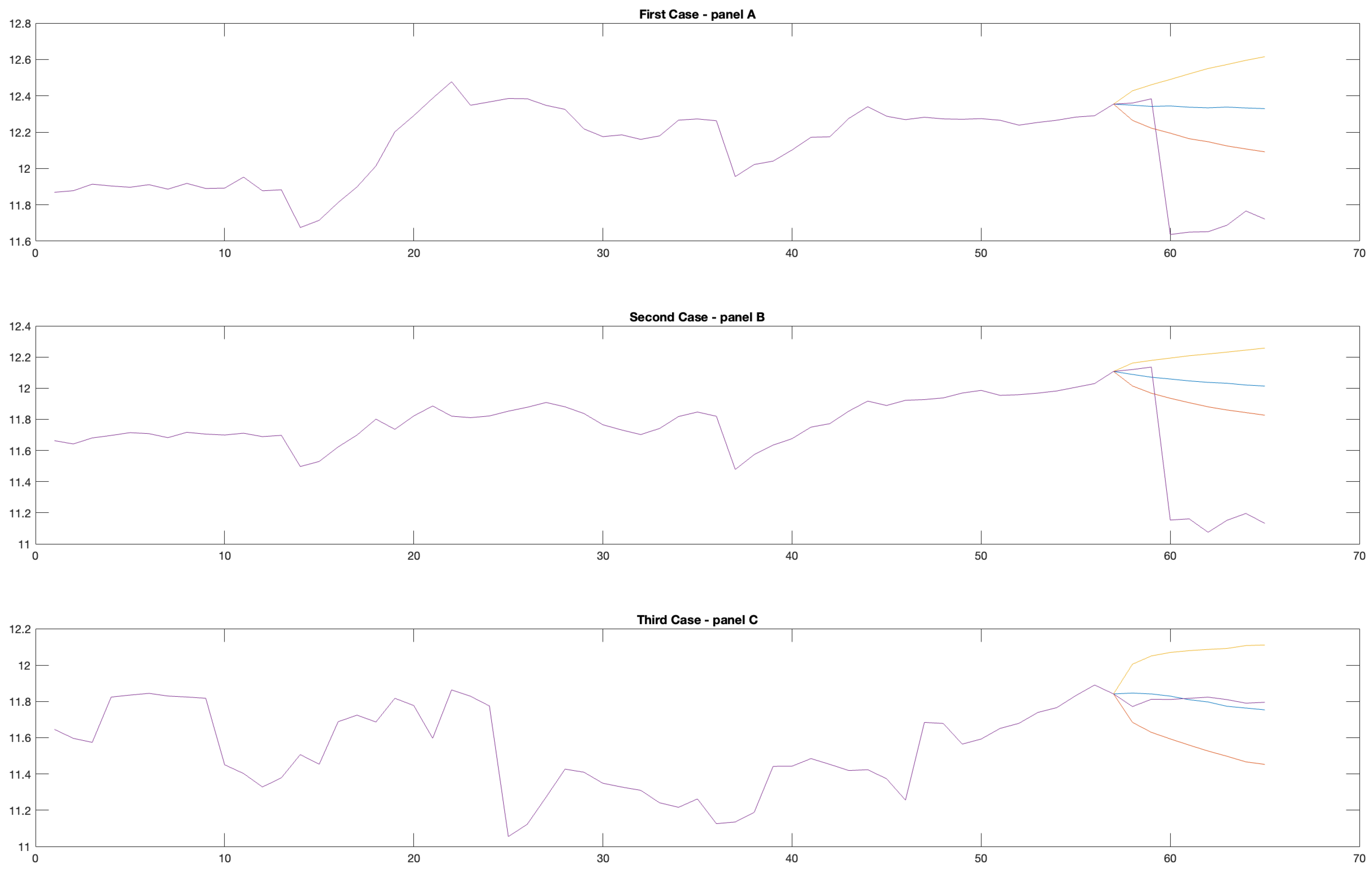
To complete the analysis, three density forecasts on the outcome of interest were performed (Figure 1). The first case (panel A) evaluated only the macroeconomic financial indicators, the second forecast (panel B) accounted for socioeconomic and healthcare statistics as well, and the third and final case (panel C) was run on all subsets of predictors, including demographic and environment indicators and exogenous factors on the regional disparity and characteristics.

The density forecasts were performed by running 100,000 iterations per each random start, spanning the period from 1990 to 2022. The h steps ahead forecast period refers to the years 2023 and 2024 ($h=2$) for replicating the productivity dynamics in the current year and studying them in the next future year (2024). The associated computational costs were minimized, ensuring consistent posterior estimates and dimension reduction.5 The yellow and red lines denote the 95% confidence bands, and the blue and purple lines denote the conditional and unconditional projections of the outcomes of interest for each time period $T+h$, respectively.

According to Figure 1, the forecasts in panel A matter more than the other two cases (panels B and C). This was an expected result when predicting the productivity growth while assuming an unexpected shock in the real and financial dimensions. Indeed, the density forecasts were higher, displaying larger productivity growth over time. In addition, when focusing on the conditional forecasts for the years 2023 and 2024 (blue line), the productivity tended to maintain a trend similar to the previous years. However, when focusing on the unconditional projections (purple line), they strongly diverged because of the presence of endogeneity issues and misspecified dynamics.

In the second case (panel B), where socioeconomic and healthcare factors were also accounted for, the productivity dynamics changed. The density forecasts showed lower magnitudes over time, and the conditional prediction for the years 2023 and 2024 displayed a slightly pronounced decrease, reaching levels lower than the previous years (before the 2020 pandemic). Moreover, the confidence interval containing the conditional forecasting (yellow and red lines) were smaller and tighter than those in panel A. However, in this case, the unconditional projections also totally diverged, even at lower magnitudes. This suggests that the endogeneity and misspecification problems matter again.

Then, the third case included geographical and regional characteristics (panel C). In this specific case, four important results were achieved. First, the productivity dynamics showed strong seasonal components, mainly in accordance with some triggering events such as the 2008 Great Recession, post-crisis recovery programs, and the 2020 pandemic. Second, the upper and lower bound confidence intervals included either conditional or unconditional projections, minimizing the effects of potential endogeneity issues and misspecified dynamics. Third, the same confidence interval tended to be much larger and thicker than the ones observed in panels A and B because of significant cross-region heterogeneity. Fourth, the density forecasts for the years 2023 and 2024 were lower and showed a persistent decrease in the coming years (at least when focusing on the short- and medium-term periods).

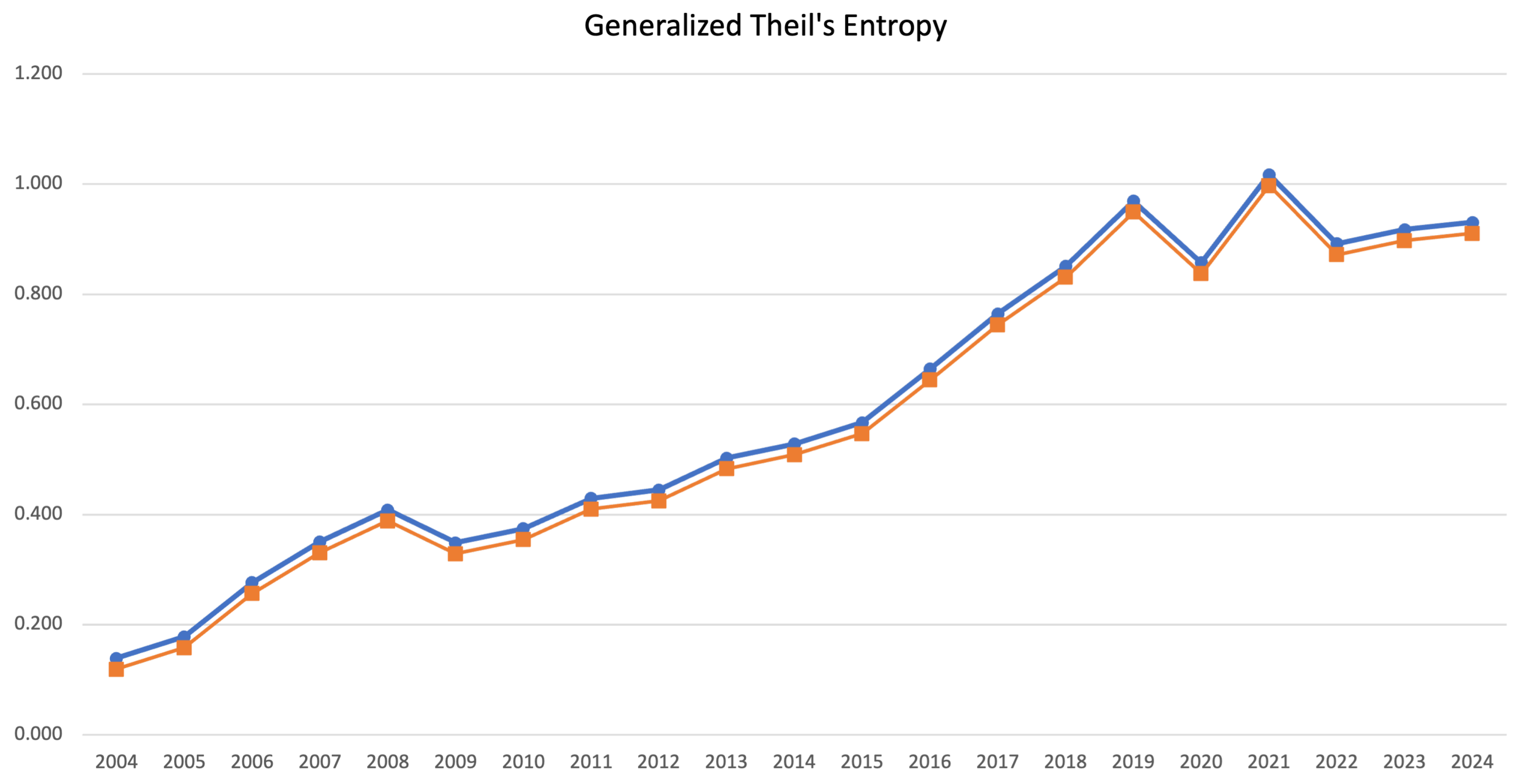
To better address the question of if it is possible to predict pandemic diseases, the generalized Theil’s entropy index was employed, and it displayed in Figure 2. It was computed by drawing the outcomes of interest for every region, weighted by the proportion of the population with respect to the total (blue line) and their conditional projections (red line), obtained through the forward recursions in Equation (19). The time period used ran from 2004 to 2024. The conditional projections were quite close to the observed weighted outcomes, highlighting the consistency and accuracy of the WLB algorithm in fitting the data. Focusing on the year 2019, a sudden fall in productivity was observed until 2020. Then, a totally opposite trend was achieved up to a recorded higher productivity level in 2021. However, in the year 2021, the productivty dynamics changed again by showing not only a significant decrease but also a downward trend with respect to the past. According to these findings, it is unlikely to predict ‘ex ante’ pandemic diseases, but it would be possible to control the contagion and then significantly face their aftereffects on the economy. For instance, when unexpected shocks significantly matter and affect productivity dynamics, more attention should be payed not only to the strictly related macroeconomic financial indicators but also the socioeconomic demographic factors that are similarly relevant nowadays.

During the 2020 pandemic, the global outbreak of public health emergencies merely focused on the health sector and disease-related costs. However, a more partial and comprehensive approach would be essential to evaluate the overall economic development impacts of the global pandemic. Indeed, widespread disease has led to economy-wide shocks to both the supply and consumption sides. In addition, the consistent decrease in consumption also negatively affected the global economy, which in turn caused spillover effects for China’s regional economy through globalized international trade. Relevant government departments should have payed more attention to structural reforms not only for improving the public health system but also building a high-quality mode of economic growth and restructuring global value chains. All these features were present during the 2020 pandemic and still are today but without appropriate diversification purposes dealing with the compelling need of a country or specific region. Maybe, according to the productivity dynamics in Figure 2, a contagion lasting more than 2 years would have been addressed better through more specific and substantial measures and with lower development times.

From a global perspective, the 2020 pandemic has highlighted the need to jointly address health issues with the well-being and lives of citizens, prosperity and stability of societies and economies, and sustainable development. Health challenges are quickly evolving and rapidly changing the geopolitical environment due to the impact of three additional planetary crises: climate change, biodiversity, and pollution. At the same time, new opportunities linked to areas like research or digitalization have arisen. Thus, a global health strategy is needed to provide a new coherent, effective, and focused policy worldwide. The Global Gateway6 represents the close strategy of the European Health Union, which protects the well-being of Europeans and the resilience of their health systems. The main aim of this strategy is that the European Union (EU) should deepen its interest in higher attainable standards of health based on fundamentally specific values such as solidarity, equity, and respect for human rights. Infectious diseases represent a heavy burden on many countries, and high infant and maternal mortality rates are matters to be accounted for. This highlights the need to address global health security programs to better prevent and be more resilient to future pandemics. The first two essential EU priorities are investing in the well-being of people and reaching universal health coverage with much stronger health systems. However, these priorities are rather different from 2010, and other related important drivers of ill health should be addressed in an integrated manner, such as climate change, environmental degradation, and humanitarian crises aggravated by the recent and current Russia-Ukraine war. Thus, it is essential to define a wide number of policies focusing on a global health agenda. Overall, global governance should require a new specific focus to keep strong and constant collaboration with the World Health Organization. Further cooperation should be built through the G7, G20, and other global and regional partners. The EU’s policies should ensure coherent actions with them to avoid the existing gaps in global governance. To support these strategies’ objectives, extremely strong cooperation with the private sector, civil society, and other stakeholders is needed.

Sensitivity Analysis and Heterogeneity Issues

In the current subsection, a counterfactual assessment is addressed to check the sensitivity and robustness analysis, and dynamic panel data with the generalized method of moments (DPDP-GMM) are assessed to investigate endogeneity issues in depth.

Concerning the former, the WLB procedure was performed by using a reduced time series on the same sample of 277 regions for 23 countries and 98 endogenous predictors over the period of 2000–2022. This time period was chosen for two reasons: a sufficiently large number of observations was still ensured ($T=23$), and the last two main global crises (the 2008 financial crisis and the 2020 pandemic) followed to be dealt with. Moreover, different priors were defined for the hyperparameters, allowing for different bounds. In Equation (23), ${\vartheta }_0$ and ${\rho }_0$ were set to $0.90$ and $0.1$, respectively. In Equation (24), ${\alpha }_0$ and ${\nu }_0$ were set to $1.0$ and $0.1$, respectively. Thus, the posterior $\widehat{\rho }={\rho }_0·\overline{\nu }\cong 0.10·(0.10·\overline{\kappa })$ would be equal to $0.009$ in the case of constant volatility and $0.016$ in the case of volatility changes. In both cases, the posterior $\widehat{\rho }$ would approximately converge at the same value. The posterior $\widehat{\vartheta }$ will be always close to zero if the volatilities matter and slightly larger otherwise (≅0.10). Finally, the posterior $\overline{\alpha }={\alpha }_0·\kappa$ will assume larger values, corresponding exactly to the decay factor in the case of volatility (≅1.0) and no time shift (≅0.90). According to these model specifications, the final subset of predictors is unchanged with the variable selection focusing on ‘inclusion’ probabilities (PMPs). Moreover, the CPSs tend to decrease for the most predictors because of not properly disentangling volatilty from coefficient changes when computing $\widehat{\rho }$, the relevant scale parameter for ${\sigma }^2$. However, by construction, the WLB procedure would always ensure sufficient accuracy. Indeed, when letting volatility changes be treated as permanent shifts in the case of dynamically changing variables, an unexpected shock would be absorbed in a certain $M_l$ during the shrinking procedure and then included in the final submodel solution. The estimation results are displayed in

Table 2. Counterfactual assessment: sensitivity analysis.

Idx.	Predictor	Unit	CPS
Macroeconomic Financial Indicators
1	unit labor cost	% values	$0.947$
2	consumer price index	% GDP	$0.011$
3	financial transactions	% GDP	$0.951$
4	employment by age (15–64)	% Tot. Pop.	$0.966$
5	labor force, age 15–64	logarithm	$0.839$
6	unemployment rate by age (15–74)	% Tot. Pop.	$0.009$
7	risk of poverty by age (15–74)	% Tot. Pop.	$0.033$
8	weighted income per capita	% logarithm	$0.947$
9	wage and salaried workers	% Tot. Emp.	$0.928$
10	gross fixed capital formation	% GDP	$0.911$
Socioeconomic and Healthcare Factors
11	overweight	std. rates per 100 people	$0.026$
12	consumption of tobacco	% adults (15+)	$0.013$
13	consumption of alcohol	std. rates per 100 people	$0.021$
14	current health expenditure	% GDP	$0.934$
15	$R\&D$ expenditure	% GDP	$0.917$
16	fertility rate	% Tot. Pop.	$0.885$
17	capital health expenditure	% GDP	$0.893$
18	death rate	per 1000 people	$0.027$
19	secondary school enrollment	% Tot. Pop.	$0.884$
20	social participation	% Tot. Pop.	$0.817$
21	tertiary educational attainment	% Tot. Pop. (25–64)	$0.934$
22	household price index	% GDP	$0.881$
Demographic and Environment Factors
23	rural population	% Tot. Pop.	$0.794$
24	urban population	% Tot. Pop.	$0.814$
25	population growth	% Tot. Pop.	$0.962$
26	total population	logarithm	$0.857$
27	energy use	% GDP	$0.791$
28	total CO2 emission	% Tot. Pop.	$0.028$
29	human capital	logarithm	$0.815$
30	internet use	% GDP	$0.776$
Region–Specific Characteristics
-	$d_{1t}$	1 = northwestern, northeastern Europe; 0 = southwestern, southeastern Europe
-	$d_{2t}$	1 = developed; 0 = developing
-	$d_{3t}$	1 = high economic status; 0 = low economic status
-	Real Growth Rate of GDP	Percentage Change

The Table is split as follows: the first column denotes the predictor number; the second column displays the predictors; the third column refers to the measurement unit; and the last column displays the CPSs. The last row refers to the outcome of interest. The contraction Tot. Pop. stands for ‘total population’, and Tot. Emp. stands for ‘total employed people’. All data refer to Eurostat database.

.

Regarding endogeneity issues and further sensitivity analysis, four DPD-GMM models were evaluated according to the the estimation outputs in Table 1.7 Model 1 includes all the predictors with CPSs strictly close to one or zero over the time period of 1990–2022 (full panel set). Model 2 includes the same previous number of predictors but over the subsample of 2000–2022 (reduced panel set). Model 3 refers to the only the predictors with CPSs strictly close to one or zero dealing with only two groups (socioeconomic healthcare and demographic environment factors) over the time period of 1990–2022 (full panel subset). Model 4 refers to the same previous number of predictors over the subsample of 2000–2022 (reduced panel subset). Here, some considerations are in order. (1) When addressing endogeneity issues (i.e., the error terms are serially correlated with potential covariates violating one of the assumptions of regression models (independent and identically distributed error terms)), dynamic panel data is a useful approach for modeling unobserved heterogeneity by using correct instruments for the endogenous variables from lower to higher orders (Arellano and Bond 1991; Blundell and Bond 1998). (2) In dynamic panel models, when series show strong linear dependencies and dominance of cross-sectional variability (just as in this case), a GMM system is an efficient method for modeling these instruments for effective treatment of endogeneity biases concerning the variables in the estimation. (3) Heteroskedasticity problems are dealt with using robust standard errors across all estimations. (4) Stationarity is checked using a Fisher-type test (Choi 2001), performing well for unbalanced panel datasets (just as in this case) and assuming independently distributed normal error terms for all units (i) and time (t).

In

Table 3. Diagnostic test in dynamic panel regressions with GMM system.

Test Statistic	Model 1	Model 2	Model 3	Model 4
Robustness
$Q_S$ (p-values)	$236.04\left(0.00\right)$	$217.03\left(0.00\right)$	$102.01\left(0.03\right)$	$97.28\left(0.04\right)$
$Q_{AB}$ (p-values)	$2.95\left(0.40\right)$	$2.73\left(0.32\right)$	$1.87\left(0.07\right)$	$1.66\left(0.09\right)$
Observations
Year dummies	Yes	Yes	Yes	Yes
Region dummies	Yes	Yes	No	No
Regions	277	277	277	277
Time series (T)	33	23	33	23

The table addresses two main test statistics with related p values (in parentheses) to check validity of the instruments and efficiency of the estimates in the dynamic panel regressions. They are Sargan’s test for over-identification ($Q_S$) and the Arellano–Bond serial correlation test ($Q_A$). Information on the data is also displayed.

, two main diagnostic tests to check the validity of the instruments and efficiency of the estimates in the DPD-GMM models are displayed: Sargan’s test for over-identification ($Q_S$), highlighting the performance and usefulness of the dynamic panel in dealing with endogenity issues and functional forms of misspecification, and the Arellano–Bond test ($Q_{AB}$) for the first- and second- order serial correlation of residuals (Arellano and Bond 1991). Two main findings can be addressed. First, the results in Models 1 and 2 were quite close, highlighting the performance of the WLB procedure in selecting the promising subset of predictors to be estimated and the usefulness of DPD-GMM models for use in potential econometric approaches. Second, when considering a constrained panel set, endogeneity biases and serial correlations were not efficiently minimized because of omitting potential non-health-related indicators and region-specific characteristics when studying pandemic diseases and their effects on economic development. These results are in line with the density forecasts performed in Figure 1.

5. Concluding Remarks

This study improves the existing literature on predicting pandemic diseases and their effects on economic development across a large set of European and non-European regions. A penalized Bayesian approach-based variable selection procedure is involved to reduce the dimensionality of the model and parameter space and thus select a promising subset of predictors affecting the outcomes of interest.

An empirical example on 277 regions for 23 countries described the estimating procedure and forecasting performance, covering the period of 1990–2022. The forecast horizon referred to the years 2023 and 2024 in order to replicate the productivity dynamics in the current year and study them in the future.

According to the estimation results, conditional and unconditional density forecasts on the productivity dynamics were conducted to highlight how the promising subset of covariates would help predict potential pandemic diseases. Here, three different cases were addressed, accounting for different subsets of predictors. The aim was to highlight how the presence of endogeneity issues and model misspecification affected the estimates when dealing with time-varying parameters and high dimensionality.

From a policy perspective, the global outbreak of public health emergencies has merely focused on the health sector and disease-related costs. Thus, relevant government departments should have paid more attention to structural reforms not only for improving the public health system but also building a high-quality mode of economic growth and restructuring the global value chains. In this way, through prudent long-term policies and more specific and substantial measures, the contagion would have been better addressed with lower development times and higher efficiency in terms of market opportunities, innovation, and consumption features.

The empirical results reported herein should be considered in light of some limitations. Firstly, even if the variables were time-varying, potential volatility changes were treated as permanent shifts and then replaced by coefficient changes. Future improvements might consider, for example, time-varying log volatilities and model them through MCMC implementations (e.g., Metropolis–Hastings and expectation–maximization algorithms). Then, an in-depth analysis might reveal the existence of further regional patterns, evaluated by involving in the variable selection procedure hierarchical fuzzy Bayesian clustering algorithms. Finally, this study did not investigate the causal relationship between the outcome of interest and the subset of predictors, which was beyond the scope of this paper. Related works might consider and discuss in depth the direct and indirect causal links between them.

References

- Abrhám, James, and Milan Vošta. 2022. Impact of the COVID-19 pandemic on eu convergence. Journal of Risk and Financial Management 15: 384. [Google Scholar] [CrossRef]
- Adamek, Robert, Stephan Smeekes, and Ines Wilms. 2023. Lasso inference for high-dimensional time series. Journal of Econometrics 235: 1114–43. [Google Scholar] [CrossRef]
- Arellano, Manuel, and Stephen Bond. 1991. Some tests of specification for panel data: Monte carlo evidence and an application to employment equations. The Review of Economic Studies 58: 277–97. [Google Scholar] [CrossRef]
- Blundell, Richard, and Stephen Bond. 1998. Initial conditions and moment restrictions in dynamic panel data models. Journal of Econometrics 87: 115–43. [Google Scholar] [CrossRef]
- Breiman, Leo, and Philip Spector. 1992. Submodel selection and evaluation in regression. the x-random case. International Statistical Review 60: 291–319. [Google Scholar] [CrossRef]
- Choi, In. 2001. Unit root tests for panel data. Journal of International Money and Finance 20: 249–72. [Google Scholar] [CrossRef]
- Fan, Jianqing, and Runze Li. 2001. Variable selection via nonconcave penalized likelihood and its oracle properties. Journal of the American Statistical Association 96: 1348–60. [Google Scholar] [CrossRef]
- Gelfand, Alan E., and Dipak K. Dey. 1994. Bayesian model choice: Asymptotics and exact calculations. Journal of the Royal Statistical Society: Series B 56: 501–14. [Google Scholar]
- Gungoraydinoglu, Ali, Ilke Öztekin, and Özde Öztekin. 2021. The impact of COVID-19 and its policy responses on local economy and health conditions. Journal of Risk and Financial Management 14: 233. [Google Scholar] [CrossRef]
- Ismail, Shah, Hina Naz, Sajid Ali, Amani Almohaimeed, and Showkat A. Lone. 2023. A new quantile-based approach for lasso estimation. Mathematics 11: 1452. [Google Scholar] [CrossRef]
- Jang, Dae-Heung, and Christine M. Anderson-Cook. 2016. Influence plots for lasso. Journal of Risk and Financial Management 33: 1317–26. [Google Scholar] [CrossRef]
- Kass, Robert E., and Adrian E. Raftery. 1995. Bayes factors. Journal of American Statistical Association 90: 773–95. [Google Scholar] [CrossRef]
- Lu, Wenbin, Yair Goldberg, and J. P. Fine. 2012. On the robustness of the adaptive lasso to model misspecification. Biometrika 99: 717–31. [Google Scholar] [CrossRef]
- Madigan, David, and Adrian E. Raftery. 1994. Model selection and accounting for model uncertainty in graphical models using occam’s window. Journal of American Statistical Association 89: 1535–46. [Google Scholar] [CrossRef]
- Madigan, David, Jeremy York, and Denis Allard. 1995. Bayesian graphical models for discrete data. International Statistical Review 63: 215–32. [Google Scholar] [CrossRef]
- Masini, Ricardo P., Marcelo C. Medeiros, and Eduardo F. Mendes. 2022. Regularized estimation of high-dimensional vector autoregressions with weakly dependent innovations. Journal of Time Series Analysis 43: 532–57. [Google Scholar] [CrossRef]
- Medeiros, Marcelo C., and Eduardo F. Mendes. 2016. l1-regularization of high-dimensional time-series models with non-gaussian and heteroskedastic errors. Journal of Econometrics 191: 255–71. [Google Scholar] [CrossRef]
- Mohammad, Arashi, Asar Yasin, and Yüzbaşi Bahadır. 2021. Slasso: A scaled lasso for multicollinear situations. Journal of Statistical Computation and Simulation 91: 3170–83. [Google Scholar] [CrossRef]
- Pacifico, Antonio. 2020. Robust open bayesian analysis: Overfitting, model uncertainty, and endogeneity issues in multiple regression models. Econometric Reviews 40: 148–76. [Google Scholar] [CrossRef]
- Pulawska, Karolina. 2021. Financial stability of european insurance companies during the COVID-19 pandemic. Journal of Risk and Financial Management 14: 266. [Google Scholar] [CrossRef]
- Raftery, Adrian E., David Madigan, and Chris T. Volinsky. 1995. Accounting for model uncertainty in survival analysis improves predictive performance. Bayesian Statistics 6: 323–49. [Google Scholar]
- Raftery, Adrian E., David Madigan, and Jennifer A. Hoeting. 1997. Bayesian model averaging for linear regression models. Journal of American Statistical Association 92: 179–91. [Google Scholar] [CrossRef]
- Tibshirani, Robert. 1996. Regression shrinkage and selection via the lasso. Journal of the Royal Statistical Society: Series B 58: 267–88. [Google Scholar] [CrossRef]
- Uematsu, Yoshimasa, and Takashi Yamagata. 2023. Inference in sparsity-induced weak factor models. Journal of Business and Economic Statistics 41: 126–39. [Google Scholar] [CrossRef]
- Vidaurre, Diego, Concha Bielza, and Pedro Larrañaga. 2013. A survey of l1 regression. International Statistical Review 81: 361–87. [Google Scholar] [CrossRef]
- Wenjiang, J. Fu. 1998. Penalized regressions: The bridge versus the lasso. Journal of Computational and Graphical Statistics 7: 397–416. [Google Scholar]
- Wong, Kam C., Zifan Li, and Ambuj Tewari. 2020. Lasso guarantees for beta-mixing heavy-tailed time series. Annals of Statistics 48: 1124–42. [Google Scholar] [CrossRef]
- Wu, Wei B., and Ying N. Wu. 2016. Performance bounds for parameter estimates of high-dimensional linear models with correlated errors. Electronic Journal of Statistics 10: 352–79. [Google Scholar] [CrossRef]
- Yang, Xiaoxing, and Wushao Wen. 2018. Ridge and lasso regression models for cross-version defect prediction. IEEE Transactions on Reliability 67: 885–96. [Google Scholar] [CrossRef]
- Zhang, Cun-Hui, and Stephanie S. Zhang. 2014. Confidence intervals for low dimensional parameters in high dimensional linear models. Journal of the Royal Statistical Society: Series B 76: 217–42. [Google Scholar] [CrossRef]
- Zou, Hui. 2006. The adaptive lasso and its oracle properties. Journal of the American Statistical Association 101: 1418–29. [Google Scholar] [CrossRef]
Figure 1.
The plot for conditional and unconditional projections for the outcome of interest, spanning the period from 1990 to 2022. The forecast horizon refers to the years 2023 and 2024 (). The Y and X axes represent the conditional projections and sampling distribution in years, respectively. Concerning the latter, the reference period is 1990 (0); 1995 (10); 2000 (20); 2005 (30); 2010 (40); 2015 (50); 2022 (60); and 2024 (<70).
Figure 2.
Plot of the generalized Theil’s entropy index from 2004 to 2024. This corresponds to the outcomes of interest weighted by the proportion of the population with respect to the total (blue line) and their conditional projections (red line) obtained through the forward recursions in Equation (19).